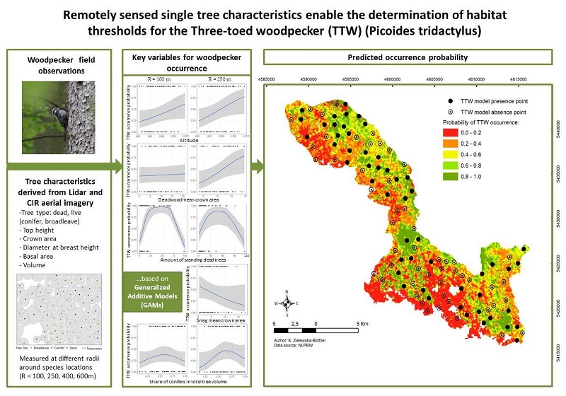
Remotely Sensed Single Tree Data Enable the Determination of Habitat Thresholds for the Three-Toed Woodpecker (Picoides tridactylus)


Abstract
:
1. Introduction
2. Materials and Methods
2.1. Study Area
2.2. Remote Sensing Data
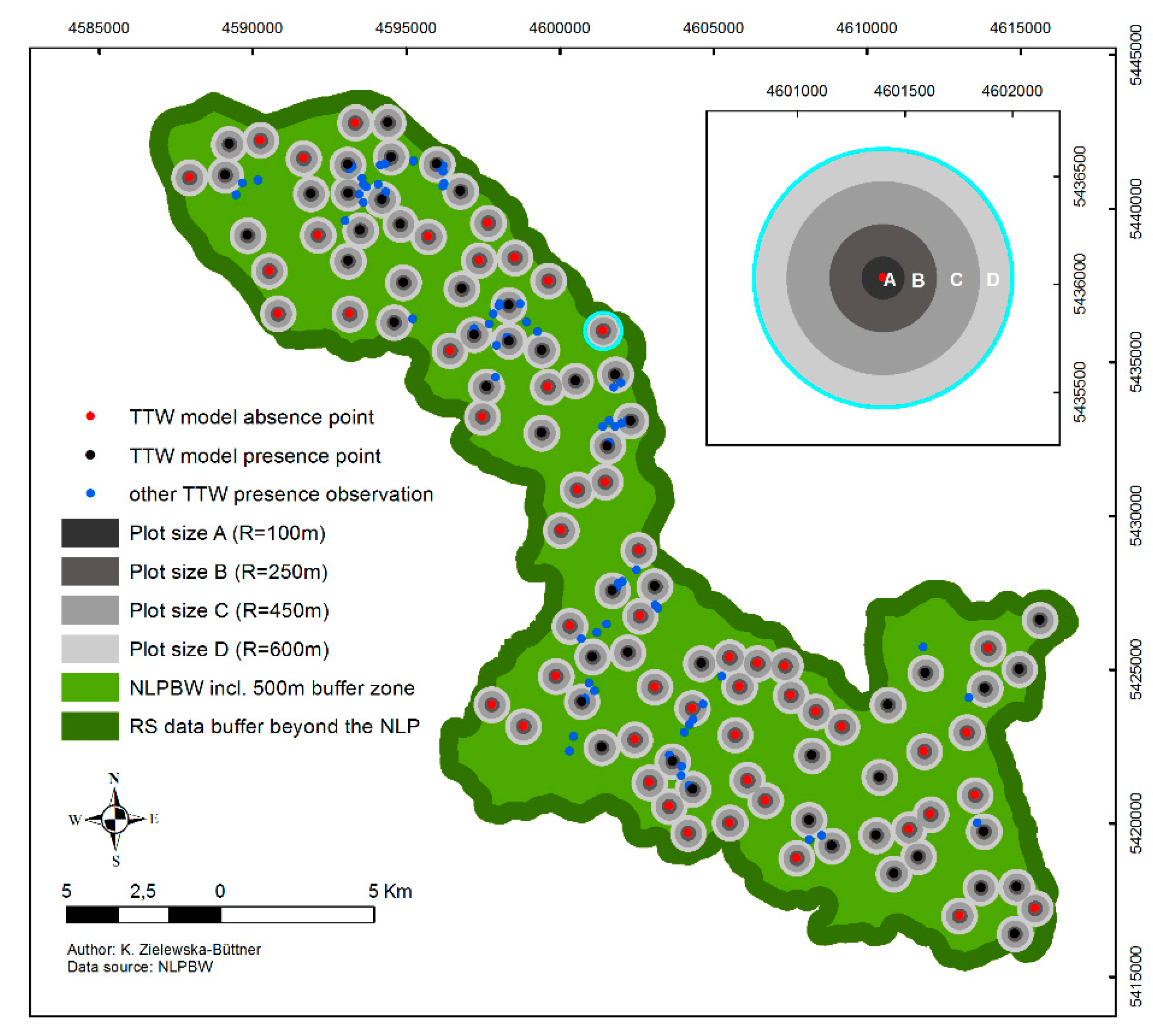
2.3. Species Data and Sampling Design
- R = 100 m to evaluate the habitat characteristics in close vicinity of the TTW presence locations.
- R = 250 m (19.6 ha) representing the minimum reported home range of an individual TTW under excellent habitat conditions (ca. 16–19 ha [85]);
2.4. Predictor Variables
2.5. Statistical Analysis
3. Results
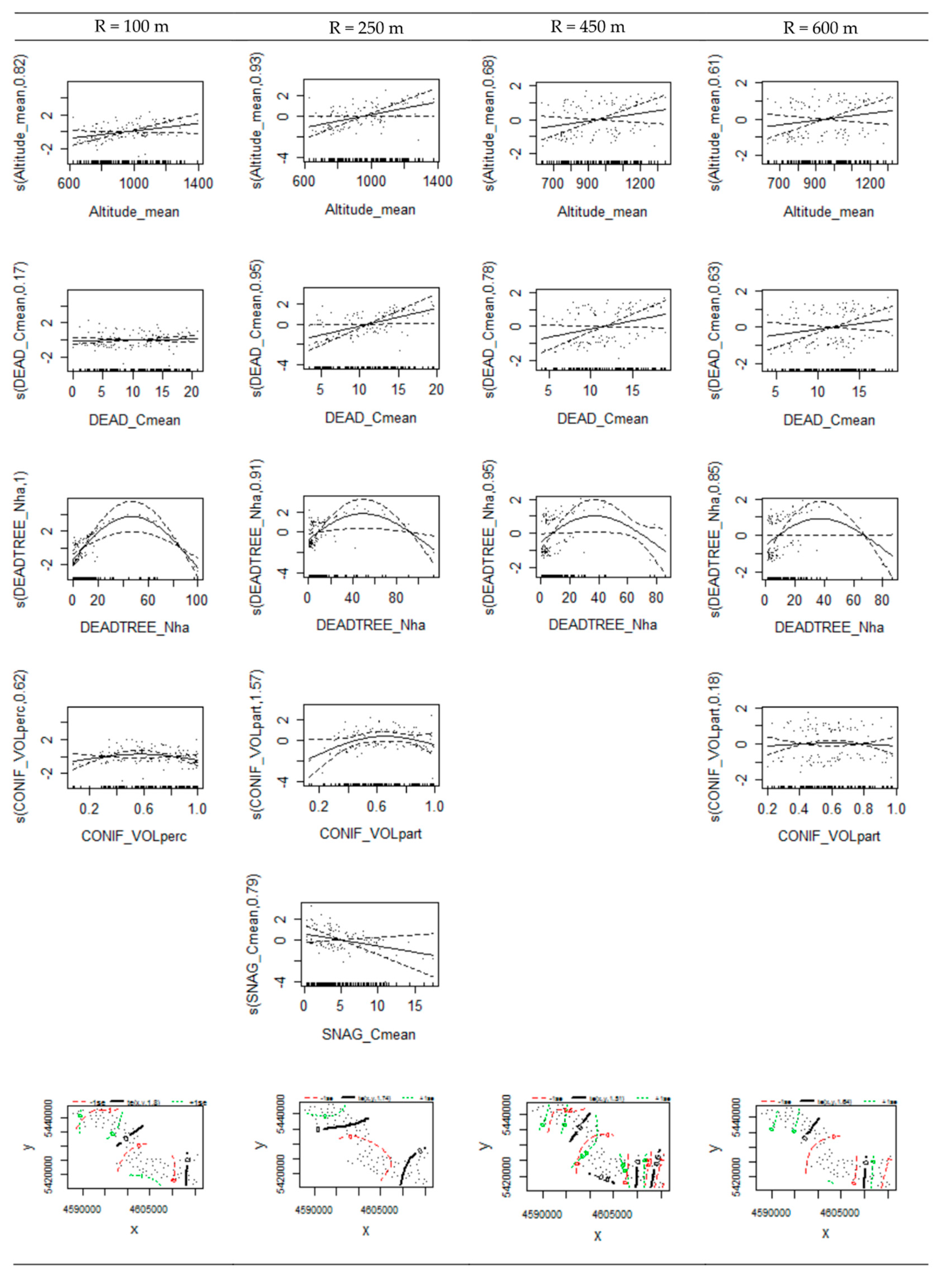
3.1. Habitat Selection
3.2. Model Performance
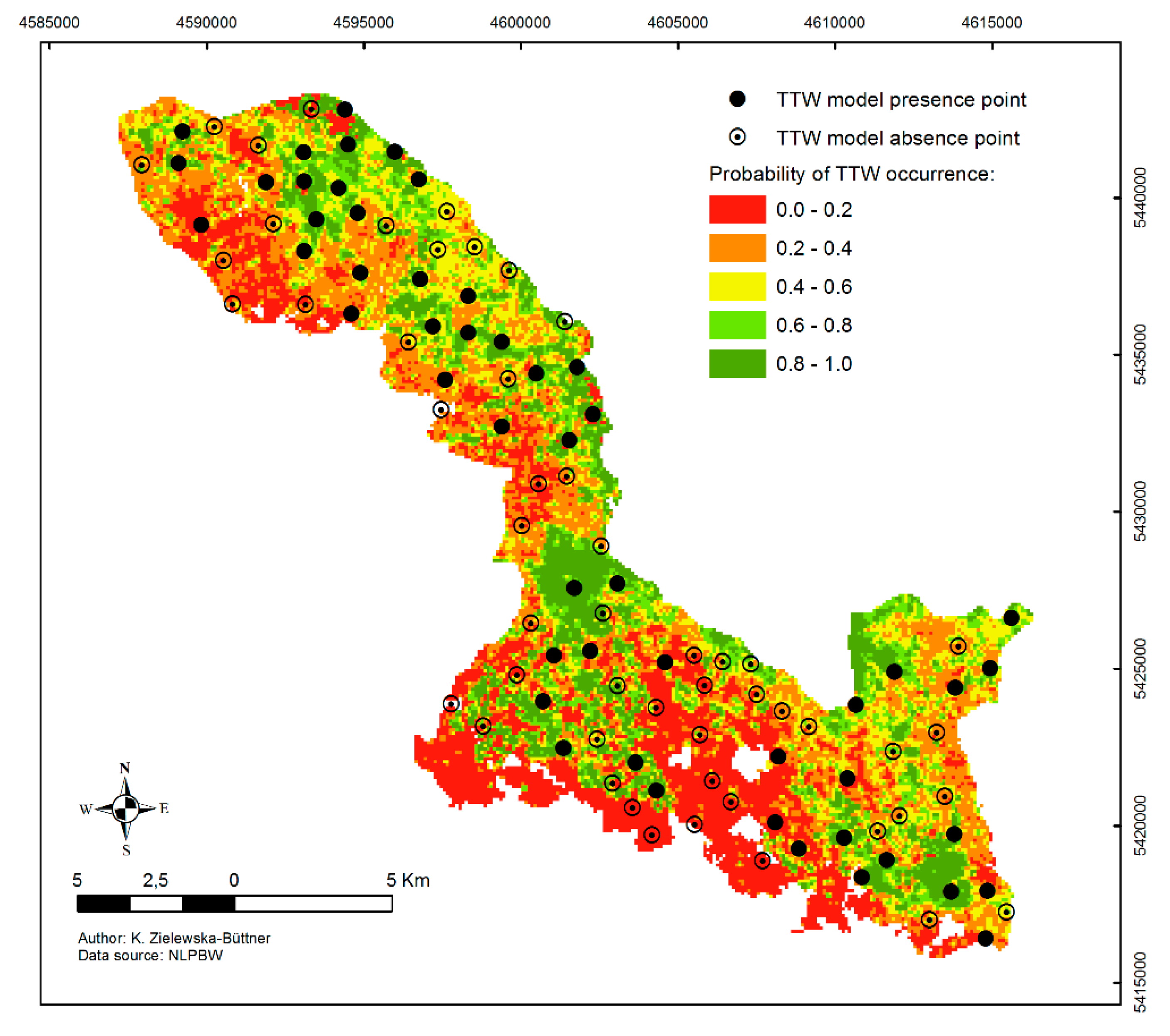
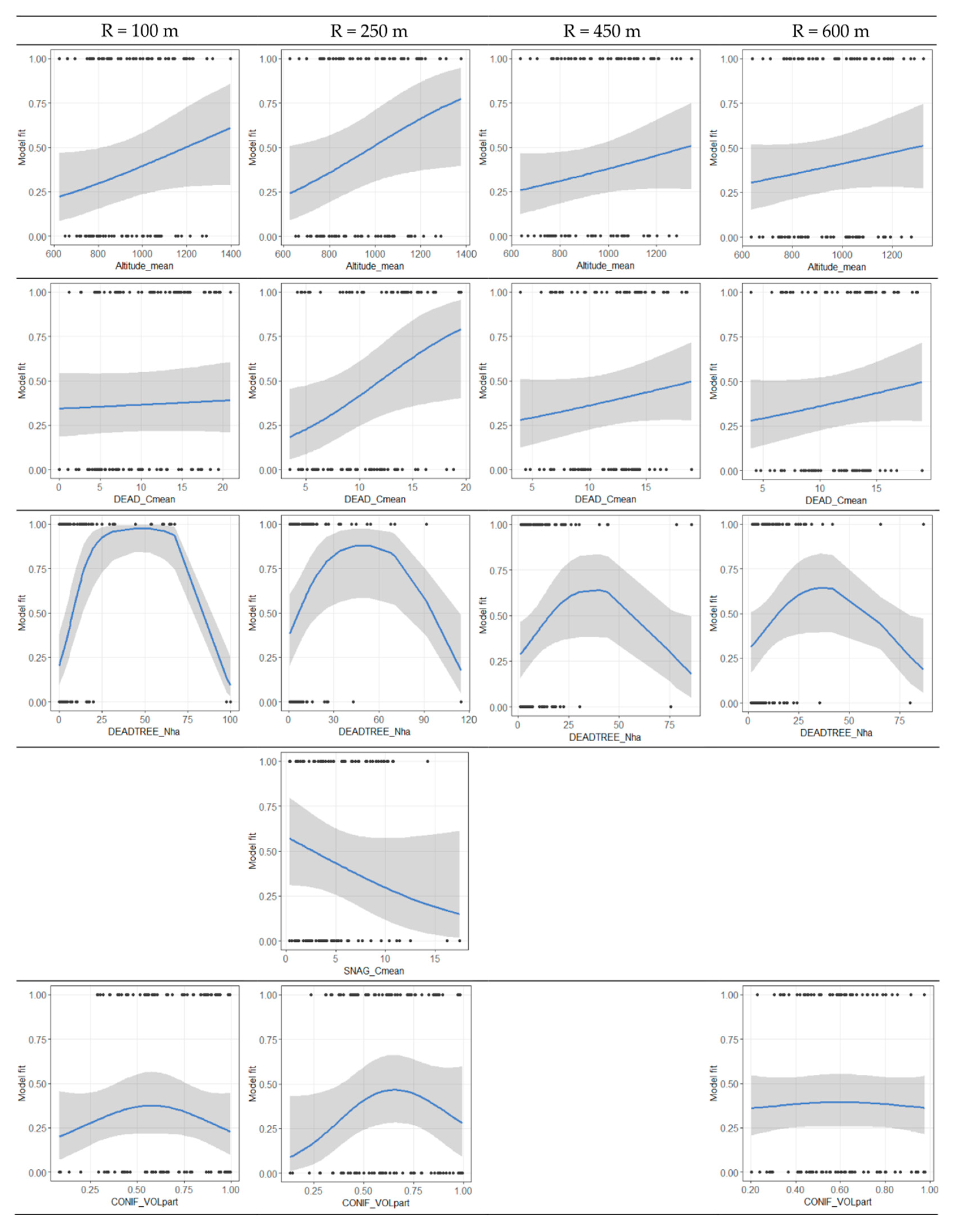
3.3. Model Prediction
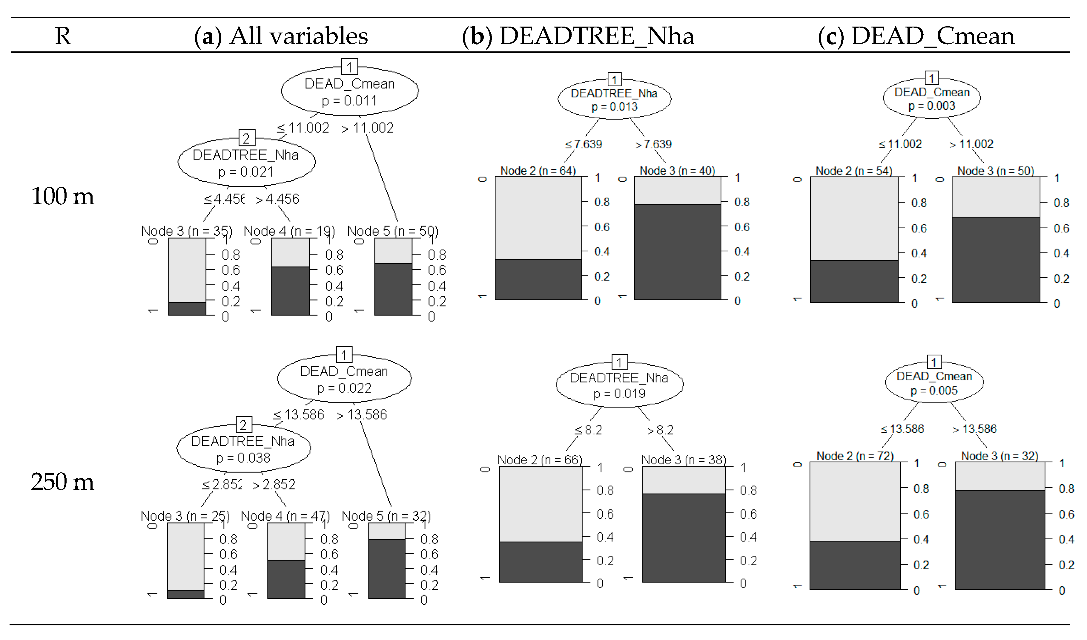
3.4. Variable Thresholds
4. Discussion
4.1. Remote Sensing Data
4.2. Species Data
4.3. Modelling Approach
4.4. TTW Habitat Selection
4.5. Management Recommendations
5. Conclusions
Author Contributions
Funding
Acknowledgments
Conflicts of Interest
Appendix A

| R | Variable | Unit | All Plots | Presence | Absence | |||
|---|---|---|---|---|---|---|---|---|
| Mean | SD | Mean | SD | Mean | SD | |||
| 100 | Altitude_mean | m a.s.l. | 953.84 | 182.37 | 990.93 | 187.98 | 916.74 | 170.36 |
| CONIF_Nha | N/ha | 172.96 | 91.54 | 159.96 | 90.21 | 185.95 | 91.89 | |
| DEAD_Cmean | m2 | 10.35 | 5.32 | 11.92 | 5.13 | 8.78 | 5.09 | |
| DEADTREE_Nha | N/ha | 12.75 | 19.74 | 17.55 | 19.56 | 7.95 | 18.91 | |
| SNAG_Cmean | m2 | 4.76 | 4.28 | 5.19 | 4.01 | 4.34 | 4.53 | |
| LIVE_Nha | N/ha | 299.55 | 134.15 | 276.43 | 137.98 | 322.66 | 127.35 | |
| CONIF_VOL | % | 0.65 | 0.24 | 0.66 | 0.22 | 0.65 | 0.27 | |
| DEADCIR_part | % | 0.04 | 0.09 | 0.05 | 0.09 | 0.03 | 0.09 | |
| 250 | Altitude_mean | m a.s.l. | 953.53 | 180.50 | 989.86 | 184.95 | 917.20 | 170.00 |
| CONIF_Nha | N/ha | 178.28 | 78.48 | 163.82 | 75.10 | 192.73 | 79.84 | |
| DEAD_Cmean | m2 | 11.01 | 4.13 | 12.16 | 4.14 | 9.86 | 3.82 | |
| DEADTREE_Nha | N/ha | 12.58 | 18.97 | 16.94 | 20.03 | 8.21 | 16.93 | |
| SNAG_Cmean | m2 | 5.02 | 3.63 | 5.48 | 3.33 | 4.56 | 3.89 | |
| LIVE_Nha | N/ha | 311.07 | 116.69 | 290.57 | 119.85 | 331.57 | 110.81 | |
| CONIF_VOLpart | % | 0.63 | 0.22 | 0.63 | 0.21 | 0.63 | 0.24 | |
| DEADCIR_part | % | 0.04 | 0.08 | 0.05 | 0.08 | 0.03 | 0.08 | |
| 450 | Altitude_mean | m a.s.l. | 952.71 | 176.60 | 987.99 | 179.23 | 917.44 | 168.31 |
| CONIF_Nha | N/ha | 184.81 | 71.52 | 168.79 | 69.50 | 200.84 | 70.54 | |
| DEAD_Cmean | m131 | 11.52 | 3.61 | 12.31 | 3.76 | 10.73 | 3.30 | |
| DEADTREE_Nha | N/ha | 11.77 | 15.01 | 15.24 | 17.31 | 8.30 | 11.43 | |
| SNAG_Cmean | m2 | 5.56 | 3.44 | 5.87 | 3.12 | 5.25 | 3.74 | |
| LIVE_Nha | N/ha | 329.25 | 108.90 | 309.69 | 113.58 | 348.81 | 101.35 | |
| CONIF_VOLpart | % | 0.60 | 0.19 | 0.59 | 0.18 | 0.61 | 0.21 | |
| DEADCIR_part | % | 0.37 | 0.65 | 0.47 | 0.73 | 0.28 | 0.56 | |
| 600 | Altitude_mean | m a.s.l. | 951.77 | 173.45 | 986.13 | 174.79 | 917.41 | 166.72 |
| CONIF_Nha | N/ha | 187.38 | 70.91 | 172.16 | 67.59 | 202.60 | 71.51 | |
| DEAD_Cmean | m131 | 11.76 | 3.47 | 12.33 | 3.62 | 11.19 | 3.26 | |
| DEADTREE_Nha | N/ha | 11.96 | 14.24 | 14.50 | 15.71 | 9.43 | 12.24 | |
| SNAG_Cmean | m2 | 5.69 | 3.18 | 5.90 | 2.91 | 5.49 | 3.45 | |
| LIVE_Nha | N/ha | 335.78 | 105.28 | 319.20 | 112.90 | 352.35 | 95.29 | |
| CONIF_VOLpart | % | 0.58 | 0.18 | 0.57 | 0.16 | 0.59 | 0.20 | |
| DEADCIR_part | % | 0.04 | 0.06 | 0.04 | 0.06 | 0.03 | 0.06 | |
| R | Model Fit Measures | Fold_1 | Fold_2 | Fold_3 | Fold_4 | Fold_5 | Mean | SD |
|---|---|---|---|---|---|---|---|---|
| 100 | AIC | 91.00 | 93.32 | 91.55 | 87.59 | 83.49 | 89.39 | 3.49 |
| R-sq.(adj.) | 0.31 | 0.28 | 0.35 | 0.37 | 0.40 | 0.34 | 0.04 | |
| AUC | 0.80 | 0.89 | 0.84 | 0.74 | 0.59 | 0.77 | 0.10 | |
| Sensitivity | 0.91 | 0.82 | 0.50 | 0.70 | 0.80 | 0.75 | 0.14 | |
| Specificity | 0.73 | 0.91 | 0.90 | 0.50 | 0.30 | 0.67 | 0.24 | |
| Correct Class. Rate | 0.82 | 0.86 | 0.70 | 0.60 | 0.55 | 0.71 | 0.12 | |
| Cohen’s Kappa | 0.64 | 0.73 | 0.40 | 0.20 | 0.10 | 0.41 | 0.24 | |
| 250 | AIC | 98.43 | 97.17 | 106.73 | 104.61 | 91.30 | 99.65 | 5.52 |
| R-sq.(adj.) | 0.25 | 0.28 | 0.18 | 0.18 | 0.35 | 0.25 | 0.06 | |
| AUC | 0.65 | 0.74 | 0.83 | 0.71 | 0.60 | 0.71 | 0.08 | |
| Sensitivity | 0.55 | 0.64 | 0.70 | 0.70 | 0.70 | 0.66 | 0.06 | |
| Specificity | 0.55 | 0.82 | 0.80 | 0.60 | 0.50 | 0.65 | 0.13 | |
| Correct Class. Rate | 0.55 | 0.73 | 0.75 | 0.65 | 0.60 | 0.65 | 0.08 | |
| Cohen’s Kappa | 0.09 | 0.46 | 0.50 | 0.30 | 0.20 | 0.31 | 0.15 | |
| 450 | AIC | 104.04 | 105.93 | 113.38 | 109.05 | 104.26 | 107.33 | 3.51 |
| R-sq.(adj.) | 0.18 | 0.16 | 0.09 | 0.13 | 0.19 | 0.15 | 0.04 | |
| AUC | 0.55 | 0.63 | 0.76 | 0.70 | 0.51 | 0.63 | 0.09 | |
| Sensitivity | 0.36 | 0.64 | 0.70 | 0.70 | 0.50 | 0.58 | 0.13 | |
| Specificity | 0.55 | 0.55 | 0.80 | 0.40 | 0.30 | 0.52 | 0.17 | |
| Correct Class. Rate | 0.46 | 0.59 | 0.75 | 0.55 | 0.40 | 0.55 | 0.12 | |
| Cohen’s Kappa | −0.09 | 0.18 | 0.50 | 0.10 | −0.20 | 0.10 | 0.24 | |
| 600 | AIC | 106.22 | 109.15 | 113.70 | 113.15 | 108.39 | 110.12 | 2.87 |
| R-sq.(adj.) | 0.17 | 0.12 | 0.09 | 0.09 | 0.15 | 0.12 | 0.03 | |
| AUC | 0.50 | 0.63 | 0.71 | 0.71 | 0.49 | 0.61 | 0.10 | |
| Sensitivity | 0.46 | 0.64 | 0.50 | 0.60 | 0.50 | 0.54 | 0.07 | |
| Specificity | 0.55 | 0.46 | 0.80 | 0.60 | 0.50 | 0.58 | 0.12 | |
| Correct Class. Rate | 0.50 | 0.55 | 0.65 | 0.60 | 0.50 | 0.56 | 0.06 | |
| Cohen’s Kappa | 0.00 | 0.09 | 0.30 | 0.20 | 0.00 | 0.12 | 0.12 |

References
- Stighäll, K.; Roberge, J.-M.; Andersson, K.; Angelstam, P. Usefulness of biophysical proxy data for modelling habitat of an endangered forest species: The white-backed woodpecker Dendrocopos leucotos. Scand. J. For. Res. 2011, 26, 576–585. [Google Scholar] [CrossRef]
- Müller, D.; Schröder, B.; Müller, J. Modelling habitat selection of the cryptic Hazel Grouse Bonasa bonasia in a montane forest. J. Ornithol. 2009, 150, 717–732. [Google Scholar] [CrossRef] [Green Version]
- Guisan, A.; Thuiller, W. Predicting species distribution: Offering more than simple habitat models. Ecol. Lett. 2005, 8, 993–1009. [Google Scholar] [CrossRef]
- Magg, N.; Müller, J.; Heibl, C.; Hackländer, K.; Wölfl, S.; Wölfl, M.; Bufka, L.; Cervený, J.; Heurich, M. Habitat availability is not limiting the distribution of the Bohemian–Bavarian lynx Lynx lynx population. Oryx 2015, 50, 742–752. [Google Scholar] [CrossRef]
- Vogeler, J.C.; Hudak, A.T.; Vierling, L.A.; Evans, J.; Green, P.; Vierling, K.T. Terrain and vegetation structural influences on local avian species richness in two mixed-conifer forests. Remote Sens. Environ. 2014, 147, 13–22. [Google Scholar] [CrossRef]
- Zellweger, F.; Baltensweiler, A.; Ginzler, C.; Roth, T.; Braunisch, V.; Bugmann, H.; Bollmann, K. Environmental predictors of species richness in forest landscapes: Abiotic factors versus vegetation structure. J. Biogeogr. 2016, 43, 1080–1090. [Google Scholar] [CrossRef]
- Lesak, A.A.; Radeloff, V.C.; Hawbaker, T.J.; Pidgeon, A.M.; Gobakken, T.; Contrucci, K. Modeling forest songbird species richness using LiDAR-derived measures of forest structure. Remote Sens. Environ. 2011, 115, 2823–2835. [Google Scholar] [CrossRef]
- Hirzel, A.H.; Le Lay, G. Habitat suitability modelling and niche theory. J. Appl. Ecol. 2008, 45, 1372–1381. [Google Scholar] [CrossRef] [Green Version]
- Jayathunga, S.; Owari, T.; Tsuyuki, S. Analysis of forest structural complexity using airborne LiDAR data and aerial photography in a mixed conifer–broadleaf forest in northern Japan. J. For. Res. 2018, 29, 479–493. [Google Scholar] [CrossRef]
- White, J.C.; Coops, N.C.; Wulder, M.A.; Vastaranta, M.; Hilker, T.; Tompalski, P. Remote Sensing Technologies for Enhancing Forest Inventories: A Review. Can. J. Remote Sens. 2016, 42, 619–641. [Google Scholar] [CrossRef]
- Zellweger, F.; Morsdorf, F.; Purves, R.S.; Braunisch, V.; Bollmann, K. Improved methods for measuring forest landscape structure: LiDAR complements field-based habitat assessment. Biodivers. Conserv. 2013, 23, 289–307. [Google Scholar] [CrossRef]
- Vogeler, J.C.; Cohen, W.B. A review of the role of active remote sensing and data fusion for characterizing forest in wildlife habitat models. Revista de Teledetección 2016, 45, 1–14. [Google Scholar] [CrossRef]
- Lausch, A.; Bannehr, L.; Beckmann, M.; Boehm, C.; Feilhauer, H.; Hacker, J.M.; Heurich, M.; Jung, A.; Klenke, R.; Neumann, C.; et al. Linking Earth Observation and taxonomic, structural and functional biodiversity: Local to ecosystem perspectives. Ecol. Indic. 2016, 70, 317–339. [Google Scholar] [CrossRef]
- Lindberg, E.; Roberge, J.M.; Johansson, T.; Hjältén, J. Can Airborne Laser Scanning (ALS) and Forest Estimates Derived from Satellite Images Be Used to Predict Abundance and Species Richness of Birds and Beetles in Boreal Forest? Remote Sens. 2015, 7, 4233–4252. [Google Scholar] [CrossRef] [Green Version]
- Bütler, R.; Schlaepfer, R. Spruce snag quantification by coupling colour infrared aerial photos and a GIS. For. Ecol. Manag. 2004, 195, 325–339. [Google Scholar] [CrossRef]
- Ahrens, W.; Brockamp, U.; Pisoke, T. Zur Erfassung von Waldstrukturen im Luftbild. Arbeitsanleitung für Waldschutzgebiete Baden-Württemberg. Waldschutzgebiete Baden-Württemberg 2004, 5, 54. [Google Scholar]
- Rechsteiner, C.; Zellweger, Z.; Gerber, A.; Breiner, F.T.; Bollmann, K. Remotely sensed forest habitat structures improve regional species conservation. Remote Sens. Ecol. Conserv. 2017, 3, 247–258. [Google Scholar] [CrossRef]
- Müller, J.; Stadler, J.; Brandl, R. Composition versus physiognomy of vegetation as predictors of bird assemblages: The role of lidar. Remote Sens. Environ. 2010, 114, 490–495. [Google Scholar] [CrossRef]
- Graf, R.F.; Mathys, L.; Bollmann, K. Habitat assessment for forest dwelling species using LiDAR remote sensing: Capercaillie in the Alps. For. Ecol. Manag. 2009, 257, 160–167. [Google Scholar] [CrossRef]
- Martinuzzi, S.; Vierling, L.A.; Gould, W.A.; Falkowski, M.J.; Evans, J.S.; Hudak, A.T.; Vierling, K.T. Mapping snags and understory shrubs for a LiDAR-based assessment of wildlife habitat suitability. Remote Sens. Environ. 2009, 113, 2533–2546. [Google Scholar] [CrossRef]
- Braunisch, V.; Coppes, J.; Arlettaz, R.; Suchant, R.; Zellweger, F.; Bollmann, K. Temperate mountain forest biodiversity under climate change: Compensating negative effects by increasing structural complexity. PLoS ONE 2014, 9, e97718. [Google Scholar] [CrossRef] [PubMed]
- Froidevaux, J.S.P.; Zellweger, F.; Bollmann, K.; Jones, G.; Obrist, M.K. From field surveys to LiDAR: Shining a light on how bats respond to forest structure. Remote Sens. Environ. 2016, 175, 242–250. [Google Scholar] [CrossRef] [Green Version]
- Kortmann, M.; Hurst, J.; Brinkmann, R.; Heurich, M.; Silveyra González, R.; Müller, J.; Thorn, S. Beauty and the beast: How a bat utilizes forests shaped by outbreaks of an insect pest. Anim. Conserv. 2018, 21, 21–30. [Google Scholar] [CrossRef]
- Säynäjoki, R.; Packalén, P.; Maltamo, M.; Vehmas, M.; Eerikäinen, K. Detection of Aspens Using High Resolution Aerial Laser Scanning Data and Digital Aerial Images. Sensors 2008, 8, 5037–5054. [Google Scholar] [CrossRef] [PubMed] [Green Version]
- Persson, Å.; Holmgren, J.; Söderman, U.; Olsson, H. Tree species classification of individual trees in Sweden by combining high resolution laser data with high resolution near-infrared digital images. Int. Arch. Photogramm. Remote Sens. Spat. Inf. Sci. 2004, 36, 204–207. [Google Scholar]
- Amiri, N.; Polewski, P.; Yao, W.; Heurich, M.; Krzystek, P.; Skidmore, A.K. Feature relevance assessment for single tree species classification using ALS point clouds and aerial imagery. In Proceedings of the Young Professionals Conference on Remote Sensing, Oberpfaffenhofen, Germany, 20–21 October 2016; p. 4. [Google Scholar]
- Dalponte, M.; Bruzzone, L.; Gianelle, D. Fusion of Hyperspectral and LIDAR Remote Sensing Data for Classification of Complex Forest Areas. IEEE Trans. Geosci. Remote Sens. 2008, 46, 1416–1427. [Google Scholar] [CrossRef] [Green Version]
- Heinzel, J.; Koch, B. Investigating multiple data sources for tree species classification in temperate forest and use for single tree delineation. Int. J. Appl. Earth Obs. Geoinf. 2012, 18, 101–110. [Google Scholar] [CrossRef]
- Heinzel, J.; Weinacker, H.; Koch, B. Full automatic detection of tree species based on delineated single tree crowns—A data fusion approach for airborne laser scanning data and aerial photographs. In Proceedings of the SilviLaser 2008, Edinburgh, UK, 17–19 September 2008; p. 10. [Google Scholar]
- Polewski, P.; Yao, W.; Heurich, M.; Krzystek, P.; Stilla, U. Detection of single standing dead trees from aerial color infrared imagery by segmentation with shape and intensity priors. In Proceedings of the 2015 PIA15+HRIGI15—Joint ISPRS Conference 2015, Munich, Germany, 25–27 March 2015; 2015; Volume II-3/W4, pp. 181–188. [Google Scholar]
- Polewski, P.; Yao, W.; Heurich, M.; Krzystek, P.; Stilla, U. Combining Active and Semisupervised Learning of Remote Sensing Data Within a Renyi Entropy Regularization Framework. IEEE J. Sel. Top. Appl. Earth Obs. Remote Sens. 2015, 9, 2910–2922. [Google Scholar] [CrossRef]
- Latifi, H.; Heurich, M.; Hartig, F.; Müller, J.; Krzystek, P.; Jehl, H.; Dech, S. Estimating over- and understorey canopy density of temperate mixed stands by airborne LiDAR data. For. Int. J. For. Res. 2016, 89, 69–81. [Google Scholar] [CrossRef]
- BirdLife, International. European Red List of Birds; Office for Official Publications of the European Communities: Luxembourg, 2016. [Google Scholar]
- Głowaciński, Z.; Makomaska-Juchiewicz, M.; Połczyńska-Konior, G. Red List of Threatened Animals in Poland; Polish Academy of Sciences, Institude of Nature Conservation: Cracow, Poland, 2002. [Google Scholar]
- Bauer, H.-G.; Boschert, M.; Förschler, M.I.; Hölzinger, J.; Kramer, M.; Ulrich, M. Rote Liste und kommentiertes Verzeichnis der Brutvogelarten Baden-Württembergs. 6. Fassung. Stand: 31.12.2013. Naturschutz-Praxis Artenschutz 11; LUBW Landesanstalt für Umwelt, Messungen und Naturschutz Baden-Württemberg: Karlsruhe, Germany, 2016. [Google Scholar]
- Hölzinger, J.; Mahler, U. Die Vögel Baden-Württembergs. Bd. 2 Nicht-Singvögel. 3 Pteroclididae (Flughühner)—Picidae (Spechte); Ulmer: Stuttgart, Germany, 2001; p. 547. [Google Scholar]
- Südbeck, P.; Bauer, H.-G.; Boschert, M.; Boye, P.; Knief, W. The Red List of breeding birds of Germany. Ber. Vogelschutz. 2007, 44, 23–81. [Google Scholar]
- Mikusiński, G.; Gromadzki, M.; Chylarecki, P. Woodpeckers as Indicators of Forest Bird Diversity. Conserv. Biol. 2001, 15, 208–217. [Google Scholar] [CrossRef]
- Thompson, I.D.; Angelstam, P. Special species. In Maintaining Biodiversity in Forest Ecosystems; Hunter, M.L., Ed.; Cambridge University Press: Cambridge, UK, 1999; pp. 434–459. [Google Scholar]
- Bütler, R.; Angelstam, P.; Ekelund, P.; Schlaepfer, R. Dead wood threshold values for the three-toed woodpecker presence in boreal and sub-Alpine forest. Biol. Conserv. 2004, 119, 305–318. [Google Scholar] [CrossRef]
- Saari, L.; Mikusinski, G. Population fluctuations of woodpecker species on the Baltic island of Aasla, SW Finland. Ornis Fenn. 1996, 73, 168–178. [Google Scholar]
- Virkkala, R. Why study woodpeckers? The significance of woodpeckers in forest ecosystems. Ann. Zool. Fenn. 2006, 43, 82–85. [Google Scholar]
- Fayt, P. Population Ecology of the Three-Toed Woodpecker under Varying Food Supplies; University of Joensuu: Joensuu, Finland, 2003. [Google Scholar]
- Pechacek, P.; Krištín, A. Comparative diets of adult and young Threetoed Woodpeckers in a European alpine forest community. J. Wildl. Manag. 2004, 68, 683–693. [Google Scholar] [CrossRef]
- Angelstam, P.; Bütler, R.; Lazdinis, M.; Mikusinski, G.; Roberge, J.-M. Habitat thresholds for focal species at multiple scales and forest biodiversity conservation—Dead wood as an example. Ann. Zool. Fenn. 2003, 40, 473–482. [Google Scholar]
- Mollet, P.; Bollmann, K.; Braunisch, V.; Arlettaz, R. Subalpine Coniferous Forests of Europe. Avian Communities in European High-Altitude Woodlands. In Ecology and Conservation of Forest Birds; Mikusiński, G., Roberge, J.M., Fuller, R., Eds.; Cambridge University Press: Cambridge, UK, 2018; p. 566. [Google Scholar]
- Mikusiński, G.; Roberge, J.; Fuller, R. (Eds.) Ecology and Conservation of Forest Birds (Ecology, Biodiversity and Conservation); Cambridge University Press: Cambridge, UK, 2018. [Google Scholar]
- Pechacek, P.; d’Oleire-Oltmanns, W. Habitat use of the three-toed woodpecker in central Europe during the breeding period. Biol. Conserv. 2004, 116, 333–341. [Google Scholar] [CrossRef]
- Pechacek, P.; Krištín, A. Zur Ernährung und Nahrungsokologie des Dreizehenspechts Picoides tridactylus während der Nestlingsperiode. Der Ornithologische Beobachter 1996, 93, 259–266. [Google Scholar]
- Pechacek, P.; Krištín, A. Nahrung der Spechte im Nationalpark Berchtesgaden. Vogelwelt 1993, 114, 165–177. [Google Scholar]
- Kratzer, R.; Straub, F.; Dorka, U.; Pechacek, P. Totholzschwellenwertanalyse für den Dreizehenspecht (Picoides tridactylus) im Schwarzwald. Schriftenreihe Nationalpark Kalkalpen 2009, 10, 79–88. [Google Scholar]
- Thomas, J.W.; Anderson, R.G.; Black, H., Jr.; Bull, E.L.; Canutt, P.R.; Carter, B.E.; Cromack, K., Jr.; Hall, F.C.; Martin, R.E.; Maser, C.; et al. Wildlife Habitats in Managed Forests—The Blue Mountains of Oregon and Washington; Agriculture Handbook No. 553; U.S. Department of Agriculture, Forest Service: Washington, DC, USA, 1979.
- Balasso, M. Ecological Requirements of the Threetoed Woodpecker (Picoides tridactylus L.) in Boreal Forests of Northern Sweden; Swedish University of Agricultural Sciences: Umeå, Sweden, 2016. [Google Scholar]
- Kajtoch, Ł.; Figarski, T.; Pełka, J. The role of forest structural elements in determining the occurrence of two specialsit woodpecker species in the Carpathians, Poland. Ornis Fenn. 2013, 90, 23–40. [Google Scholar]
- Pakkala, T.; Hanski, I.; Tomppo, E. Spatial Ecology of the Three-Toed Woodpecker in Managed Forest Landscapes. Silva Fenn. 2002, 36, 279–288. [Google Scholar] [CrossRef]
- Imbeau, L.; Desrochers, A. Area sensitivity and edge avoidance: The case of the Three-toed Woodpecker (Picoides tridactylus) in a managed forest. For. Ecol. Manag. 2002, 164, 249–256. [Google Scholar] [CrossRef]
- Südbeck, P. Artsteckbriefe. Dreizehenspecht. In Methodenstandards zur Erfassung der Brutvögel Deutschlands; Südbeck, P., Ed.; Mugler Druck-Service GmbH: Radolfzell, Germany, 2005; pp. 462–463. [Google Scholar]
- Amcoff, M.; Eriksson, P. Occurrence of three-toed woodpecker Picoides tridactylus at the scales of forest stand and landscape. Ornis Svecica 1996, 6, 107–119. [Google Scholar]
- Pugacewicz, E. Ocena liczebności dzięcioła białogrzbietego Dendrocopos leucotos i dzięcioła trójpalczastego Picoides tridactylus na powierzchni fizjograficznej w Puszczy Białowieskiej metodą aktywnej penetracji terenu. Dubelt 2011, 3, 45–75. [Google Scholar]
- Matysek, M.; Kajtoch, Ł. Dzięcioły białogrzbiety Dendrocopos leucotos i dzięcioł trójpalczasty Picoides tridactylus w Beskidzie Średnim. Ornis Polonica 2010, 3, 230–234. [Google Scholar]
- Matysek, M.; Kajtoch, Ł. Wystepowanie dzieciolów: Trójpalczastego Picoides tridactylus i bialogrzbietego Dendrocopos leucotos w Beskidzie Wyspowym. Ornis Polonica 2010, 51, 230–234. [Google Scholar]
- Romero-Calcerrada, R.; Luque, S. Habitat quality assessment using Weights-of-Evidence based GIS modelling: The case of Picoides tridactylus as species indicator of the biodiversity value of the Finnish forest. Ecol. Model. 2006, 196, 62–76. [Google Scholar] [CrossRef]
- Bütler, R.; Angelstam, P.; Schlaepfer, R. Quantitative snag targets for the three-toed woodpecker, Picoides tridactylus. Ecol. Bull. 2004, 51, 219–232. [Google Scholar]
- Kajtoch, Ł.; Figarski, T. Stenotopowe gatunki dzięciołów jako wskaźnik pożądanych ilości drewna martwych i zamierających drzew w karpackich lasach. Studia i Materiały CEPL w Rogowie 2014, 16, 116–130. [Google Scholar]
- Czeszczewik, D.; Sahel, M.; Zub, K.; Kapusta, A.; Stanski, T.; Walankiewicz, W. Effects of forest management on bird assemblages in the Bialowieza Forest, Poland. iForest Biogeosci. For. 2015, 8, 377–385. [Google Scholar] [CrossRef] [Green Version]
- Kajtoch, Ł.; Skierczyński, M.; Czeszczewik, D. Dzięcioł trójpalczasty Picoides tridactylus. In Materiały do wyznaczania i określania stanu zachowania siedlisk ptasich w obszarach specjalnej ochrony ptaków Natura 2000; Zawadzka, D., Ciach, M., Figarski, T., Kajtoch, Ł., Rejt, Ł., Eds.; GDOŚ: Warszawa, Poland, 2013; pp. 87–92. [Google Scholar]
- Walankiewicz, W.; Czeszczewik, D.; Tumiel, T.; Stański, T. Woodpeckers abundance in the Białowieża Forest—A comparison between deciduous, strictly protected and managed stands. Ornis Pol. 2011, 52, 161–168. [Google Scholar]
- Kajtoch, Ł. Występowanie dzięciołów: Trójpalczastego Picoides tridactylus i białogrzbietego Dendrocopos leucotos w Beskidzie Wyspowym. Notatki Ornitol. 2009, 50, 85–96. [Google Scholar]
- Andris, K.; Kaiser, H. Wiederansiedlung des Dreizehenspechtes (Picoides tridactylus) im Südschwarzwald. Naturschutz südl. Oberrhein 1995, 1, 3–10. [Google Scholar]
- Senitza, E.; Gutzinger, R. Kartierung der Spechte und Eulen im Nationalpark Hohe Tauern Tirol; Nationalparkverwaltung Tirol: Nationalpark Hohe Tauern, Austria, 2010; Volume 2, p. 86. [Google Scholar]
- Pechacek, P. Breeding performance, natal dispersal, and nest site fidelity of the three-toed woodpecker in the German Alps. Ann. Zool. Fenn. 2006, 43, 165–176. [Google Scholar]
- Dorka, U. Aktionsraumgröße, Habitatnutzung sowie Gefährdung und Schutz des Dreizehenspechtes (Picoides tridactylus) im Bannwaldgebiet Hoher Ochsenkopf (Nordschwarzwald) nach der Wiederansiedlung der Art. Naturschutz Südl. Oberrh. 1996, 1, 159–168. [Google Scholar]
- Müller, J.; Bütler, R. A review of habitat thresholds for dead wood: A baseline for management recommendations in European forests. Eur. J. For. Res. 2010, 129, 981–992. [Google Scholar] [CrossRef]
- Hahn, K.; Christensen, M. Dead Wood in European Forest Reserves—A reference for Forest Management. In EFI Proceedings No. 51. Monitoring and Indicators of Forest Biodiversity in Europe—From Ideas to Operationality; European Forest Institute: Tonkatu, Finland, 2004; pp. 181–191. [Google Scholar]
- Bässler, C.; Förster, B.; Moning, C.; Müller, J. The BIOKLIM project: Biodiversity research between climate change and wilding in a temperate montane forest—The conceptual framework. Waldökologie Landschaftsforschung Und Naturschutz 2008, 7, 21–33. [Google Scholar]
- Cailleret, M.; Heurich, M.; Bugmann, H. Reduction in browsing intensity may not compensate climate change effects on tree species composition in the Bavarian Forest National Park. For. Ecol. Manag. 2014, 328, 179–192. [Google Scholar] [CrossRef]
- Lausch, A.; Fahse, L.; Heurich, M. Factors affecting the spatio-temporal dispersion of Ips typographus (L.) in Bavarian Forest National Park: A long-term quantitative landscape-level analysis. For. Ecol. Manag. 2011, 261, 233–245. [Google Scholar] [CrossRef]
- Heurich, M.; Krzystek, P.; Polakowsky, F.; Latifi, H.; Krauss, A.; Müller, J. Erste Waldinventur auf Basis von Lidardaten und digitalen Luftbildern im Nationalpark Bayerischer Wald. Forstl. Forschungsberichte München 2015, 214, 101–113. [Google Scholar]
- Reitberger, J.; Krzystek, P.; Stilla, U. Analysis of full waveform LIDAR data for the classification of deciduous and coniferous trees. Int. J. Remote Sens. 2008, 29, 1407–1431. [Google Scholar] [CrossRef]
- Yao, W.; Krzystek, P.; Heurich, M. Tree species classification and estimation of stem volume and DBH based on single tree extraction by exploiting airborne full-waveform LiDAR data. Remote Sens. Environ. 2012, 123, 368–380. [Google Scholar] [CrossRef]
- Yao, W.; Krull, J.; Krzystek, P.; Heurich, M. Sensitivity Analysis of 3D Individual Tree Detection from LiDAR Point Clouds of Temperate Forests. Forests 2014, 5, 1122–1142. [Google Scholar] [CrossRef] [Green Version]
- Polewski, P.; Yao, W.; Heurich, M.; Krzystek, P.; Stilla, U. Active learning approach to detecting standing dead trees from ALS point clouds combined with aerial infrared imagery. In Proceedings of the CVPR Workshop 2015, Boston, MA, USA, 7–12 June 2015; Computer Vision Foundation (CVF), Ed.; pp. 10–18. [Google Scholar]
- Heurich, M. Automatic recognition and measurement of single trees based on data from airborne laser scanning over the richly structured natural forests of the Bavarian Forest National Park. For. Ecol. Manag. 2008, 255, 2416–2433. [Google Scholar] [CrossRef]
- Heurich, M.; Ochs, T.; Andresen, T.; Schneider, T. Object-orientated image analysis for the semi-automatic detection of dead trees following a spruce bark beetle (Ips typographus) outbreak. Eur. J. For. Res. 2010, 129, 313–324. [Google Scholar] [CrossRef]
- Pechacek, P. Spacing behavior of Eurasian Three-toed Woodpeckers (Picoides tridactylus) during the breeding season in Germany. Auk 2004, 121, 58–67. [Google Scholar] [CrossRef]
- Goggans, R.; Dixon, R.D.; Seminara, L.C. Habitat Use by Three-toed and Black-backed Woodpeckers: Deschutes National Forest, Oregon; Technical Report #87-3-02; Oregon Department of Fish and Wildlife, Nongame Wildlife Program, USDA Deschutes National Forest, 1989. Available online: https://digital.osl.state.or.us/islandora/object/osl:18053 (accessed on 12 July 2018).
- Angelstam, P.; Roberge, J.-M.; Lõhmus, A.; Bergmanis, M.; Brazaitis, G.; Dönz-Breuss, M.; Edenius, L.; Kosinski, Z.; Kurlavicius, P.; Lārmanis, V.; et al. Habitat modelling as a tool for landscape-scale conservation – a review of parameters for focal forest birds. Ecol. Bull. 2004, 51, 427–453. [Google Scholar]
- Baddeley, A.; Turner, R.; Rubak, E. spatstat: Spatial Point Pattern Analysis, Model-Fitting, Simulation, Tests. R package version 1.55-1; 2018. Available online: https://cran.r-project.org/web/packages/spatstat/spatstat.pdf (accessed on 14 April 2018).
- ESRI, Environmental Systems Resource Institute. ArcMap 10.4.1; ESRI: Redlands, CA, USA, 2016. [Google Scholar]
- RStudio Team. RStudio: Integrated Development Environment for R; Version 1.1.423; RStudio, Inc.: Boston, MA, USA, 2016. [Google Scholar]
- R Core Team. R: A language and environment for statistical computing. R Foundation for Statistical Computing; R Foundation for Statistical Computing: Vienna, Austria, 2017. [Google Scholar]
- Hijmans, R.J.; van Etten, J.; Cheng, J.; Mattiuzzi, M.; Sumner, M.; Greenberg, J.A.; Lamigueiro, O.P.; Bevan, A.; Racine, E.B.; Shortridge, A.; et al. Raster: Geographic Data Analysis and Modeling, R package version 2.6-7; 2017. Available online: https://cran.r-project.org/web/packages/raster/raster.pdf (accessed on 18 February 2018).
- Bivand, R.; Keitt, T.; Rowlingson, B.; Pebesma, E.; Sumner, M.; Hijmans, R.; Rouault, E. Rgdal: Bindings for the ‘Geospatial’ Data Abstraction Library, R package version 1.2-16; 2017. Available online: https://cran.r-project.org/web/packages/rgdal/rgdal.pdf (accessed on 2 February 2018).
- Wood, S.N. mgcv: Mixed GAM Computation Vehicle with Automatic Smoothness Estimation. R Package Version 1.8-23. 2018. Available online: https://cran.r-project.org/web/packages/mgcv/mgcv.pdf (accessed on 22 February 2018).
- Wood, S.N. Stable and efficient multiple smoothing parameter estimation for generalized additive models. J. Am. Stat. Assoc. 2004, 99, 673–686. [Google Scholar] [CrossRef]
- Wood, S.N.; Augustin, N.H. GAMs with integrated model selection using penalized regression splines and applications to environmental modelling. Ecol. Model. 2002, 157, 157–177. [Google Scholar] [CrossRef] [Green Version]
- Dormann, C.F.; Kühn, I. Angewandte Statistik für die Biologischen Wissenschaften. 2., Durchgesehene, Aktualisierte, überarbeitete und Erweiterte Auflage; Helmholtz Zentrum für Umweltforschung-UFZ: Leipzig, Germany, 2012; p. 245. [Google Scholar]
- Dormann, C.; Blaschke, T.; Lausch, A.; Schröder, B.; Sondgerath, D. Habitatmodelle—Methodik, Anwendung, Nutzen; Tagungsband zum Workshop vom 8-10. UFZ-Berichte, 2004. Available online: https://www.researchgate.net/publication/234061593_Habitatmodelle_-_Methodik_Anwendung_Nutzen (accessed on 29 October 2018).
- Burnham, K.P.; Anderson, D.R. Model Selection and Multimodel Inference. A Practical Information-Theoretic Approach; Springer: New York, NY, USA, 2002. [Google Scholar]
- Guisan, A.; Thuiller, W.; Zimmermann, N.E. Habitat Suitability and Distribution Models with Applications in R; Cambridge University Press: Cambridge, UK, 2017; p. 462. [Google Scholar]
- Kuhn, M.; Wing, J.; Weston, S.; Williams, A.; Keefer, C.; Engelhardt, A.; Cooper, T.; Mayer, Z.; Kenkel, B.; R Core Team; et al. caret: Classification and Regression Training, R package version 6.0-79; 2018. Available online: https://cran.r-project.org/web/packages/caret/caret.pdf (accessed on 3 April 2018).
- Hosmer, D.H.; Lemeshow, S. Applied Logistic Regression, 2nd ed.; John Wiley & Sons: New York, NY, USA, 2000. [Google Scholar]
- Wickham, H.; Chang, W. ggplot2: Create Elegant Data Visualisations Using the Grammar of Graphics, R package version 2.2.1; ©RStudio; 2016. Available online: https://cran.r-project.org/web/packages/ggplot2/ggplot2.pdf (accessed on 14 April 2018).
- Hothorn, T.; Hornik, K.; Strobl, C.; Zeileis, A. party: A Laboratory for Recursive Partytioning. R package version 1.2-4. 2017. Available online: https://cran.r-project.org/web/packages/party/vignettes/party.pdf (accessed on 5 April 2018).
- Farrell, S.L.; Collier, B.A.; Skow, K.L.; Long, A.M.; Campomizzi, A.J.; Morrison, M.L.; Hays, K.B.; Wilkins, R.N. Using LiDAR-derived vegetation metrics for high-resolution, species distribution models for conservation planning. Ecosphere 2013, 4, 18. [Google Scholar] [CrossRef]
- Davies, A.B.; Asner, G.P. Advances in animal ecology from 3D-LiDAR ecosystem mapping. Trends Ecol. Evol. 2014, 29, 681–691. [Google Scholar] [CrossRef] [PubMed]
- Rall, H.; Martin, K. Luftbildauswertung zur Waldentwicklung im Nationalpark Bayerischer Wald 2001—Ein neues Verfahren und seine Ergebnisse zur Totholzkartierung. Berichte aus dem Nationalpark. Nationalparkverwaltung Bayerischer Wald. 2002, 1, 1–21. [Google Scholar]
- Økland, B.; Bakke, A.; Hågvar, S.; Kvamme, T. What factors influence the diversity of saproxylic beetles? A multiscaled study from a spruce forest in southern Norway. Biodivers. Conserv. 1996, 5, 75–100. [Google Scholar] [CrossRef]
- Bouvet, A.; Paillet, Y.; Archaux, F.; Tillon, L.; Denis, P.; Gilg, O.; Gosselin, F. Effects of forest structure, management and landscape on bird and bat communities. Environ. Conserv. 2016, 43, 148–160. [Google Scholar] [CrossRef]
- Tillon, L.; Bouget, C.; Aulagnier, S.; Paillet, Y. How does deadwood structure temperate forest bat assemblages? Eur. J. For. Res. 2016, 135, 433–449. [Google Scholar] [CrossRef]
- Braunisch, V.; Suchant, R. Using ecological forest site mapping for long-term habitat suitability assessments in wildlife conservation-Demonstrated for capercaillie (Tetrao urogallus). For. Ecol. Manag. 2008, 256, 1209–1221. [Google Scholar] [CrossRef]
- Zellweger, F.; Braunisch, V.; Baltensweiler, A.; Bollmann, K. Remotely sensed forest structural complexity predicts multi species occurrence at the landscape scale. For. Ecol. Manag. 2013, 307, 303–312. [Google Scholar] [CrossRef]
- Vierling, K.T.; Swiftb, C.E.; Hudak, A.T.; Vogelerd, J.C.; Vierling, L.A. How much does the time lag between wildlife field-data collection and LiDAR-data acquisition matter for studies of animal distributions? A case study using bird communities. Remote Sens. Lett. 2014, 5, 185–193. [Google Scholar] [CrossRef]
- Toms, J.D.; Villard, M.-A. Threshold detection: Matching statistical methodology to ecological questions and conservation planning objectives. Avian Conserv. Ecol. 2015, 10, 8. [Google Scholar] [CrossRef]
- Andersen, T.; Carstensen, J.; Hernández-García, E.; Duarte, C.M. Ecological thresholds and regime shifts: Approaches to identification. Trends Ecol. Evol. 2009, 24, 49–57. [Google Scholar] [CrossRef] [PubMed]
- Hogstad, O. Sexual dimorphism and divergence in winter foraging behaviour of Three-toed woodpeckers Picoides Tridactylus. Ibis 1976, 118, 41–50. [Google Scholar] [CrossRef]
- Hogstad, O. Seasonal Change in Intersexual Niche Differentiation of the Three-Toed Woodpecker Picoides Tridactylus. Ornis Scand. (Scand. J. Ornithol.) 1977, 8, 101–111. [Google Scholar] [CrossRef]
- Scherzinger, W. Reaktionen der Vogelwelt auf den großflächigen Bestandeszusammenbruch des montanen Nadelwaldes im Inneren Bayerischen Wald. Vogelwelt 2006, 127, 209–263. [Google Scholar]
- Senf, C.; Seidl, R. Natural disturbances are spatially diverse but temporally synchronized across temperate forest landscapes in Europe. Glob. Chang. Biol. 2018, 24, 1201–1211. [Google Scholar] [CrossRef]
- Donato, D.C.; Campbell, J.L.; Franklin, J.F. Multiple successional pathways and precocity in forest development: Can some forests be born complex? J. Veg. Sci. 2012, 23, 576–584. [Google Scholar] [CrossRef]
- Polewski, P.; Yao, W.; Heurich, M.; Krzystek, P.; Stilla, U. Detection of fallen trees in ALS point clouds using a Normalized Cut approach trained by simulation. ISPRS J. Photogramm. Remote Sens. 2015, 105, 252–271. [Google Scholar] [CrossRef]
- Roberge, J.-M.; Angelstam, P.; Villard, M.-A. Specialised woodpeckers and naturalness in hemiboreal forests—Deriving quantitative targets for conservation planning. Biol. Conserv. 2008, 141, 997–1012. [Google Scholar] [CrossRef]
- Hohlfeld, F. Vergleichende ornithologische Untersuchungen in je sechs Bann- und Wirtschaftswäldern im Hinblick auf die Bedeutung des Totholzes für Vögel. J. Ornithol. 1998, 139, 194–196. [Google Scholar]
- Lausch, A.; Heurich, M.; Gordalla, D.; Dobner, H.-J.; Gwillym-Margianto, S.; Salbach, C. Forecasting potential bark beetle outbreaks based on spruce forest vitality using hyperspectral remote-sensing techniques at different scales. For. Ecol. Manag. 2013, 308, 76–89. [Google Scholar] [CrossRef]
- Immitzer, M.; Atzberger, C. Early detection of bark beetle infestation in Norway spruce (Picea abies, L.) using worldView-2 data. Photogramm. Fernerkundung. Geoinf. 2014, 5, 351–367. [Google Scholar] [CrossRef]
- Ortiz, S.M.; Breidenbach, J.; Kändler, G. Early Detection of Bark Beetle Green Attack Using TerraSAR-X and RapidEye Data. Remote Sens. 2013, 5, 1912–1931. [Google Scholar] [CrossRef] [Green Version]
- Waser, L.T.; Küchler, M.; Jütte, K.; Stampfer, T. Evaluating the Potential of WorldView-2 Data to Classify Tree Species and Different Levels of Ash Mortality. Remote Sens. 2014, 6, 4515–4545. [Google Scholar] [CrossRef] [Green Version]
- Abdullah, H.; Darvishzadeh, R.; Skidmore, A.K.; Groen, T.A.; Heurich, M. European spruce bark beetle (Ips typographus, L.) green attack affects foliar reflectance and biochemical properties. Int. J. Appl. Earth Obs. Geoinf. 2018, 64, 199–209. [Google Scholar] [CrossRef]
- Abdullah, H.; Skidmore, A.K.; Darvishzadeh, R.; Heurich, M. Sentinel-2 accurately maps green-attack stage of European spruce bark beetle (Ips typographus, L.) compared with Landsat-8. Remote Sens. Ecol. Conserv. 2018, 1–21. [Google Scholar] [CrossRef]
- Kautz, M.; Dworschak, K.; Gruppe, A.; Schopf, R. Quantifying spatio-temporal dispersion of bark beetle infestations in epidemic and non-epidemic conditions. For. Ecol. Manag. 2011, 262, 598–608. [Google Scholar] [CrossRef]
- Seidl, R.; Müller, J.; Hothorn, T.; Bässler, C.; Heurich, M.; Kautz, M. Small beetle, large-scale drivers: How regional and landscape factors affect outbreaks of the European spruce bark beetle. J. Appl. Ecol. 2016, 53, 530–540. [Google Scholar] [CrossRef]


| Category | Variable | Description | Ecological Meaning | Unit |
|---|---|---|---|---|
| Forest stand | FCOVER_part | Proportion of forest cover per plot based on crown area | Stand structure and shelter function | 0–1 |
| characteristics | STANDH15_partF | Proportion of crown cover of trees with H > 15 m to forest cover | Stand structure: mature trees | 0–1 |
| DEADCIR_part | Proportion of deadwood area per plot (2010–2016 aerial imagery) | Feeding potential for BB/Option for cavities | 0–1 | |
| DEADRSI_part | Proportion of deadwood area per plot (2012 RS tree inventory) | Feeding potential for BB/Option for cavities | 0–1 | |
| LIVE_Nha | Amount of living trees per ha | Forest stand density and tree shelter function | N/ha | |
| LIVE_VOLha | Total volume of live trees per ha | Forest stand structure | m3/ha | |
| LIVE_BAha | Mean basal area of live trees per plot | Proxy for stand mass and forest age | m2/ha | |
| LIVE_BAvar | Variance of live tree basal area per plot | Proxy for stand age heterogeneity | m2/ha | |
| LIVE_Hmean | Mean height of live trees per plot | Proxy for stand vertical structure and age | m | |
| LIVE_Hvar | Variance of live tree height per plot | Proxy for vertical structure/age heterogeneity | m | |
| CONIF_Npart | Proportion of conifer trees (N) in all live trees | Forest type and potential food resources | 0-1 | |
| CONIF_VOLpart | Proportion of conifers (Volume) in all live trees | Forest type and resources food resources | 0-1 | |
| DECID_VOLha | Volume of deciduous trees per ha | Forest type and shelter function | m3/ha | |
| Specific tree | RESOURCE_Nha | Amount of trees with DBH > 30 cm per ha | Feeding potential for BB/Option for cavities | N/ha |
| features | DEAD_Nha | Amount of all standing deadwood per ha | Feeding potential for BB/Option for cavities | N/ha |
| DEAD_Hmean | Mean height of all standing deadwood per plot | Feeding potential for BB/Option for cavities | m | |
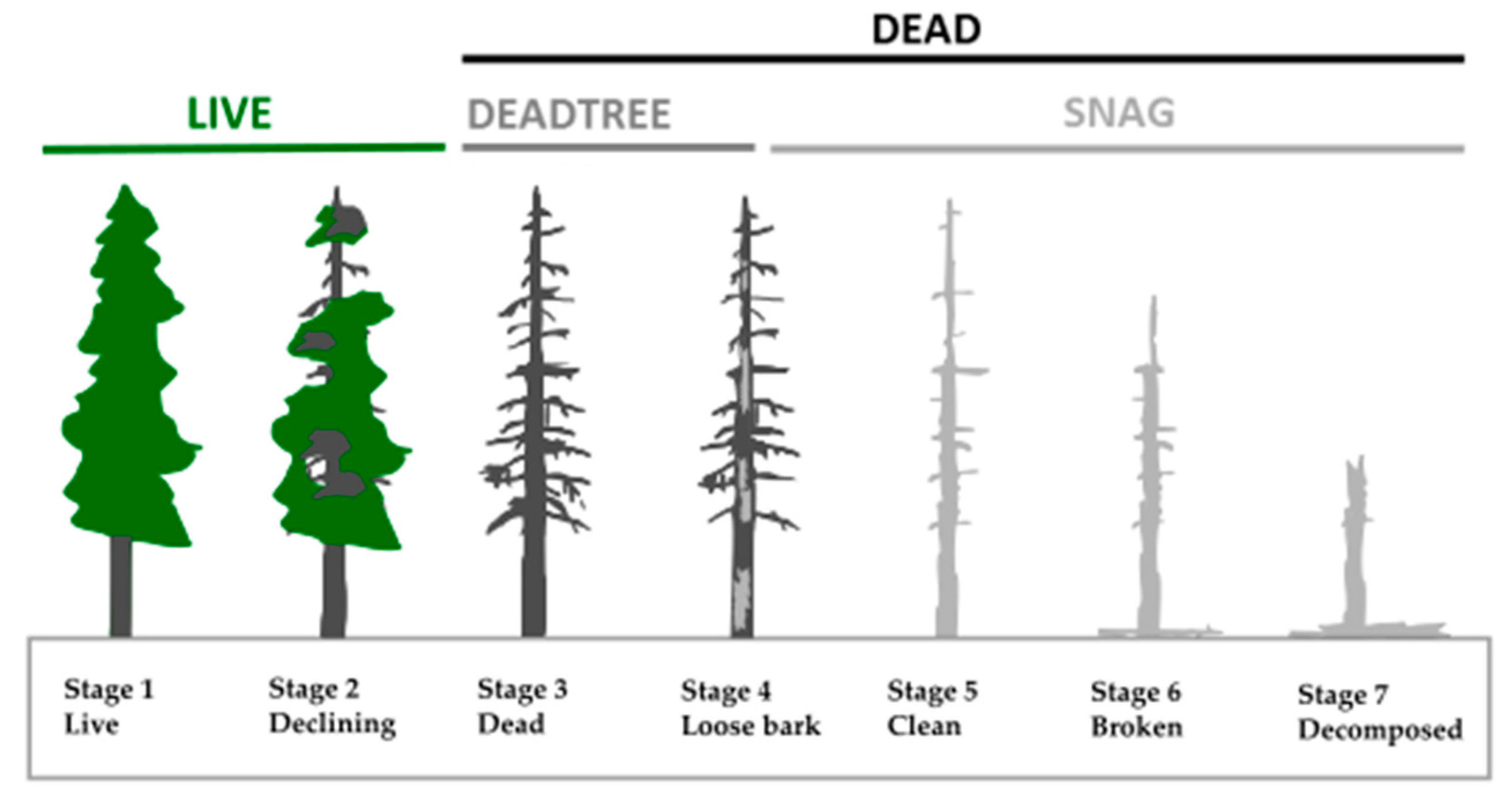
| DEAD_Cmean | Mean crown area of all standing deadwood per plot | Feeding potential for BB/Option for cavities | m2 | |
| SNAG_Nha | Amount of snags per ha | Old deadwood (rather unsuitable) | N/ha | |
| SNAG_Hmean | Snags mean height per plot | Old deadwood (rather unsuitable) | m | |
| SNAG_Cmean | Snags mean crown area per plot | Old deadwood (rather unsuitable) | m2 | |
| DEADTREE_Nha | Amount of all standing dead trees per ha | Deadwood with BB potential | N/ha | |
| DEADTREE_Hmean | Mean H of all standing dead trees per plot | Deadwood with BB potential | m | |
| DEADTREE_Cmean | Mean crown area of all standing dead trees per plot | Deadwood with BB potential | m2 | |
| Topography | ALTITUDE_mean | Mean altitude a.s.l. of a sampling plot | Proxy for climate | m |
| SLOPE_mean | Mean slope of a sampling plot | Proxy for terrain | Degree | |
| EAST | Easting (sine of aspect) of a sampling plot | Sun exposure | (−1)–1 | |
| NORTH | Northing (cosine of aspect) of a sampling plot | Sun exposure | (−1)–1 | |
| SOLAR_mean | Yearly mean of solar radiation per plot | Proxy for climate | h |
| R = 100 m | R = 250 m | R = 450 m | R = 600 m | |||||
|---|---|---|---|---|---|---|---|---|
| Variables p < 0.05/0.1 | Linear | Quadratic | Linear | Quadratic | Linear | Quadratic | Linear | Quadratic |
| Altitude_mean | 0.040 | 0.042 | 0.043 | 0.045 | ||||
| CONIF_Nha | 0.063 | 0.025 | 0.031 | |||||
| DEAD_Cmean | 0.003 | 0.006 | 0.028 | 0.096 | ||||
| DEADTREE_Nha | 0.025 | 0.000 | 0.034 | 0.005 | 0.035 | 0.066 | 0.091 | 0.089 |
| SNAG_Cmean | 0.052 | 0.043 | 0.063 | |||||
| LIVE_Nha | 0.081 | 0.076 | 0.07 | |||||
| CONIF_VOLpart | 0.051 | 0.096 | ||||||
| DEADCIR_part | 0.007 | 0.064 | ||||||
| R = 100 m | R = 250 m | R = 450 m | R = 600 m | |||||
|---|---|---|---|---|---|---|---|---|
| edf | p-Value | edf | p-Value | edf | p-Value | edf | p-Value | |
| Intercept estimate | 0.134 | 0.035 | 0.013 | 0.006 | ||||
| Standard error | 0.249 | 0.227 | 0.208 | 0.205 | ||||
| Z-Value | 0.537 | 0.156 | 0.064 | 0.032 | ||||
| Pr(>|z|) | 0.591 | 0.876 | 0.949 | 0.975 | ||||
| s(Altitude_mean) | 0.817 | 0.049 | 0.929 | 0.020 | 0.681 | 0.076 | 0.605 | 0.105 |
| s(DEAD_Cmean) | 0.167 | 0.239 | 0.947 | 0.018 | 0.784 | 0.038 | 0.627 | 0.103 |
| s(DEADTREE_Nha) | 1.000 | 0.000 | 0.906 | 0.007 | 0.953 | 0.021 | 0.855 | 0.027 |
| s(SNAG_Cmean) | 0.790 | 0.099 | ||||||
| s(CONIF_VOLpart) | 0.620 | 0.114 | 1.571 | 0.107 | 0.176 | 0.252 | ||
| te(x,y) | 1.795 | 0.045 | 1.742 | 0.154 | 1.509 | 0.033 | 1.640 | 0.037 |
| R = 100 m | R = 250 m | R = 450 m | R = 600 m | |||||||||
|---|---|---|---|---|---|---|---|---|---|---|---|---|
| Model Fit | CV | Model Fit | CV | Model Fit | CV | Model Fit | CV | |||||
| Mean | SD | Mean | SD | Mean | SD | Mean | SD | |||||
| R-sq.(adj.) | 0.33 | 0.34 | 0.04 | 0.25 | 0.25 | 0.06 | 0.14 | 0.15 | 0.04 | 0.11 | 0.12 | 0.03 |
| AUC | 0.85 | 0.77 | 0.10 | 0.82 | 0.71 | 0.08 | 0.74 | 0.63 | 0.09 | 0.72 | 0.61 | 0.10 |
| Sensitivity | 0.85 | 0.75 | 0.14 | 0.83 | 0.66 | 0.06 | 0.75 | 0.58 | 0.13 | 0.71 | 0.54 | 0.07 |
| Specificity | 0.73 | 0.67 | 0.24 | 0.69 | 0.65 | 0.13 | 0.64 | 0.52 | 0.17 | 0.60 | 0.58 | 0.12 |
| CCR | 0.79 | 0.71 | 0.12 | 0.76 | 0.65 | 0.08 | 0.69 | 0.55 | 0.12 | 0.65 | 0.56 | 0.06 |
| Cohen’s Kappa | 0.58 | 0.41 | 0.24 | 0.52 | 0.31 | 0.15 | 0.39 | 0.10 | 0.24 | 0.31 | 0.12 | 0.12 |
© 2018 by the authors. Licensee MDPI, Basel, Switzerland. This article is an open access article distributed under the terms and conditions of the Creative Commons Attribution (CC BY) license (http://creativecommons.org/licenses/by/4.0/).
Share and Cite
Zielewska-Büttner, K.; Heurich, M.; Müller, J.; Braunisch, V. Remotely Sensed Single Tree Data Enable the Determination of Habitat Thresholds for the Three-Toed Woodpecker (Picoides tridactylus). Remote Sens. 2018, 10, 1972. https://doi.org/10.3390/rs10121972
Zielewska-Büttner K, Heurich M, Müller J, Braunisch V. Remotely Sensed Single Tree Data Enable the Determination of Habitat Thresholds for the Three-Toed Woodpecker (Picoides tridactylus). Remote Sensing. 2018; 10(12):1972. https://doi.org/10.3390/rs10121972
Chicago/Turabian StyleZielewska-Büttner, Katarzyna, Marco Heurich, Jörg Müller, and Veronika Braunisch. 2018. "Remotely Sensed Single Tree Data Enable the Determination of Habitat Thresholds for the Three-Toed Woodpecker (Picoides tridactylus)" Remote Sensing 10, no. 12: 1972. https://doi.org/10.3390/rs10121972