A New Method for Region-Based Majority Voting CNNs for Very High Resolution Image Classification


1
School of Information Engineering, China University of Geosciences (Beijing), 29 Xueyuan Road, Beijing100083, China
2
Key Laboratory of Virtual Geographic Environment (Nanjing Normal University), Ministry of Education, Nanjing 210046, China
*
Author to whom correspondence should be addressed.
Remote Sens. 2018, 10(12), 1946; https://doi.org/10.3390/rs10121946
Submission received: 15 November 2018
/
Revised: 29 November 2018
/
Accepted: 30 November 2018
/
Published: 4 December 2018
(This article belongs to the Special Issue Region Based Classification (RBC), Object Based Image Analysis (OBIA) and Deep Learning (DL) for Remote Sensing Applications)
Abstract
:Conventional geographic object-based image analysis (GEOBIA) land cover classification methods by using very high resolution images are hardly applicable due to their complex ground truth and manually selected features, while convolutional neural networks (CNNs) with many hidden layers provide the possibility of extracting deep features from very high resolution images. Compared with pixel-based CNNs, superpixel-based CNN classification, carrying on the idea of GEOBIA, is more efficient. However, superpixel-based CNNs are still problematic in terms of their processing units and accuracies. Firstly, the limitations of salt and pepper errors and low boundary adherence caused by superpixel segmentation still exist; secondly, this method uses the central point of the superpixel as the classification benchmark in identifying the category of the superpixel, which does not allow classification accuracy to be ensured. To solve such problems, this paper proposes a region-based majority voting CNN which combines the idea of GEOBIA and the deep learning technique. Firstly, training data was manually labeled and trained; secondly, images were segmented under multiresolution and the segmented regions were taken as basic processing units; then, point voters were generated within each segmented region and the perceptive fields of points voters were put into the multi-scale CNN to determine their categories. Eventually, the final category of each region was determined in the region majority voting system. The experiments and analyses indicate the following: 1. region-based majority voting CNNs can fully utilize their exclusive nature to extract abstract deep features from images; 2. compared with the pixel-based CNN and superpixel-based CNN, the region-based majority voting CNN is not only efficient but also capable of keeping better segmentation accuracy and boundary fit; 3. to a certain extent, region-based majority voting CNNs reduce the impact of the scale effect upon large objects; and 4. multi-scales containing small scales are more applicable for very high resolution image classification than the single scale.

1. Introduction
With the development of remote sensing sensor technology such as WorldView 4 (WV-4), GaoFen-2, SuperView-1 etc., the spatial resolution of remote sensing images has been increasing year by year. More and more very high resolution images (VHRI) have been obtained and widely used in many fields, such as in natural sources management [1,2,3], urban mapping [4] and military reconnaissance. VHRI contains extremely rich information, according to which some simple features can be extracted and selected as basic features to classify categories in VHRI. Meanwhile, plenty of information hidden in the deep features of VHRI cannot be effectively distinguished and fully exploited for image classification and geo-application.
VHRI classification, including urban image classification and agriculture image classification, is an important field of remote sensing. Geographic object-based image analysis (GEOBIA) is devoted to developing automated methods to partition remote sensing imagery into meaningful image-objects [5,6] and assessing their characteristics through spatial, spectral, and temporal scales to generate new geographic information in a GIS-ready format. A great deal of progress has been made in the field of GEOBIA; however, the classification features need to be manually selected before they are put into the classifier for classification. Traditional classifiers such as the Bayesian classifier [7,8,9,10,11], support vector machine [12,13,14,15], and some other classification methods with contextual information [16,17,18] have good performance for low resolution image applications. The commonly used shallow features, such as geometrical, textural, and contextual information, are without exception perceptible with the human eye [19]. In contrast, the deep features which cannot be effectively extracted by traditional methodology play little role in VHRI classification by traditional GEOBIA methods [20]. In recent years, deep learning [21] has made a great deal of progress in image processing, as well as in remote sensing image classification [22]. In addition, the effectiveness of convolutional neutral networks (CNNs) in automatic road detection [23], scene classification [24,25], vehicle type classification [26] and object detection [27] has been practically proved. All of this progress benefits from CNNs’ capability for extracting deep features hidden in VHRI [28].
To solve the deep feature extraction problems, pixel-based CNN (pixel-CNN) is being introduced into remote sensing classification [20,29,30,31,32,33,34] with the advent of deep learning. With multiple deep hidden convolutional layers and pooling layers, CNN can extract deep features effectively from VHRI. Pixel-CNN exhibits better performance in extracting deep features than other methods and can provide higher classification accuracy because of the robustness of deep feature learning. Furthermore, based on pixel-CNN, the performance of multi-scales is proven to be better than that of the single scale for most remote sensing images [20]. However, a large amount of running time and a huge amount of disk space are required by pixel-CNN when using a sliding window to process the whole image.
A superpixel-based CNN (superpixel-CNN) algorithm is proposed to overcome the troubles mentioned above [35,36,37]. A superpixel is an over-segmented patch with high homogeneity [38,39,40,41] and is gradually being applied to the field of GEOBIA. Competitively compared with pixel-CNN, the computational time has been greatly reduced and the spatial processing units have been decreased sharply by using superpixel-CNN [36]. Additionally, in some situations, e.g., for extremely complex images, a single-scale classification result of CNNs performs better than that of multi-scale. However, for the majority of remote sensing images, a multiple scale classification accuracy is higher than a single scale [42].
Currently, there are about 30 superpixel segmentation methods, including good boundary fitting segmentation methodologies such as multiresolution segmentation, mean shift, and watershed algorithm and gradient descent-based superpixel segmentation algorithms [43] such as linear spectral clustering, simple linear iterative clustering, and superpixels extracted via energy-driven sampling. According to the structure and theory of CNNs, a restriction is required: the training data to be fed into the input layer of the CNN must be fixed size image. Thus, the superpixel segmentation method applied to the superpixel-CNN should keep a good balance between boundaries and compactness. Not all segmentation methods can be used for superpixel-CNN. Only superpixel segmentation with good performance for boundaries and compactness are available for superpixel-CNN such as the superpixels extracted via energy-driven sampling CNN (SEEDS-CNN) method which performs best compared with other superpixel-based CNN methods [44]. Otherwise, due to the compactness limitation of superpixels, the classification result boundaries within categories inevitably introduce some errors, which are intra-class superpixels. The CNN has a high robustness for the deep features extraction of categories and the interior of the classified patch has few errors because of its high homogeneity. Thus, the key to image classification depends on the classification accuracies surrounding patch boundaries. However, superpixel-CNN performs worse at the boundary area owing to the limitations mentioned above. Solving the boundary problems of superpixel-CNN-based remote sensing image classification has become increasingly important.
Good boundary fitting segmentation methods include multiresolution segmentation (MRS) [45], mean shift [46], entropy rate superpixel [39], and so on. However, good boundary fitting segmentation does not follow the rules of superpixel segmentation, and although it can generate good performance for boundaries [47], the shapes of over-segmented regions are various, which results in it being incapable of ensuring the region classification accuracy when only the central point of the region is used as the benchmark in category identification. Thus, to solve the related problems, it is a good approach to combine the boundary advantage of good boundary fitting segmentation with a majority voting strategy into region-based multi-scale CNN classification.
A new method named region-based majority voting CNN (RMV-CNN) was proposed to solve the boundary problem. RMV-CNN introduces good boundary fitting segmentation into multi-scale CNN image classification through a new majority voting strategy to overcome the limitation of region shape for CNNs. Thus, on the one hand, the computational efficiency can be greatly improved by reducing the number of spatial processing units to about one hundredth of those of pixel-CNN, so that a large amount of computational time and hard disk space can be saved; on the other hand, the boundary errors caused by superpixel-CNN can be avoided in some situations, and the overall accuracy of the RMV-CNN image classification results is about 2% or even 4% higher than SEEDS-CNN. The selection of good boundary fitting segmentation methods for CNN is not only good for keeping a balance between boundaries and compactness, but also focuses on the boundary performance, which is the key issue for VHRI classification.
The remainder of this paper is organized as follows. The principle and related algorithms are described in Section 2. The effectiveness of the proposed RMV-CNN method was tested on three images of large urban and agricultural scenes, and the related data description and the experimental classification results of RMV-CNN, SEEDS-CNN and the center point of the region CNN (center-CNN) are shown in Section 3. The experimental results are analyzed and discussed in Section 4, followed by conclusions being given in Section 5.
2. Method of the Region-Based Majority Voting CNN for VHRI Classification
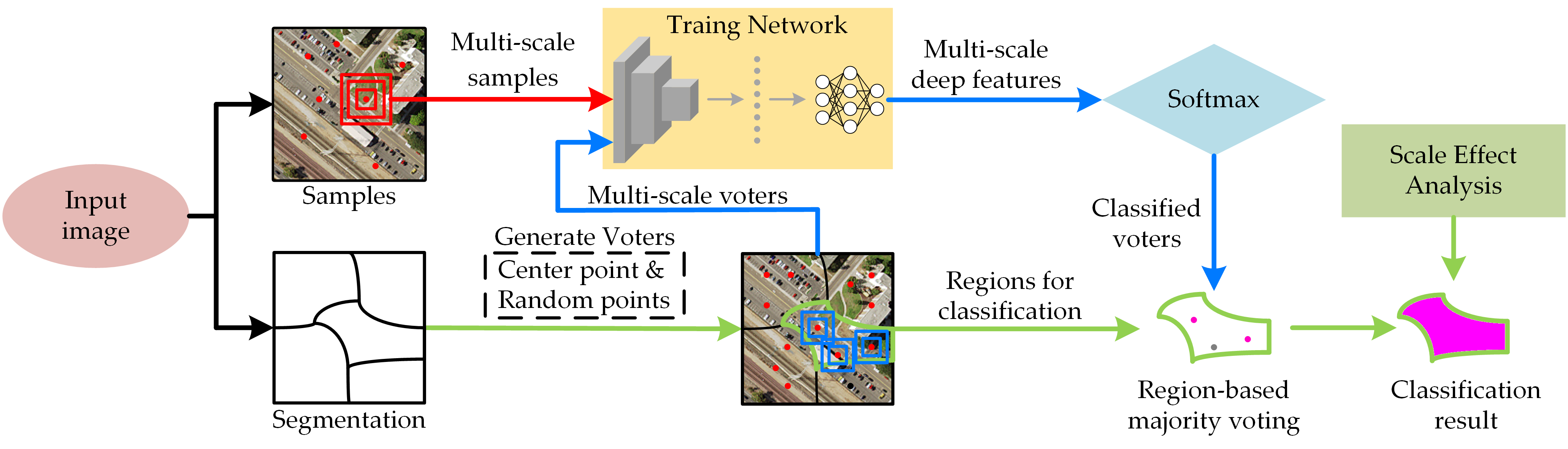
Very similar to superpixel-CNN classification methods, as illustrated in Figure 1, RMV-CNN contains three steps: segmentation for VHRI, the training CNN model, and majority voting for image classification.
In the segmentation for VHRI, the experimental image is segmented into many different regions, which are the basic spatial processing units with high homogeneity. There are many segmentation methods available, such as MRS, the watershed algorithm, mean shift, and so on. In fact, all of the segmentation algorithms with a good edge fit can be employed for RMV-CNN.
In the training CNN, the CNN is fed by the labeled data extracted from the image. The CNN is adjusted to have more robustness for extracting complicated and effective deep features by continuous step-by-step training. After training the CNN, all of the test data can be classified by the trained CNN. Considering the scale dependence of GEOBIA, this paper uses a multi-scale CNN to extract complex deep features for final classification.
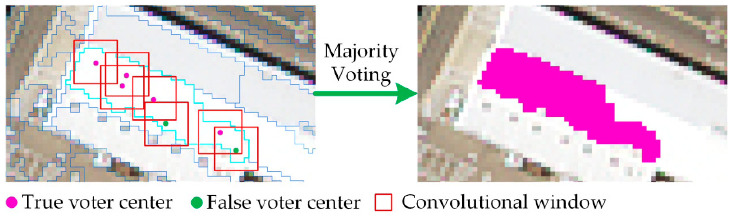
In the final step, each region is labeled by voter data, which is generated by the region majority voting system. There are odd voters in each patch: one is the centroid of the patch, and the others are randomly generated within the patch contour. The final patch classification result depends on the candidate label with the highest number of votes. It is worth emphasizing that both the sample points and the voter points are the convolutional center.
2.1. Convolutional Neural Network (CNN) and AlexNet
Essentially, CNN is a multi-layer perceptron with many hidden convolutional layers and pooling layers [48]. The key issue to its success lies in the fact that it uses local connections and shares weights. On the one hand, the number of weights is reduced, which makes the network easy to optimize. On the other hand, the risk of over-fitting is reduced. The CNN is similar to biological neural networks in essence. The weight-sharing network structure reduces the complexity of the network model and the amount of weights. This advantage is more obvious when the input of the network is a multi-dimensional image. As images can be directly used as inputs of the network, the CNN avoids the complicated feature extraction and data reconstruction process in the traditional recognition algorithms. Besides this, CNN also has many advantages in two-dimensional image processing. For example, the network can extract image features including color, texture, shape and even some image topology. Moreover, in the processing of two-dimensional images, especially in identifying moving, scaling and other forms of distortion invariance, it is good at maintaining robustness and computational efficiency.
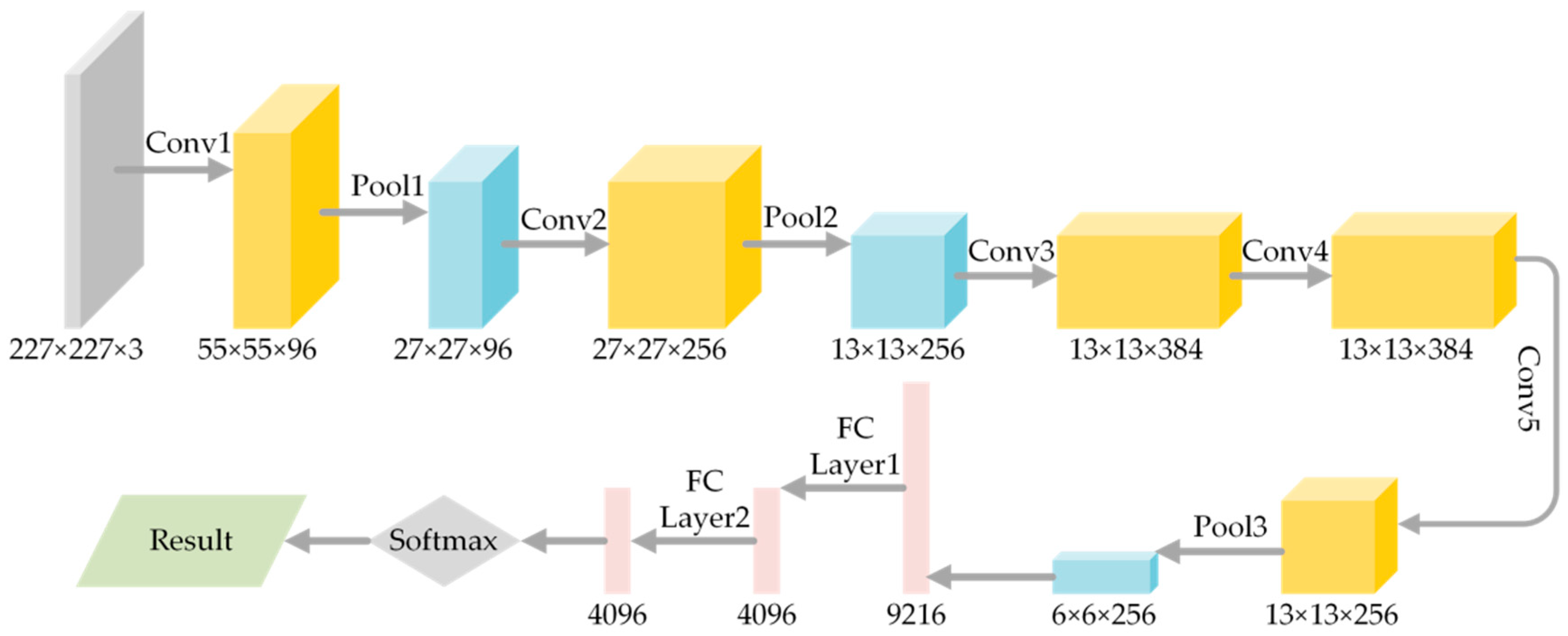
AlexNet, a commonly used framework of CNN, was the winner of the ImageNet Large Scale Visual Recognition Challenge in 2012 [48]. AlexNet contains 5 convolutional layers, 3 pooling layers and 2 fully-connected layers. However, it only supports images with 3 bands. Different numbers of filters used for extracting features are applied in each convolutional layer. Also, the activation function of AlexNet used for controlling the range of values is rectified linear units (ReLU), which is the function . In fact, the contribution of convolutional layers and pooling layers is used as a feature extractor. The features extracted by convolutional layers from the image form a feature map. The fully-connected layers convert feature maps into image feature vectors supported by general classifiers. Softmax is applied as a classifier to classify the extracted deep features. Figure 2 depicts the network structure of AlexNet.
2.2. Multiresolution Segmentation (MRS)
The basic thought behind multiresolution segmentation (MRS) is the fractal net evolution approach (FNEA) [45]. In a given resolution, objects of different scales exist simultaneously, which generates a hierarchical level network of image objects. At each hierarchical level, MRS performs a bottom-up region growing segmentation based on pixels, which abides by the minimum heterogeneity principle and merges spectrally similar neighbors which are given the same label after segmentation. The segmentation considers not only spectral features but also other figurative features; therefore, the heterogeneity comprises two aspects, spectral homogeneity and shape homogeneity. The underlying aim of this algorithm is to gain the minimum heterogeneity after every mergence, and thus an image object ought to be absorbed into a new object whose heterogeneity is the lowest among potential candidates. Consequently, the homogeneity of two objects is defined by Equation (1):
where h1 and h2 are the heterogeneities of two objects before merging; hm is the heterogeneity of the newly generated object, calculated by Equation (2); and hdiff is the heterogeneity difference before and after merging.
where d means the d-dimension, which is the band number; and f1d and f2d mean spectral values or texture features, such as the variance of spectral values.
However, when the sizes of objects and the possible influence of bands are taken into consideration, hdiff can be further determined by Equation (3):
where wc is the weight of different bands and n1 and n2 are the pixel amounts of each object; h1c and h2c are, respectively, the heterogeneities of the two original objects in different bands; and hmc is the heterogeneity of the newly generated object in different bands. As mentioned above, the MRS considers spectral, spatial and figurative features in segmentation. Accordingly, the heterogeneity is synthetically determined by spectral and figurative (or shape) heterogeneity. The final Equation (4) is demonstrated as follows:
where ωcolor and ωshape are the weights of the spectral and figurative heterogeneity, respectively; hcolor and hdiff in Formula (1) are the same feature; hshape are the spectral heterogeneity and figurative heterogeneity, calculated by Equation (5); and is the upper limit for a permitted change of heterogeneity throughout the segmentation process. Thus, refers to the overall area-weighted homogeneity and determines the sizes of segmented regions.
where l is the edge length and n is the object size in pixels.
2.3. Region Voters Generation
Region point voters for majority voting contain two categories. One is the center point of this region and other voters are an even number of randomly generated points within this region.
2.3.1. Center Points Generation
Central points within each polygon are generated by Equation (4). For a non-self-crossing polygon, let given vertices be V1, V2, …, Vn and represented as vector quantities. The center point shall be as Equation (6):
where C is the center point and Vi denotes each vertex. Therefore, the procedure can be described as follows: 1. the vector (Vi) of each vertex is calculated according to coordinates; 2. Vi is determined to obtain Sum(Vi); 3. the vector of the center point is generated, Vc = Sum(Vi)/n; 4. Finally, the coordinate of the center point is generated based on Vc.
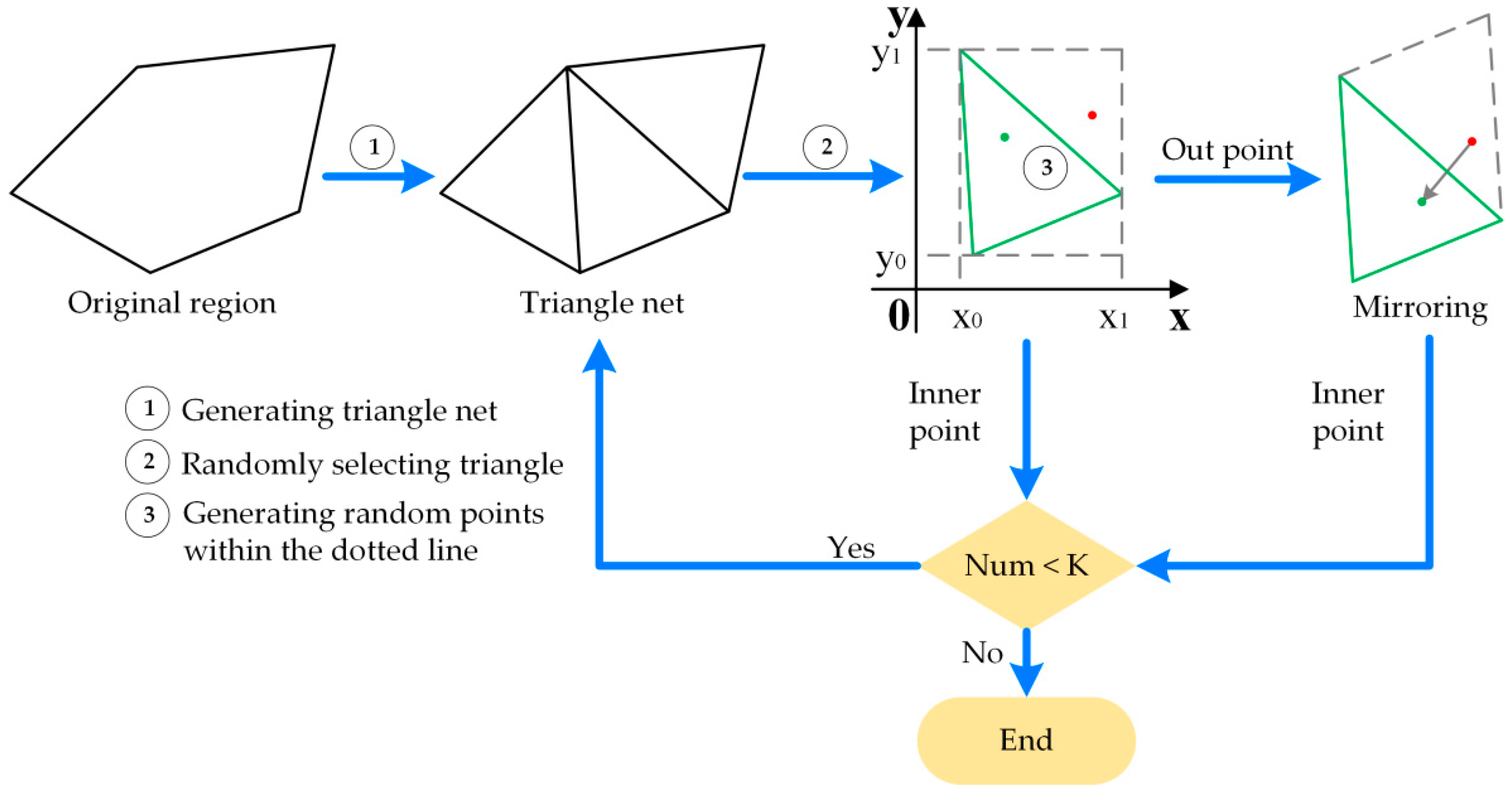
2.3.2. Random Points Generation
A specified amount of random points can be obtained within a certain polygon or line. The first step is to create a random number stream via a random number builder and seeds. The polygon would be partitioned into a specified number of triangles, within which lies a random point. When a random point is generated within a specified range, the random values of the range are identified on the x-axis and y-axis, respectively, as shown in Figure 3, and these values become the x-coordinates and y-coordinates of the point. To randomly select a point on the x-axis, the next unused value in the random number data stream is selected and transformed into a “uniform” distribution, where the minimum and maximum values are the minimum and maximum values of the x-range, respectively. The same operation is then performed on the y-axis. The two random values obtained identify the first random point. This process will be repeated until the number of points is reached.
Two sides of a triangle are taken as the x-axis and y-axis on which random numbers are generated and used as coordinates. If the point, however, is generated outside the triangle, it shall be mirrored into the triangle. Thus, all the points are generated randomly within the polygon. The procedure will be iteratively performed until all required points are obtained. The workflow is shown in Figure 3.
2.4. Region-Based Majority Voting Strategy
After the voter data is labeled by the pre-trained CNN, each voter point in the patch has a unique classification. The patch classification shows the label with the most votes. Because each segmented patch has high homogeneity, the voters in the patch almost have the same classification labels, except for some extreme situations. Therefore, the voting result is trustworthy. Some of the voters in a position with complicated land cover may be incorrectly classified. Other voters at the same patch will classify the true label for the patch, avoiding the influences by the particular incorrect voter. Therefore, with the conception of majority voting, RMV-CNN has much more robustness for image patch classification. The process of majority voting is shown in Figure 4.
2.5. Overall Accuracy Assessment Method
The overall accuracy of the final classification results is based on the error matrix, which is also known as the confusion matrix. It is used to validate the precision of a certain type of object points in matching the ground truth. Generally, columns in the matrix represent reference data, while rows are classification results. The result is usually shown as a pixel amount and as a percentage. The total pixels were divided by the correctly classified pixels to generate the overall accuracy. The numbers of correctly classified pixels were listed along the diagonal line of the error matrix, while the number of total pixels equals the number of all pixels with the true reference source. The calculation of the Kappa coefficient is given by Equation (7):
where K is the Kappa coefficient; P0 is the overall classification accuracy; and Pe is the agreement expected on the basis of chance. P0 is obtained via dividing the total samples by each type of correctly classified samples. Let the number of each type of samples be a1, a2, …, ac, the predicted number of each type be b1, b2, …, bc, and the number of total samples be n; then, Pe = (a1 × b1 + a2 × b2 + …+ ac × bc)/(n × n).
3. Experiments
In this section, there are two main parts. Section 3.1 is about the data description and preprocessing. To verify the effectiveness of the proposed RMV-CNN method, Section 3.2 compares the experimental VHRI classification results by RMV-CNN with those by SEEDS-CNN and center-CNN. Thanks to its impressive ability to extract deep features, AlexNet was utilized as the foundation CNN frame. Experiments were carried out on Ubuntu16.04 OS with a CPU (3.4 GHz core i7-6700), RAM (8 GB), and a GPU (NVIDIA GTX 1050 2 GB). TensorFlow was chosen as the deep learning platform.
3.1. Study Area and Data Pre-Processing
3.1.1. Description of Images
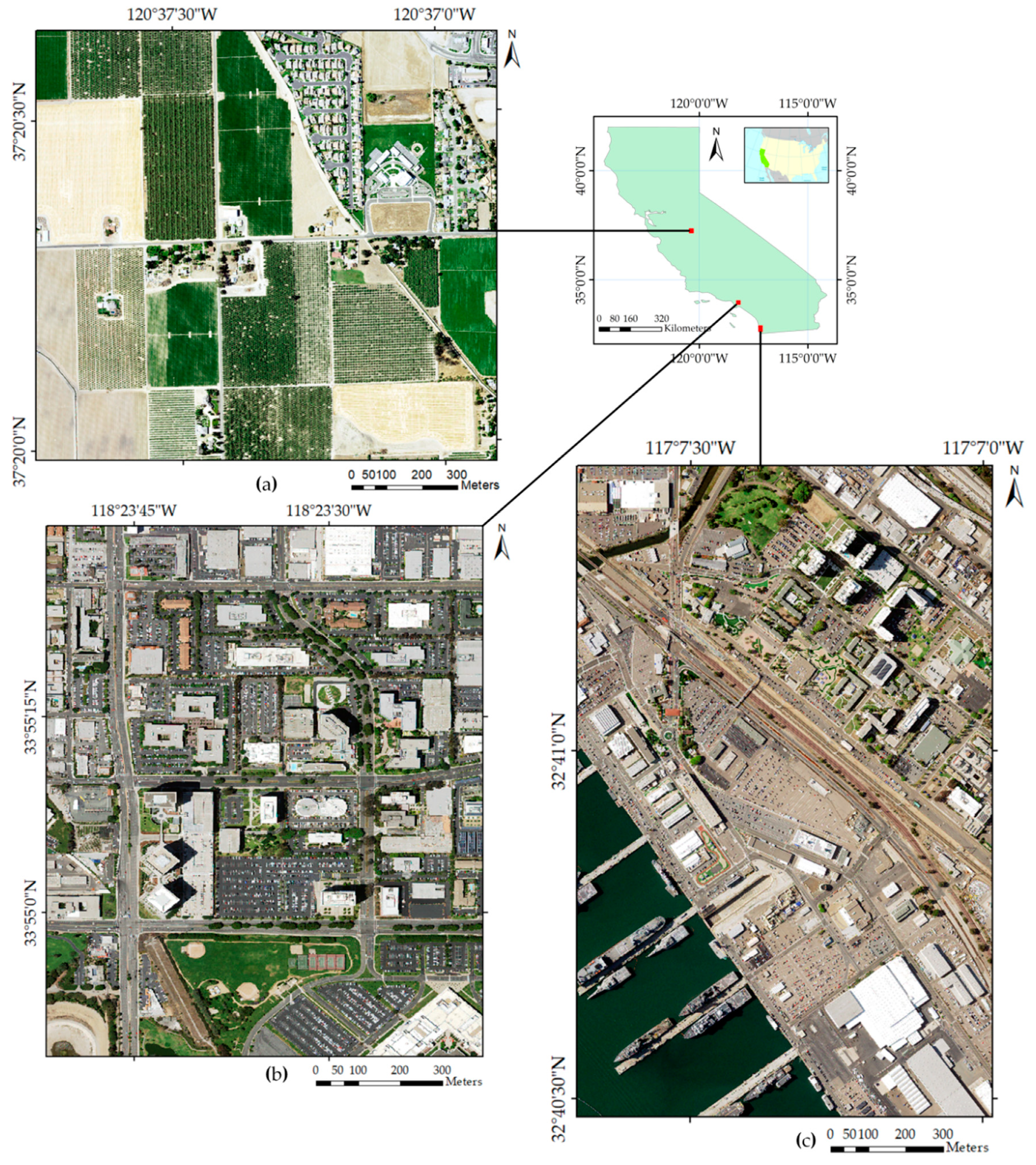
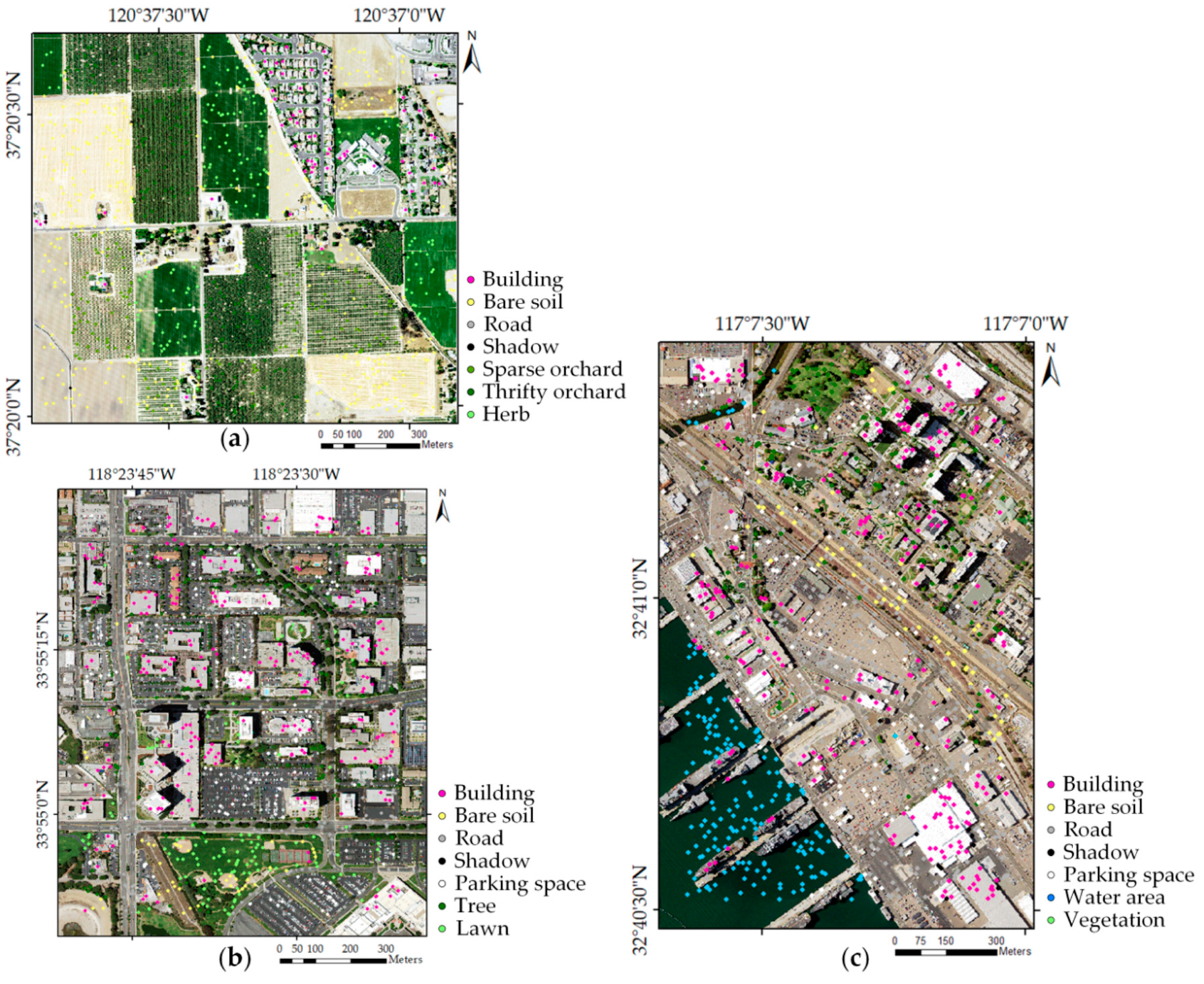
In this paper, as shown in Figure 5, experimental images with 1 m spatial resolution are from Digital Orthophoto Quarter Quad, which are provided by the National Agriculture Imagery Program of the United States Department of Agriculture. Images captured in summer which could provide rich vegetation information were chosen for experiments. Urban land cover classification and agriculture crop classification are important applications of very high resolution remote sensing images. Thus, three images covering urban areas and agricultural areas were selected for the experiments. Figure 5a is an agricultural area located in the city of Atwater of California. There are various types of agricultural land cover in the Atwater image. Figure 5b, the EI Segundo image, is located in the southwest of Los Angeles, California and covers a commercial region that is composed of complex objects, such as buildings with different heights and shapes, asphalt roads with high homogeneity, large lawns and scattered trees. Figure 5c is an image from San Diego, California, America. In the San Diego image, there are many buildings, roads and some water areas.
The three experimental images contain 4 bands including red (R), green (G), blue (B) and near infrared (NIR), while the training data for CNN can contain only 3 bands. Therefore, these 4 bands were selected and combined to form the best combination for the CNN by using the optimal index factor (OIF) [49]. OIF is a classical band selection method which considers the amount of information from each band and the correlation among different bands. The input training data was formed by selected bands. The OIF can be calculated by Equation (8):
where Si is the standard deviation of the ith band of the image and Rij is the correlation coefficient between the ith band and jth band at the same time.
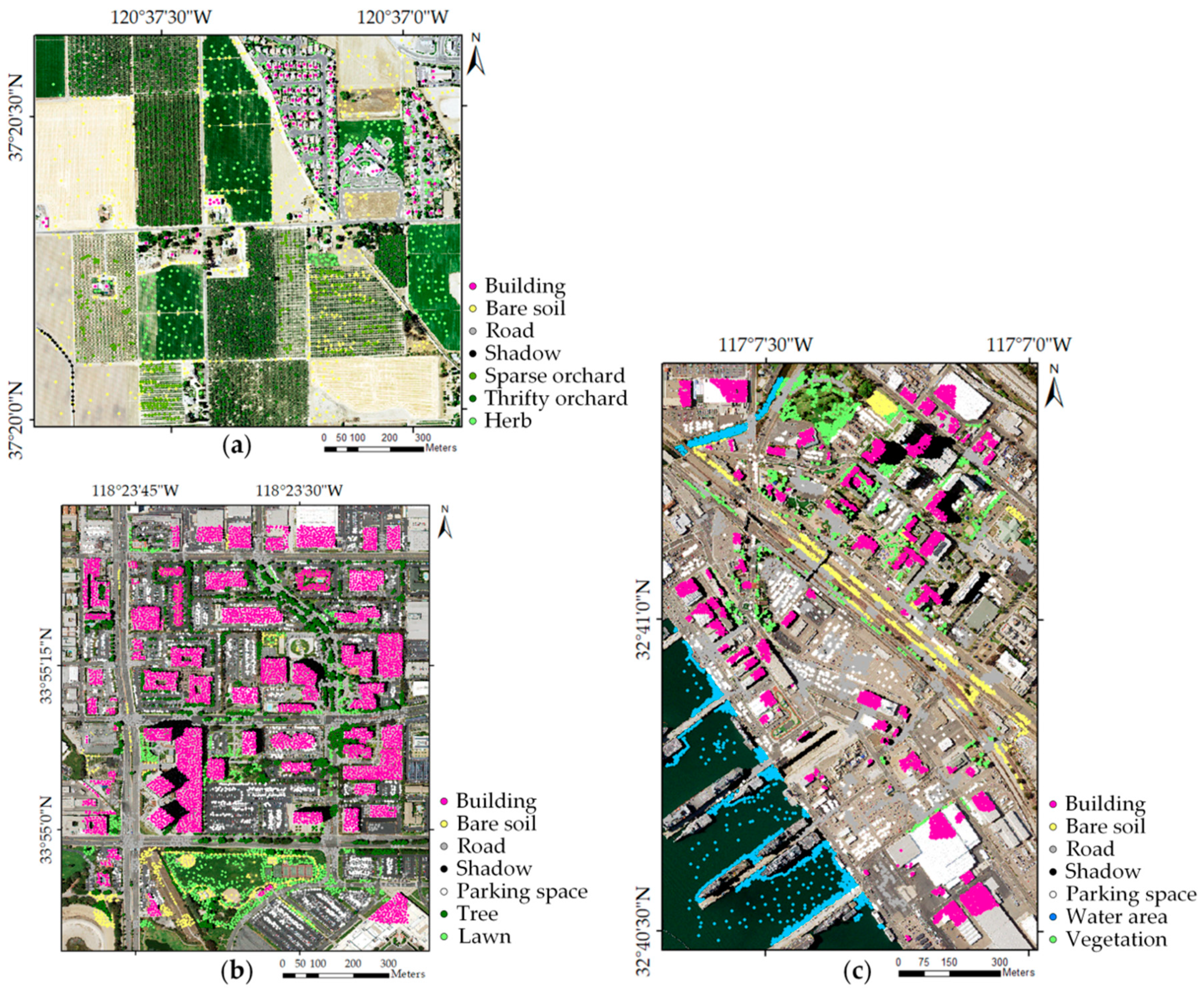
After analyzing the land cover categories contained in the images from Atwater, EI Segundo and San Diego, four categories (building, road, bare soil and shadow) simultaneously exist in the three images. Buildings and roads are the main objects of urban images. Their classification is both a key point and a difficult point. Bare soil is an important indicator for monitoring urban dust. There are hardly any trees in the image from San Diego; however, there are many obvious trees in the EI Segundo image, and so the green vegetation of EI Segundo is further separated into trees and lawns. For the Atwater image, the vegetation is classified into three categories, which are sparse orchard, thrifty orchard and herb (grass and low crop). In the orchard, due to the difference in solar light intensity requirements of fruit trees, some fruit trees can be planted more densely (thrifty orchard), and some fruit trees need to be planted sparsely (sparse orchard). Low crops are difficult to distinguish from grass in Atwater. Therefore, both are divided into herbs. Related information about these three images is shown in Table 1 in detail.
3.1.2. Training Data Sampling
Training samples greatly influence the experimental results. Figure 6 shows that these three images, respectively, cover urban districts or agricultural districts with many complex objects. Among those categories, buildings, roads, water areas and parking spaces are dominant in urban images. Sparse orchards, thrifty orchards, herbs and bare soil are dominant in agricultural images. However, the image from EI Segundo is slightly different from San Diego. Firstly, its green space area is more extensive and there is an evident distinction between tree and lawn objects. Secondly, the shapes of roads and parking spaces are easy to be classified compared with the San Diego image. Therefore, the object categories of EI Segundo include buildings, roads, bare soil, shadows, trees and other vegetation. The samples are semi-randomly selected within each object for each category. However, the number of samples of each category is based on the proportions of each types and the complexity of each category to minimize the over/under-representation of training samples per target category. As proportions of certain types of objects are low, more samples of those categories were selected to ensure that the CNN has suitable training samples to learn their features, avoiding CNN over-fitting/under-fitting. On the contrary, objects with high proportion would have their samples relatively reduced. The complexity of agricultural images is lower than urban images. Thus, the number of Atwater samples is significantly lower than urban images.
On the one hand, all categories in the image should be considered. On the other hand, to ensure the appropriate number of samples of each category, samples were semi-randomly selected. Sample points were then taken as convolutional center points. As the experiment considers quite a few extracting scales, which are also known as convolutional window sizes, only locations of sample points as shown in Figure 6 are demonstrated.
In fact, not all sample points labelled in Figure 6 were applied to train the CNN. To enhance the robustness of the CNN, for Atwater and San Diego, 80 percent of the samples were randomly chosen. Fifty percent of the samples of EI Segundo were randomly chosen. The randomly chosen points were divided into training data (80%) and validation data (20%). The validating data considered as a true value are used for calculating the difference between the predicted value and true value. The difference is used for the next epoch to adjust the filters weights of CNN. For each image, the actual samples for training and validation are listed in Table 2.
3.1.3. Parameter Setting for MRS
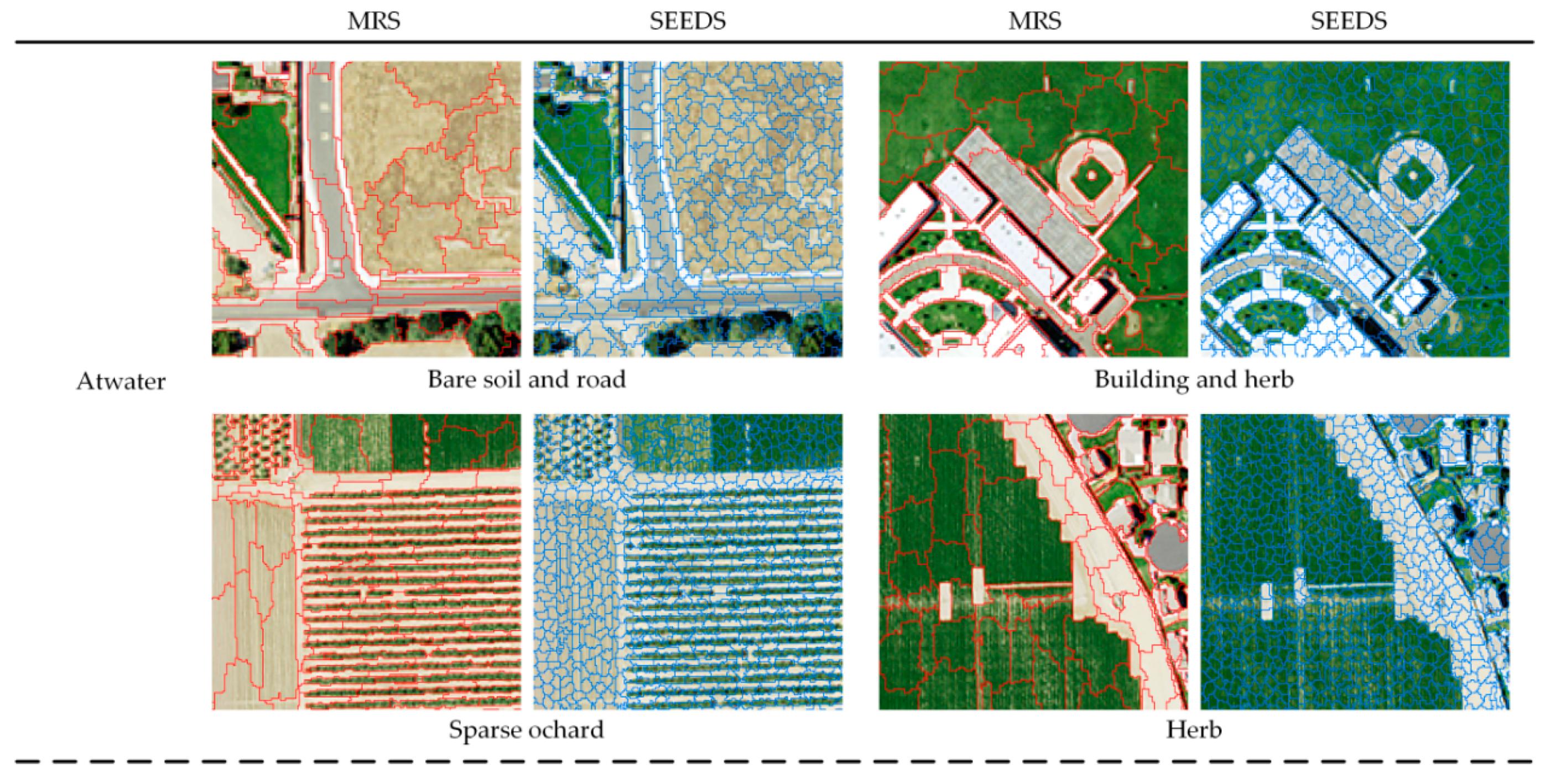
Setting segmentation parameters for the MRS algorithm has an extremely important influence on segmentation results; furthermore, the proposed RMV-CNN is sensitive to the segmented regions. Therefore, the setting of segmentation parameters matters a great deal. Good segmentation will ensure that small objects, e.g., cars, can be segmented and large objects, e.g., buildings, will not be over-segmented. The advantage of MRS lies in that it has a better boundary recall than SEEDS or other superpixel segmentation methods. As described in Section 3.1.1, the categories and their distribution are very different. Thus, segmentation parameters were determined by experience: for the Atwater image, the scale parameter was set as 20, while the shape and compactness values were respectively set as 0.4 and 0.8; for the San Diego image, the scale parameter was set as 20, while the shape and compactness values were respectively set as 0.4 and 0.1; for the EI Segundo image, the scale parameter was set as 15, while the shape and compactness values were set as 0.2 and 0.4, respectively.
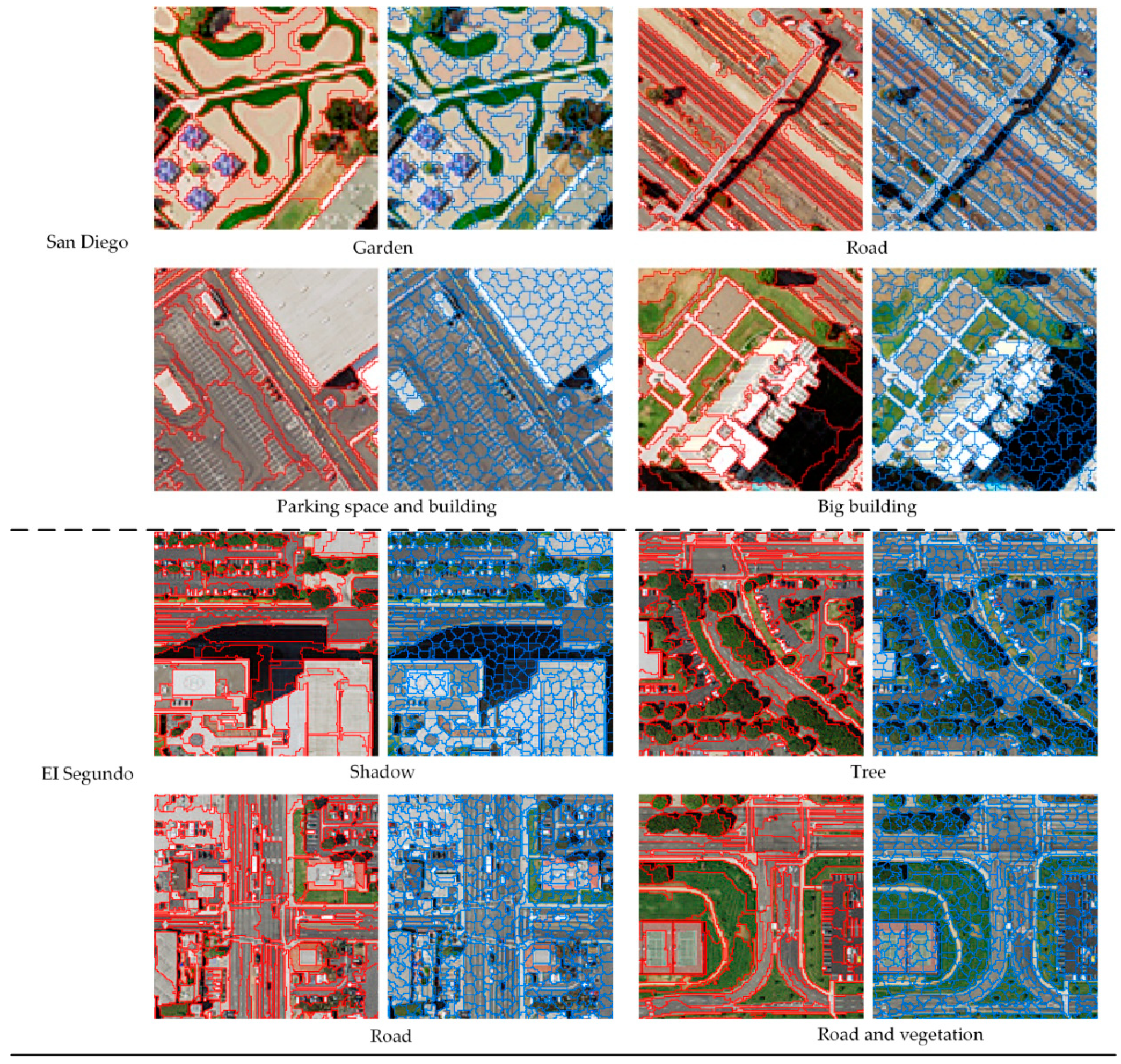
AS the segmentation results cannot be shown clearly here, this paper only demonstrates part of the local segmentation results generated by the MRS and the SEEDS for comparison. Figure 7 shows the local results of segmentation.
3.1.4. Parameters Setting for AlexNet
AlexNet was introduced to the experiment as the fundamental CNN framework. Some parameters for training a CNN need to be clearly stated. For training a single-scale CNN model, the learning rate controlling the learning model progress is 0.01. When a complete data set passes through the neural network and returns once, this process is called an epoch. The number of epochs of this used framework is 60. When data cannot pass through the neural network at once, it is necessary to divide the data set into several batches with a size of 100. So, the number of batches is the training data number divided by the batch size. Avoiding the over-fitting of CNN, the dropout rate is set as 0.5. For training a multi-scale CNN model which mainly retrains its fully-connected layers, the number of epochs is 100; other parameters are the same as the single CNN model.
3.1.5. Overall Accuracy Assessment Points
To truthfully reflect the classification results, it is necessary to ensure that training samples and assessment data are mutually independent. In this experiment, over 1000 random accuracy assessment points were generated independently in each image. These 1000 random accuracy assessment points are different from the validation data in 3.1.2 data sampling. These 1000 points are used for assessing the accuracy of the final classification result. Eventually, the confusion matrix was obtained by comparing the labeled ground truth points and the classification results. Figure 8 demonstrates the locations of ground truth points.
3.2. Experimental Results
This paper compares the RMVCCN, which is taken as the main research method with SEEDS-CNN and center-CNN, to observe the classification accuracy and scale effect.
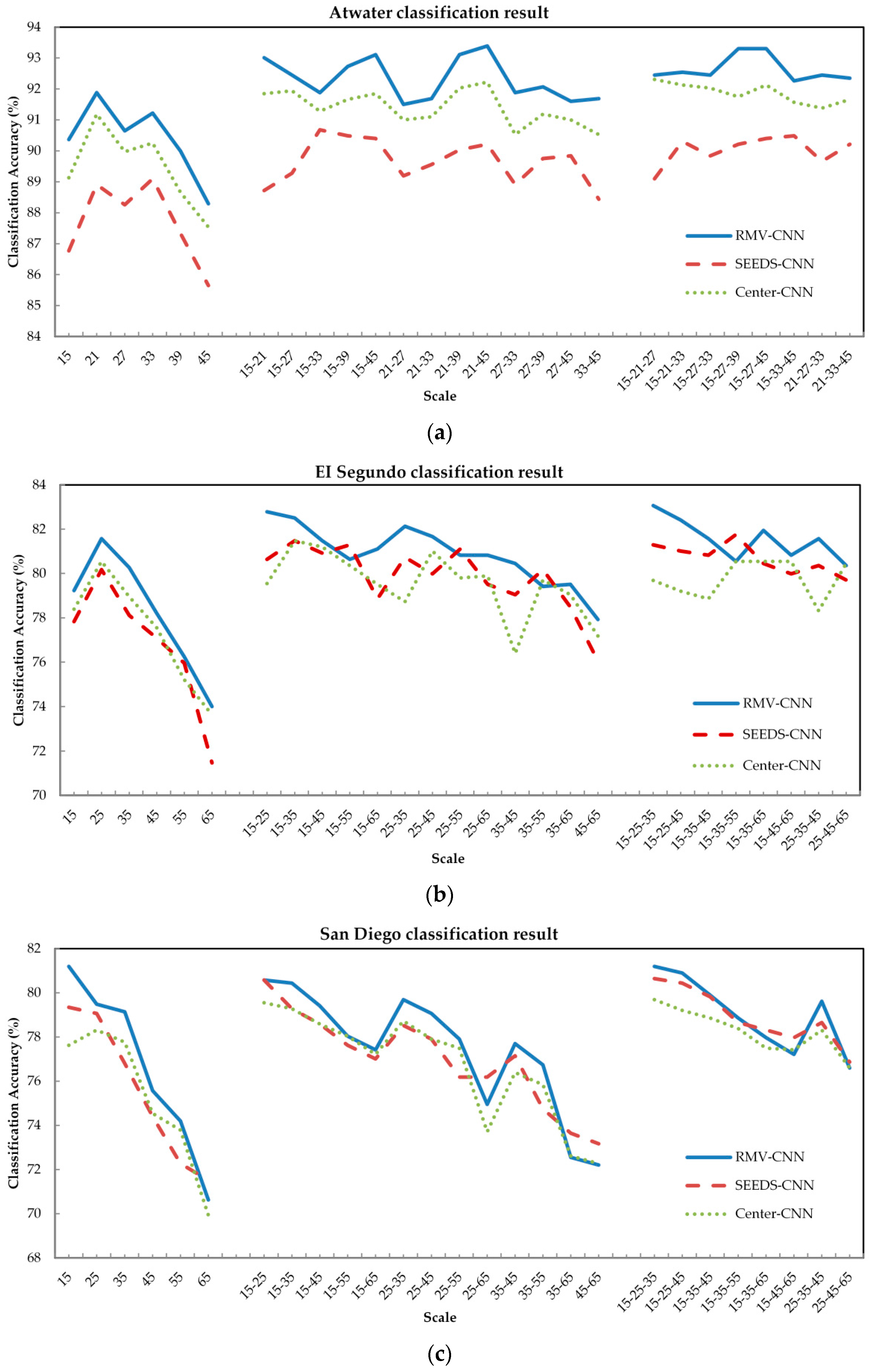
The scale effect is a significant issue in high spatial resolution image classification. As a result, this paper accordingly considers the scale effect. The window sizes, i.e., basic single-scale, were set as 15, 25, 35, 45, 55, and 65, respectively, for urban images. Different to the situation of urban images, the basic single-scales of Atwater were set as 15, 21, 27, 33, 39, and 45. All scales/scale combinations are based on the single-scales. All in all, 27 scales/scale combinations were involved in the experiments, and three methods in this paper were performed and analyzed at these 27 scales.
3.2.1. The Overall Classification Result
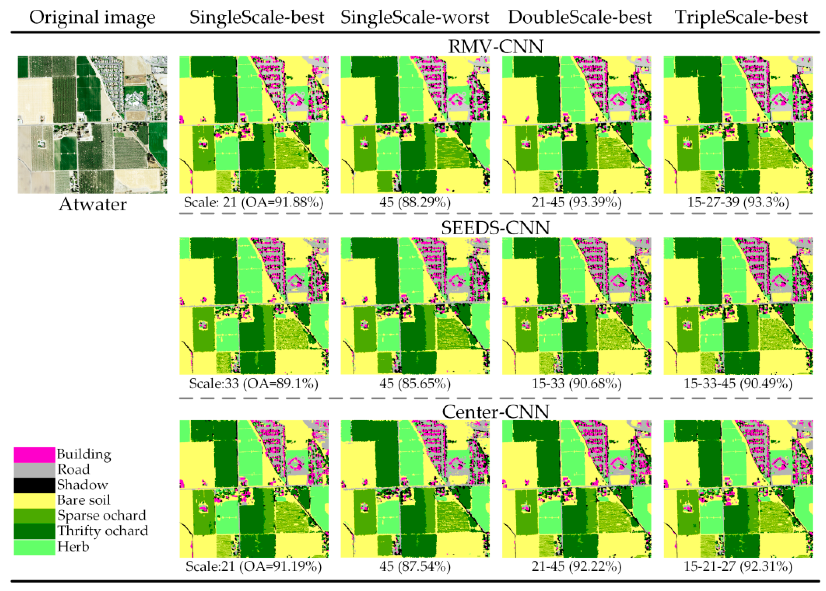
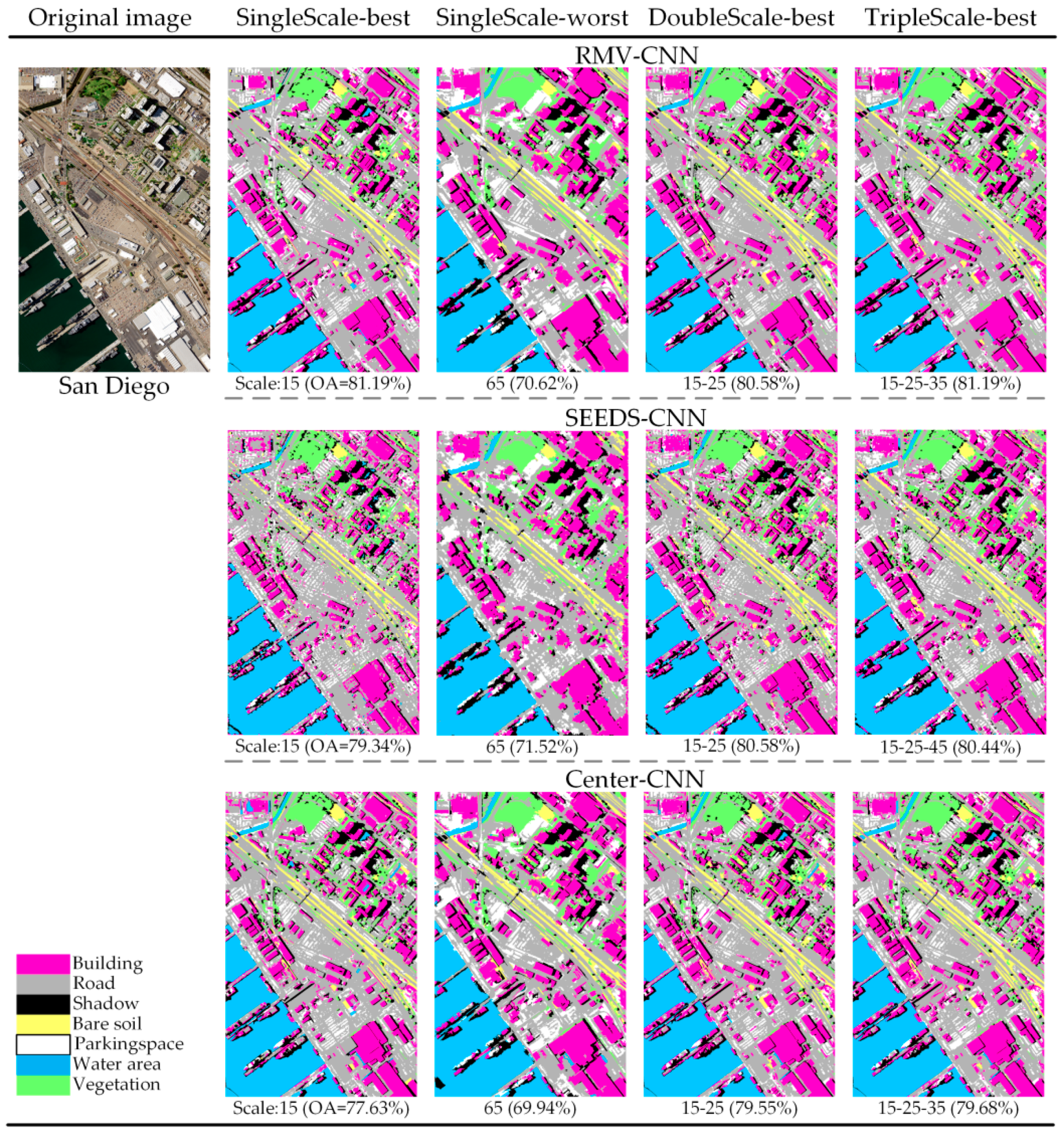
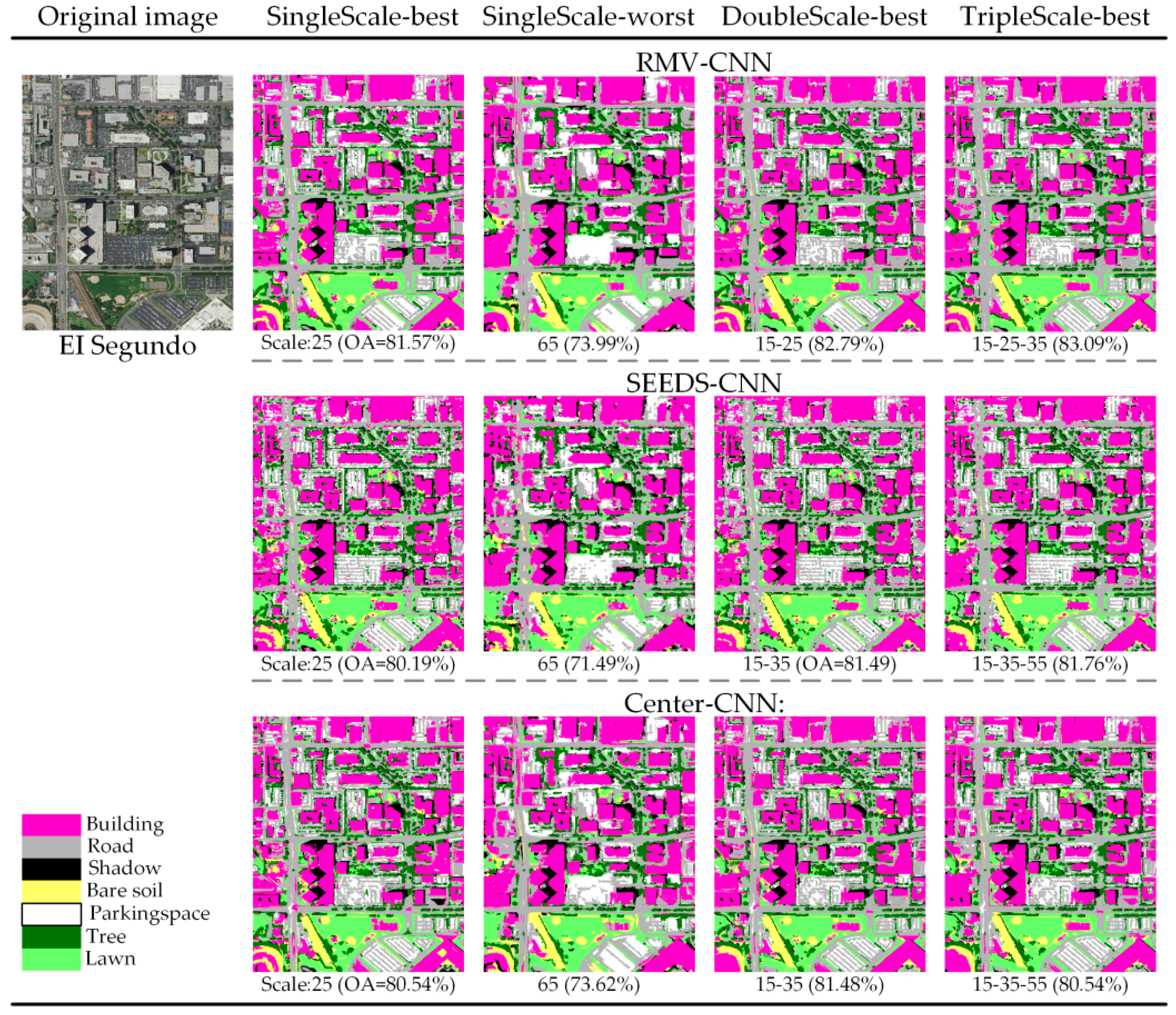
As the experiment data is too massy to show, only typical results are demonstrated here. As an example, the best and worst results at single-scales and the best results at double-scales and triple-scales are demonstrated in Figure 9, Figure 10 and Figure 11, in which the OAs (overall accuracies) for each classification are listed below the respective images.
All the final classification results using the CNN method exhibit good performance. However, there are some differences among the various CNN methods. As Figure 9, Figure 10 and Figure 11 show, the visual classification results of RMV-CNN are better than the others. The performances of SEEDS-CNN and center-CNN are comparable in the urban images, but for the agricultural image, SEEDS-CNN exhibits poor performance. The best single-scale results are all at small scales, at which the small objects such as cars and individual trees can be clearly distinguished. On the contrary, the worst single-scale results are all at large scales, at which only the buildings can be well identified. Multiple scales combining small scales and big scales perform better than single scales. The best performance at classification is at the triple-scale.
The classification accuracies of experimental images are demonstrated in Figure 12, according to which it can be seen that the proposed RMV-CNN presented the best performance of all three methods, and multiple-scales generated better classification accuracies than single-scales. For every experimental image, although all three methods had different results, the classification results still showed the same tendency at different scales, which also indicates that the selection of scale has a great impact on VHRI classification results. There are some differences between the Atwater classification results and the other two images. Obviously, RMV-CNN has a huge advantage compared to the other two methods for agricultural image classification. Also, the center-CNN also performs better than SEEDS-CNN at all scales.
For the Atwater image, as shown in Figure 12a, the three methods classification results have the same trend. The highest overall accuracy is for RMV-CNN21-45 (OA: 93.39%, kappa: 0.9144). For the single-scale, the peak of accuracy is at scale 21 (OA: 91.88%, kappa: 0.8946) and for triple-scales, the best classification result is obtained by RMV-CNN15-27-39 (OA: 93.3%, kappa: 0.8767). For SEEDS-CNN, its best performance is at scale 15-33 (OA: 90.68%, kappa: 0.8798). For center-CNN, the highest overall accuracy is at scale 15-21-27 (OA: 92.31%, kappa: 0.9006). Both of them are lower than the best performance of RMV-CNN.
As shown in Figure 12b, the EI Segundo image generated a distinguished result when the MVCCN was applied. Meanwhile, the SEEDS-CNN and center-CNN obtained the similar results. The best classification result was obtained by RMV-CNN at the triple-scale 15-25-35 (OA: 83.07%, kappa: 0.7833). For single-scale, all three methods obtained the best results at scale 25. The best result was generated by RMV-CNN25 (OA: 81.57%, kappa: 0.7656). For double-scale, the RMV-CNN still gave the best result at the scale 15-25 (OA: 82.79%, kappa: 0.7795). For triple-scales, the accuracy of RMV-CNN reached its maximum peak at triple-scale 15-25-35; while SEEDS-CNN15-35-55 (OA: 81.29%, kappa: 0.7623) generated the best result at all scales; center-CNN also obtained its finest classification result at triple-scale 15-35-55 (OA: 80.54%, kappa: 0.7509). In general, for the single-scale, all three methods showed the tendency that the classification accuracy gradually weakens from small scale to large scale; multiple-scales containing small scales showed better performance, while combined scales containing large scales were worse.
For San Diego, as shown in Figure 12c, at 18 multiple-scales, apart from scale 25-65, 15-45-65 and 25-45-65, the RMV-CNN generated better classification results than the SEEDS and the center-CNN. The best classification results of RMV-CNN appeared at single-scale 15 (OA: 81.19%, kappa: 0.7588) and triple-scale 15-25-35 (OA: 81.19%, kappa: 0.7599). For single-scales, RMV-CNN25 had the best result (OA: 81.57%, kappa: 0.7526). Moreover, small scales, e.g., scale 15, 25 and 35, performed better than large scales, such as scales 45, 55 and 65. For double-scales, all three methods gained their best results at a scale containing scale 15. For triple-scales, the best result was from RMV-CNN15-25-35 (OA: 81.19%, kappa: 0.7599). The result of SEEDS-CNN15-25-45 was slightly behind that of RMV-CNN15-25-35 (OA: 80.44%, kappa: 0.7526). The best result of center-CNN was generated at triple-scale 15-25-35 (OA: 79.68%, kappa: 0.7408). In scale combinations, double-scales and triple-scales whose basic scales included small scales performed better than those which did not. Though the accuracy of RMV-CNN was generally better than the SEEDS-CNN and the center-CNN, the accuracy was improved by only a small range. Under certain circumstances, the result of RMV-CNN was even inferior.
There are different overall accuracies at different scales for all experimental images. So, the scale effect of CNN classification is serious for VHRI classification, which will be described in Section 3.2.3.
3.2.2. Salt & Pepper Errors Caused by Scale Effect
Scale effect is an important issue in image classification [50,51]. As mentioned in Section 3.2.2, there is a serious problem of scale effect in the proposed RMV-CNN and its contrasting methods, SEEDS-CNN and center-CNN. Therefore, the scale effect has a great impact on general classification results from the macro-perspective and exists for every kind of object from the micro-perspective. The scale effect in the macro level is an accumulation of micro-level scale effects. Consequently, some interesting phenomena arose in the experimental results.
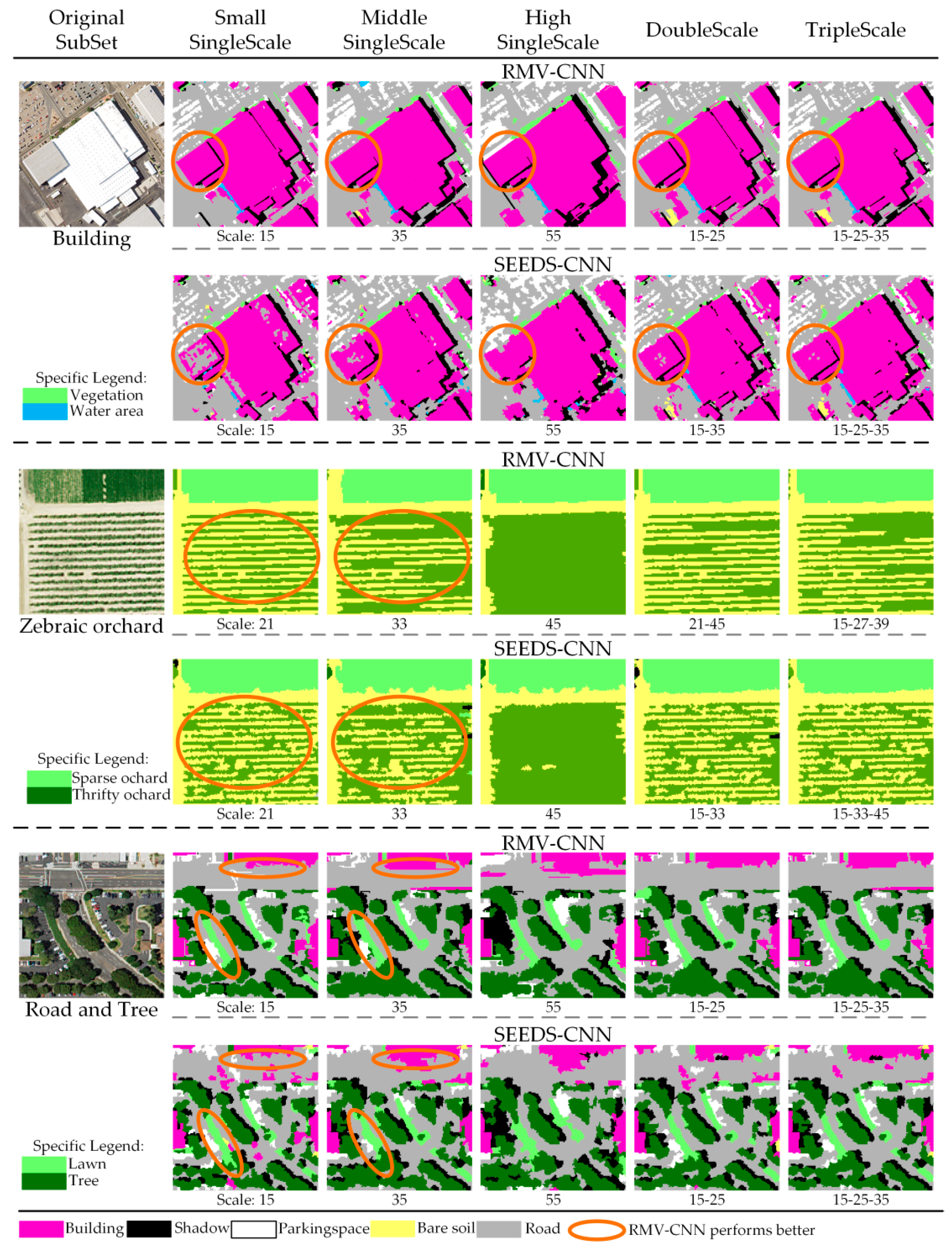
The salt and pepper errors are false classifications which sporadically appear within classification results. This phenomenon exists not only in pixel-CNN, evidently, but also in superpixel-based CNNs at the superpixel level. As shown in Figure 13, the salt and pepper errors are clearly obvious in the results of SEEDS-CNN, especially for large objects at the small single-scale. The salt and pepper errors gradually weaken and even disappear as the scale increases. However, the boundary fuzzy phenomenon subsequently arises. Objects, such as the zebraic orchard, can be clearly classified at the small scale, which is different from the salt and pepper errors. However, a serious fuzzy phenomenon happens in zebraic orchard classification at large scales or multi-scale because the zebraic orchard is only sensitive to the small scale. At large scales, boundaries between objects had lower accuracy; that is, SEEDS-CNN superpixels on boundaries were severely misclassified. Figure 13 clearly shows that classifications at large scales seemed less accurate. However, classifications of large objects barely had any salt and pepper errors at single-scales, even small scales, in RMV-CNN. In other words, the RMV-CNN can, to some extent, reduce the salt and pepper errors in classification at small scales. However, the boundary fuzzy phenomenon still remains at large scales. To emphasize the performance of RMV-CNN on solving salt and pepper error, as shown in Figure 13, using the same good boundary fitting segmentation and the same scale or scale combination, RMV-CNN classification results were compared with those from SEEDS-CNN and center-CNN.
3.2.3. Boundary Performance
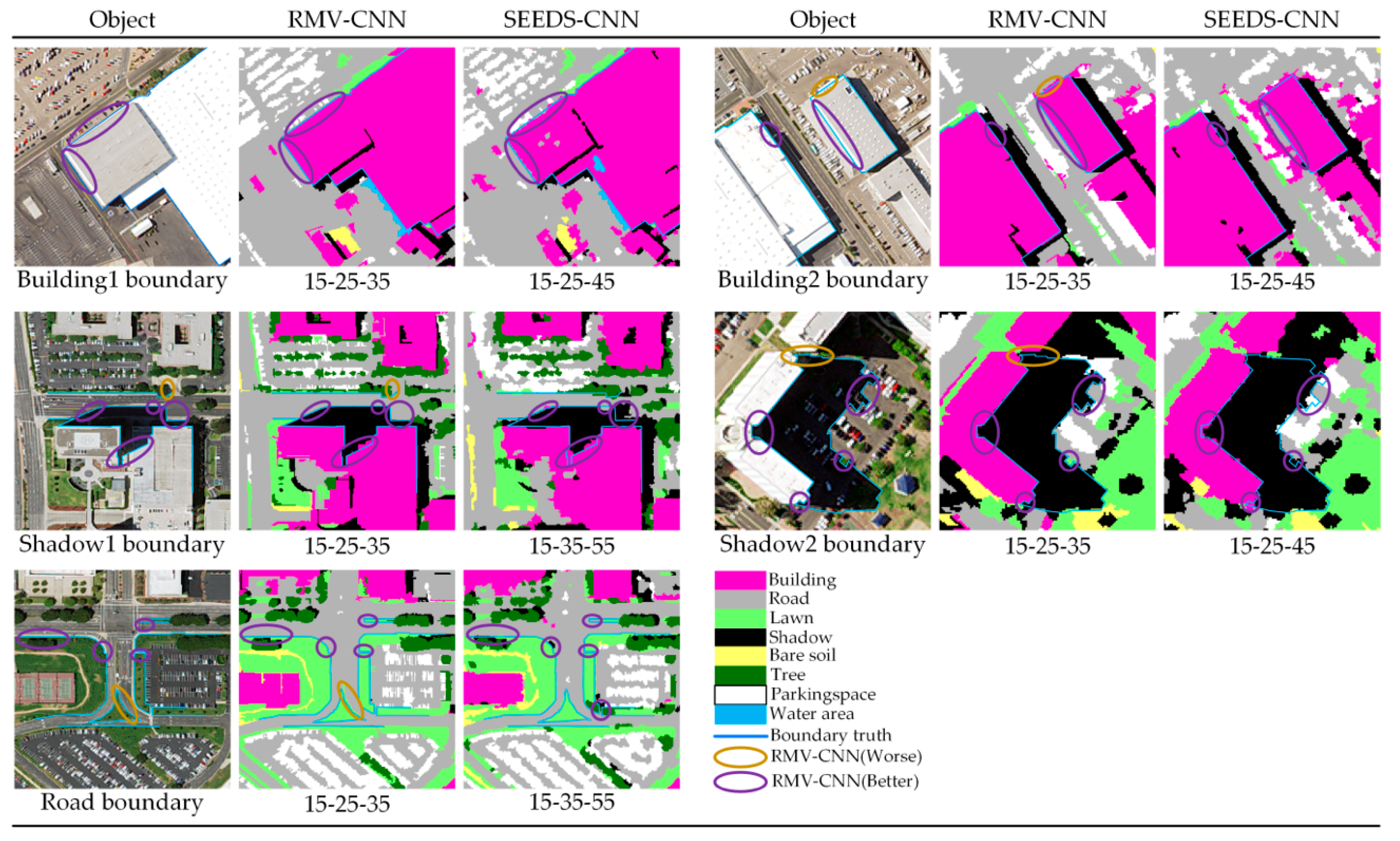
Compared with the boundary classification results of SEEDS-CNN, the results of RMV-CNN have better smoothness in the boundaries of buildings and roads, especially for curving ones. After all, the SEEDS-CNN generated the best classification result among superpixel-CNN methods and had fine boundaries; therefore, its boundary accuracy barely differs from that of the RMV-CNN. However, there is still a difference, which is reflected mainly in the boundary smoothness. Thus, it is meaningless to test boundary accuracy. Boundary performance should be shown in detail. Figure 14 demonstrates some boundary classification results at the optimal scale.
4. Discussion
Land-use classification for VHRI is complex and arduous work. Due to the intricate forms of categories, the intra-classes and the phenomenon of the same object having different spectrums abound in VHRI. The classification of VHRI needs not only to target the main categories in the image, but also to gain fine boundaries between categories. The RMV-CNN acquired favorable performance in classification due to its excellent ability to extract deep features and robustness towards complex categories.
4.1. Effectiveness of RMV-CNN for VHRI Classification
The center-CNN only considers the exclusive center point as the voter of each segmented region, while the center point voter may exist near the boundary of the object due to the complexity of the region outline shape; furthermore, because of the uncertainty of surroundings, some undesirable deep features might be involved and thus severely affect classification, leading to misclassification. However, the RMV-CNN which adds the majority voting in each region would reduce the possibility of this misclassification. An appropriate distribution of voting points is more representative of the entire region. For irregular regions, it is necessary to consider introducing more classified voting points to achieve good results.
As is known, a CNN requires the shape of all input training data to be square, thus putting strict limits on the form of input data. The square of training data is called the perceptive field from which the deep features are extracted [28]. Such superpixel segmentation results perfectly meet the requirement of perceptive field; in other words, the size of each superpixel is close to the size of receptive field. The superpixel segmentation results are propitious for center point voters to reduce the deep features that may lead to misclassifications in the process of feature extraction. In the paper [44], SEEDS has proven that it is the most suitable superpixel segmentation for CNNs, better than other commonly used superpixel segmentation methods. Therefore, for SEEDS-CNN, one voter would be sufficient. However, it is a compromise to ensure the shape of training data is suitable for the CNN, as the SEEDS-CNN emphasizes the shape compactness value in the segmentation, which might lead to the segmented region boundaries spanning different categories or being zonal. Though the SEEDS-CNN performs well in the segmentation of small objects, e.g., cars and individual trees, in the segmentation of large objects (such as the buildings) and linear objects (such as the road), the salt and pepper phenomenon and the fuzzy boundary phenomenon evidently exist. Thus, SEEDS has not only advantages but also disadvantages when combined with CNN for VHRI classification.
However, thanks to the strategy of majority voting, the proposed RMV-CNN overcomes the salt and pepper error troubles in SEEDS-CNN, especially at small scales. Furthermore, the MRS algorithm is more likely to consider a boundary item instead of the shape compactness in segmentations. It is good news for regions which have a high standard for boundary classification, e.g., buildings and roads, that the RMV-CNN emphasizes the boundary fit between categories. Therefore, basing on the good boundary fitting segmentation, the RMV-CNN generates better classification results than SEEDS-CNN; that is to say, the compactness of the segmentation result is no longer a limitation of CNNs for image classification. Any segmentation method can be applied to CNN image classification as long as there is a demand using our region-based majority voting strategy.
For some special objects, such as zebraic orchards shown in Figure 13, there is a perfect classification at small scale (scale 15) using RMV-CNN without any errors. Thus, multi-scale may not be a good selection for some special situations. However, as for the overall classification result, multi-scale is still a better option for VHRIs (Atwater’s optimal scale is 21-45, San Diego and EI Segundo’s optimal scale is 15-25-35). As an image is always more complex than a kind of object, single-scales are less eligible for such conditions because, through retraining the fully connected layer, deep features at different single-scales shall be fused and the trained CNN will be more suitable for complex images. Therefore, the obtained results by using a single scale or multi-scale are quite different.
4.2. Limitations of RMV-CNN
The CNN-based deep learning in the domain of VHRI classification has used pixel-CNN, superpixel-CNN and RMV-CNN. Not only the calculating efficiency but also the classification accuracy has gradually increased. Despite the desirable performance of RMV-CNN, it still has some defects such as the dependence on segmented results after pre-processing, as shown in Figure 15. The results need not only to ensure that small objects are clearly segmented but also to prevent large objects from being over-segmented. In fact, only by meeting the requirements above can the segmentation algorithms be used for RMV-CNN as basic segmentation. However, there is no such algorithm that perfectly meets the two requirements mentioned above.
Multi-scale is a compromise method considering overall classification. For some special situations, single scale will perform better than multi-scale. Thus, it will be a challenge in the coming research to use different locally optimal scales in different local regions.
5. Conclusions
Land-cover classification for VHRI has always been a complex and challenging task due to the complexity within categories and the complicate relations between categories in the VHRI. Traditional methods can hardly fully utilize deep features within VHRI, while the CNN overcomes this hardship and extracts deep features excellently. The proposed RMV-CNN method for VHRI classification, which is combined with the GEOBIA multiresolution segmentation and region majority voting, was firstly put forward after we thoroughly probed how to apply the CNN in the field of remote sensing.
The RMV-CNN has three merits: (1) compared with traditional methods, the RMV-CNN is able to effectively utilize the deep features in VHRI, which are the keys to VHRI classification; (2) compared with the SEEDS-CNN, the RMV-CNN can not only maintain the fine calculating efficiency, but also improve the classification accuracy and the boundary fit, and is an upgrade to the idea of superpixel-based CNN classification; and (3) compared with the center-CNN, the RMV-CNN presents a fault-tolerant advantage owing to region majority voting. It breaks through the limitations of the segmentation method. Thus, any segmentation method can be available for CNN image classification.
When it comes to the scale effect, although the RMV-CNN may, to certain extent, reduce the unreliable classification of large objects at small scales, the scale effect still evidently affects the classification results of the RMV-CNN. The selection of scale is an issue of great significance when the RMV-CNN algorithm is applied. According to the experimental results, the following points should be emphasized: (1) at least three small scales need to be introduced, and the respective deep features should be extracted to form multi-scale features; (2) the smallest scale is based on the scales of objects with the smallest sizes that are waiting to be classified; and (3) as the perceptive field of the CNN needs to learn both the inner features of the object and the features of outer surroundings, the smallest scale should not be completely based on the outline of the smallest object but should be twice its size. Then, the other two scales are determined by increasing the scale extent based on the smallest scale. Afterwards, the VHRI would be classified by the RMV-CNN at triple-scales.
Additionally, there are still some issues that should be further focused on. The performance of RMV-CNN classification is very dependent on segmentation, and a segmentation method that can generate accurate boundaries is the key to RMV-CNN. Also, applications of the CNN in remote sensing are limited to raster images, which are essentially a series of matrix operation. However, in such an information-abundant era, different types of data, including vector data and some social sensing data, emerge in an endless stream, which provides another supplement for geosciences. Research in remote sensing should not consider only a single type of data but needs to introduce multiple source data and make full use of its advantages. Though the CNN is able to extract objects’ deep features and perceive the background information of certain objects, it still fails to learn the deep topological relations between objects. Topological relation learning will be the research priority of deep learning-based remote sensing image understanding in the coming years.
Author Contributions
Conceptualization, X.L. and D.M.; methodology, X.L.; software, X.L., T.L. and K.Z.; validation, X.L., D.M. and T.L.; formal analysis, X.L., D.M.; resources, X.L.; data curation, X.L., T.L., K.Z., M.W. and H.B.; writing—original draft preparation, X.L.; writing—review and editing, X.L., D.M. and K.Z.; supervision, D.M.; project administration, D.M.; funding acquisition, D.M.
Funding
This research was supported by the National Key Research and Development Program (2017YFB0503600), the National Natural Science Foundation of China (41671369, 41671341), and the Fundamental Research Funds for the Central Universities.
Conflicts of Interest
The authors declare no conflict of interest.
References
- Ibarrolaulzurrun, E.; Marcello, J.; Gonzalomartin, C. Advanced Classification of Remote Sensing High Resolution Imagery. An Application for the Management of Natural Resources; Springer: Cham, Switzerland, 2018. [Google Scholar]
- Machín, A.M.; Marcello, J.; Cordero, A.I.H.; Eugenio, F. Vegetation species mapping in a coastal-dune ecosystem using high resolution satellite imagery. GISci. Remote Sens. 2018. [Google Scholar] [CrossRef]
- Marcello, J.; Eugenio, F.; Marques, F.; Martín, J. Precise classification of coastal benthic habitats using high resolution Worldview-2 imagery. In Proceedings of the Geoscience and Remote Sensing Symposium, Milan, Italy, 26–31 July 2015; pp. 2307–2310. [Google Scholar]
- Tao, J.; Shu, N.; Wang, Y.; Hu, Q.; Zhang, Y. A study of a Gaussian mixture model for urban land-cover mapping based on VHR remote sensing imagery. Int. J. Remote Sens. 2016, 37, 1–13. [Google Scholar] [CrossRef]
- Blaschke, T. Object based image analysis for remote sensing. ISPRS J. Photogramm. Remote Sens. 2010, 65, 2–16. [Google Scholar] [CrossRef]
- Blaschke, T.; Hay, G.J.; Kelly, M.; Lang, S.; Hofmann, P.; Addink, E.; Feitosa, R.Q.; Van der Meer, F.; Van der Werff, H.; Van Coillie, F.; et al. Geographic Object-Based Image Analysis—Towards a new paradigm. ISPRS J. Photogramm. Remote Sens. 2014, 87, 180–191. [Google Scholar] [CrossRef] [PubMed]
- Mondini, A.C.; Marchesini, I.; Rossi, M.; Chang, K.T.; Pasquariello, G.; Guzzetti, F. Bayesian framework for mapping and classifying shallow landslides exploiting remote sensing and topographic data. Geomorphology 2013, 201, 135–147. [Google Scholar] [CrossRef]
- Ouyang, Y.; Ma, J.; Dai, Q. Bayesian Multi-net Classifier for classification of remote sensing data. Int. J. Remote Sens. 2006, 27, 4943–4961. [Google Scholar] [CrossRef]
- He, C.; Liu, X.; Feng, D.; Shi, B.; Luo, B.; Liao, M. Hierarchical Terrain Classification Based on Multilayer Bayesian Network and Conditional Random Field. Remote Sens. 2017, 9, 96. [Google Scholar] [CrossRef]
- Berthod, M.; Kato, Z.; Yu, S.; Zerubia, J. Bayesian Image Classification Using Markov Random Fields. Image Vis. Comput. 1996, 14, 285–295. [Google Scholar] [CrossRef]
- Thomaz, C.E.; Gillies, D.F.; Feitosa, R.Q. A New Covariance Estimate for Bayesian Classifiers in Biometric Recognition. IEEE Trans. Circuit Syst. Video Technol. 2004, 14, 214–223. [Google Scholar] [CrossRef]
- Segata, N.; Pasolli, E.; Melgani, F.; Blanzieri, E. Local SVM approaches for fast and accurate classification of remote-sensing images. Int. J. Remote Sens. 2012, 33, 6186–6201. [Google Scholar] [CrossRef]
- Zhou, J.; Qin, J.; Gao, K.; Leng, H. SVM-based soft classification of urban tree species using very high-spatial resolution remote-sensing imagery. Int. J. Remote Sens. 2016, 37, 2541–2559. [Google Scholar] [CrossRef]
- Negri, R.G.; Dutra, L.V.; Sant’Anna, S.J.S. An innovative support vector machine based method for contextual image classification. ISPRS J. Photogramm. Remote Sens. 2014, 87, 241–248. [Google Scholar] [CrossRef]
- Negri, R.G.; Sant’Anna, S.J.S.; Dutra, L.V. A new contextual version of Support Vector Machine based on hyperplane translation. In Proceedings of the 2013 IEEE International Geoscience and Remote Sensing Symposium, Melbourne, VIC, Australia, 21–26 July 2013; pp. 3116–3119. [Google Scholar]
- Zhou, W.; Ming, D.; Xu, L.; Bao, H.; Wang, M. Stratified Object-Oriented Image Classification Based on Remote Sensing Image Scene Division. J. Spectrosc. 2018. [Google Scholar] [CrossRef]
- Negri, R.G.; Dutra, L.V.; Freitas, C.D.C.; Lu, D. Exploring the Capability of ALOS PALSAR L-Band Fully Polarimetric Data for Land Cover Classification in Tropical Environments. IEEE J. Sel. Top. Appl. Earth Obs. Remote Sens. 2016, 9, 5369–5384. [Google Scholar] [CrossRef]
- Negri, R.G.; Silva, E.A.D.; Casaca, W. Inducing Contextual Classifications With Kernel Functions Into Support Vector Machines. IEEE Geosci. Remote Sens. Lett. 2018, 15, 962–966. [Google Scholar] [CrossRef]
- Wu, S.-S.; Qiu, X.; Usery, E.L.; Wang, L. Using Geometrical, Textural, and Contextual Information of Land Parcels for Classification of Detailed Urban Land Use. Ann. Assoc. Am. Geogr. 2009, 99, 76–98. [Google Scholar] [CrossRef]
- Zhao, W.; Guo, Z.; Yue, J.; Luo, L.; Luo, L. On combining multiscale deep learning features for the classification of hyperspectral remote sensing imagery. Int. J. Remote Sens. 2015, 36, 3368–3379. [Google Scholar] [CrossRef]
- Lecun, Y.; Bengio, Y.; Hinton, G. Deep learning. Nature 2015, 521, 436. [Google Scholar] [CrossRef]
- Luus, F.P.S.; Salmon, B.P.; Bergh, F.V.D.; Maharaj, B.T.J. Multiview Deep Learning for Land-Use Classification. IEEE Geosci. Remote Sens. Lett. 2015, 12, 2448–2452. [Google Scholar] [CrossRef] [Green Version]
- Cheng, G.; Wang, Y.; Xu, S.; Wang, H.; Xiang, S.; Pan, C. Automatic Road Detection and Centerline Extraction via Cascaded End-to-End Convolutional Neural Network. IEEE Trans. Geosci. Remote Sens. 2017, 55, 3322–3337. [Google Scholar] [CrossRef]
- Hu, F.; Xia, G.S.; Hu, J.; Zhang, L. Transferring Deep Convolutional Neural Networks for the Scene Classification of High-Resolution Remote Sensing Imagery. Remote Sens. 2015, 7, 14680–14707. [Google Scholar] [CrossRef] [Green Version]
- Othman, E.; Bazi, Y.; Alajlan, N.; Alhichri, H.; Melgani, F. Using convolutional features and a sparse autoencoder for land-use scene classification. Int. J. Remote Sens. 2016, 37, 2149–2167. [Google Scholar] [CrossRef]
- Dong, Z.; Pei, M.; He, Y.; Liu, T.; Dong, Y.; Jia, Y. Vehicle Type Classification Using Unsupervised Convolutional Neural Network. In Proceedings of the International Conference on Pattern Recognition, Stockholm, Sweden, 6 March 2015; pp. 172–177. [Google Scholar]
- Gallego, A.J.; Pertusa, A.; Gil, P. Automatic Ship Classification from Optical Aerial Images with Convolutional Neural Networks. Remote Sens. 2018, 10, 511. [Google Scholar] [CrossRef]
- Chen, Y.; Jiang, H.; Li, C.; Jia, X.; Ghamisi, P. Deep Feature Extraction and Classification of Hyperspectral Images Based on Convolutional Neural Networks. IEEE Trans. Geosci. Remote Sens. 2016, 54, 6232–6251. [Google Scholar] [CrossRef]
- Qi, K.; Guan, Q.; Yang, C.; Peng, F.; Shen, S.; Wu, H. Concentric Circle Pooling in Deep Convolutional Networks for Remote Sensing Scene Classification. Remote Sens. 2018, 10, 934. [Google Scholar] [CrossRef]
- Li, P.; Ren, P.; Zhang, X.; Wang, Q.; Zhu, X.; Wang, L. Region-Wise Deep Feature Representation for Remote Sensing Images. Remote Sens. 2018, 10, 871. [Google Scholar] [CrossRef]
- Maggiori, E.; Tarabalka, Y.; Charpiat, G.; Alliez, P. Convolutional Neural Networks for Large-Scale Remote-Sensing Image Classification. IEEE Trans. Geosci. Remote Sens. 2016, 55, 645–657. [Google Scholar] [CrossRef]
- Ming, D.; Zhou, T.; Wang, M.; Tan, T. Land cover classification using random forest with genetic algorithm-based parameter optimization. J. Appl. Remote Sens. 2016, 10, 035021. [Google Scholar] [CrossRef]
- Zhang, C.; Sargent, I.; Pan, X.; Gardiner, A.; Hare, J.; Atkinson, P.M. VPRS-Based Regional Decision Fusion of CNN and MRF Classifications for Very Fine Resolution Remotely Sensed Images. IEEE Trans. Geosci. Remote Sens. 2018, 56, 4507–4521. [Google Scholar] [CrossRef] [Green Version]
- Zhang, C.; Pan, X.; Li, H.; Gardiner, A.; Sargent, I.; Hare, J.; Atkinson, P.M. A hybrid MLP-CNN classifier for very fine resolution remotely sensed image classification. ISPRS J. Photogramm. Remote Sens. 2017, 140, 133–144. [Google Scholar] [CrossRef]
- Zhao, W.; Jiao, L.; Ma, W.; Zhao, J.; Zhao, J.; Liu, H.; Cao, X.; Yang, S. Superpixel-Based Multiple Local CNN for Panchromatic and Multispectral Image Classification. IEEE Trans. Geosci. Remote Sens. 2017, 55, 4141–4156. [Google Scholar] [CrossRef]
- Gonzalo-Martin, C.; Garcia-Pedrero, A.; Lillo-Saavedra, M.; Menasalvas, E. Deep learning for superpixel-based classification of remote sensing images. In Proceedings of the GEOBIA 2016: Solutions and Synergies, Enschede, The Netherlands, 14–16 September 2016. [Google Scholar]
- Cao, J.; Chen, Z.; Wang, B. Deep Convolutional networks with superpixel segmentation for hyperspectral image classification. In Proceedings of the Geoscience and Remote Sensing Symposium, Beijing, China, 10–15 July 2016; pp. 3310–3313. [Google Scholar]
- Wang, S.; Lu, H.; Yang, F.; Yang, M.H. Superpixel tracking. In Proceedings of the International Conference on Computer Vision, Barcelona, Spain, 6–13 November 2011; pp. 1323–1330. [Google Scholar]
- Liu, M.Y.; Tuzel, O.; Ramalingam, S.; Chellappa, R. Entropy rate superpixel segmentation. In Proceedings of the Computer Vision and Pattern Recognition, Colorado Springs, CO, USA, 20–25 June 2011; pp. 2097–2104. [Google Scholar]
- Csillik, O. Fast Segmentation and Classification of Very High Resolution Remote Sensing Data Using SLIC Superpixels. Remote Sens. 2017, 9, 243. [Google Scholar] [CrossRef]
- Happ, P.N.; Bentes, C.; Feitosa, R.Q.; Ferreira, R.D.S.; Farias, R. A Cloud Computing Strategy for Region-Growing Segmentation. IEEE J. Sel. Top. Appl. Earth Obs. Remote Sens. 2016, 9, 5294–5303. [Google Scholar] [CrossRef]
- Zhao, W.; Du, S. Learning multiscale and deep representations for classifying remotely sensed imagery. ISPRS J. Photogramm. Remote Sens. 2016, 113, 155–165. [Google Scholar] [CrossRef]
- Wang, M.; Liu, X.; Gao, Y.; Ma, X.; Soomro, N.Q. Superpixel segmentation: A benchmark. Signal Process. Image Commun. 2017, 56, 28–39. [Google Scholar] [CrossRef]
- Lv, X.; Ming, D.; Chen, Y.; Wang, M. Very High Resolution Remote Sensing Image Classification with SEEDS-CNN and Scale Effect Analysis for Superpixel CNN Classification. Int. J. Remote Sens. 2018. [Google Scholar] [CrossRef]
- Rabiee, H.R.; Kashyap, R.; Safavian, S.R. Multiresolution segmentation-based image coding with hierarchical data structures. In Proceedings of the 1996 IEEE International Conference on Acoustics, Speech, and Signal, Atlanta, GA, USA, 9 May 1996; pp. 1870–1873. [Google Scholar]
- Comaniciu, D.; Meer, P. Mean Shift: A Robust Approach Toward Feature Space Analysis. IEEE Trans. Pattern Anal. Mach. Intell. 2002, 24, 603–619. [Google Scholar] [CrossRef]
- Zhang, C.; Sargent, I.; Pan, X.; Li, H.; Gardiner, A.; Hare, J. An object-based convolutional neural network (OCNN) for urban land use classification. Remote Sens. Environ. 2018, 216, 57–70. [Google Scholar] [CrossRef]
- Krizhevsky, A.; Sutskever, I.; Hinton, G.E. ImageNet classification with deep convolutional neural networks. In Proceedings of the International Conference on Neural Information Processing Systems, New York, NY, USA, 3–8 December 2012; pp. 1097–1105. [Google Scholar]
- Chavez, P.S. Statistical method for selecting LANDSAT MSS ratios. J. Appl. Photogr. Eng. 1982, 8, 23–30. [Google Scholar]
- Ming, D.; Li, J.; Wang, J.; Zhang, M. Scale parameter selection by spatial statistics for GeOBIA: Using mean-shift based multi-scale segmentation as an example. ISPRS J. Photogramm. Remote Sens. 2015, 106, 28–41. [Google Scholar] [CrossRef]
- Ming, D.; Yang, J.; Li, L.; Song, Z. Modified ALV for selecting the optimal spatial resolution and its scale effect on image classification accuracy. Math. Comput. Model. 2011, 54, 1061–1068. [Google Scholar] [CrossRef]
Figure 1.
Workflow of the region-based majority voting convolutional neural network (RMV-CNN).

Figure 2.
The network structure of AlexNet. Conv: convolutional layer; Pool: pooling layer; FC: fully-connected layer. The number below the figure is the dimension of the data.
Figure 2.
The network structure of AlexNet. Conv: convolutional layer; Pool: pooling layer; FC: fully-connected layer. The number below the figure is the dimension of the data.

Figure 3.
Random points generation workflow. K: the number of required points; Num: the number of points currently generated.
Figure 3.
Random points generation workflow. K: the number of required points; Num: the number of points currently generated.

Figure 4.
The process of region majority voting.

Figure 5.
Experimental images: (a) the Atwater image; (b) the EI Segundo image; (c) the San Diego image.
Figure 5.
Experimental images: (a) the Atwater image; (b) the EI Segundo image; (c) the San Diego image.

Figure 6.
Samples of the three experimental images. (a) Atwater; (b) EI Segundo; (c) San Diego.

Figure 7.
The local results of multiresolution segmentation (MRS) and superpixels extracted via energy-driven sampling (SEEDS) segmentation.
Figure 7.
The local results of multiresolution segmentation (MRS) and superpixels extracted via energy-driven sampling (SEEDS) segmentation.


Figure 8.
The accuracy assessment points of each image. (a) Atwater; (b) EI Segundo; (c) San Diego.

Figure 9.
The classification result of the Atwater image at different scales.

Figure 10.
The classification result of the San Diego image at different scales.

Figure 11.
The classification result of the El Segundo image at different scales.

Figure 12.
Classification overall accuracy results. (a) Atwater; (b) EI Segundo; (c) San Diego.

Figure 13.
The salt and pepper errors of three sub-datasets classifications at some scales.

Figure 14.
The comparison of RMV-CNN and SEEDS-CNN boundary performance at their optimal scale combinations.
Figure 14.
The comparison of RMV-CNN and SEEDS-CNN boundary performance at their optimal scale combinations.

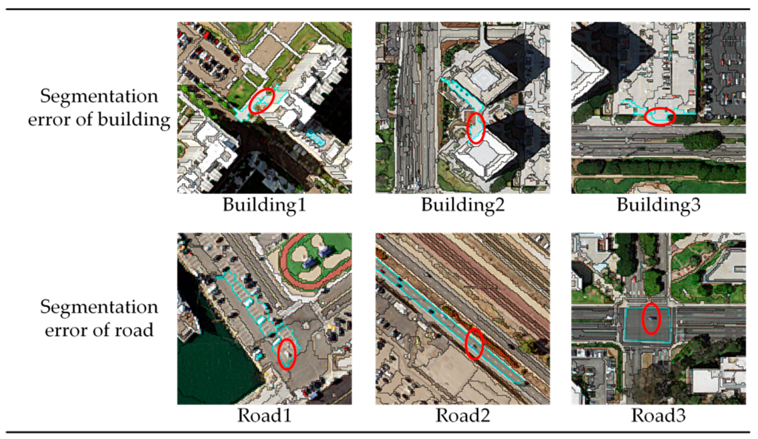
Figure 15.
Some errors of the multiresolution segmentation of images. The red circle indicates the error object in the segmentation region.
Figure 15.
Some errors of the multiresolution segmentation of images. The red circle indicates the error object in the segmentation region.


Table 1.
Detailed information about the three images. OIF: optimal index factor. R: red; G: green; B: blue; NIR: near infrared.
Table 1.
Detailed information about the three images. OIF: optimal index factor. R: red; G: green; B: blue; NIR: near infrared.
| Image | Size (m2) | Location | Spatial Resolution | Band Combination | OIF Value | Main Categories |
|---|---|---|---|---|---|---|
| Atwater | 1300 × 1200 | 120°37′30″W 37°20′30″N | 1 m | R, G, B R, G, NIR R, B, NIR G, B, NIR | 45.95 82.82 95.40 85.52 | Building Road Bare soil Shadow Sparse orchard Thrifty orchard Herb |
| San Diego | 1120 × 1740 | 117°7′30″W 32°41′0″N | 1 m | R, G, B R, G, NIR R, B, NIR G, B, NIR | 52.61 63.50 64.39 61.19 | Building Parking space road Bare soil Shadow vegetation Water area |
| EI Segundo | 950 × 1150 | 118°23′45″W 33°55′0″ | 1 m | R, G, B R, G, NIR R, B, NIR G, B, NIR | 56.48 83.19 91.73 86.78 | Building Parking space Road Bare soil Shadow Lawn Tree |
Table 2.
The training and validation volumes of each image.
| Data | Categories | ||||||
|---|---|---|---|---|---|---|---|
| Atwater | Building | Bare soil | Road | Shadow | Sparse orchard | Thrifty orchard | Herb |
| Training | 90 | 320 | 198 | 83 | 192 | 301 | 256 |
| Validation | 22 | 80 | 50 | 21 | 48 | 75 | 64 |
| EI Segundo | Building | Bare soil | Road | Shadow | Parking space | Tree | Lawn |
| Training | 1760 | 180 | 840 | 360 | 440 | 480 | 380 |
| Validation | 440 | 45 | 210 | 90 | 110 | 120 | 95 |
| San Diego | Building | Bare soil | Road | Shadow | Parking space | Vegeta-tion | Water |
| Training | 1408 | 384 | 1568 | 768 | 716 | 640 | 480 |
| Validation | 352 | 96 | 392 | 192 | 179 | 160 | 120 |
© 2018 by the authors. Licensee MDPI, Basel, Switzerland. This article is an open access article distributed under the terms and conditions of the Creative Commons Attribution (CC BY) license (http://creativecommons.org/licenses/by/4.0/).
Share and Cite
MDPI and ACS Style
Lv, X.; Ming, D.; Lu, T.; Zhou, K.; Wang, M.; Bao, H. A New Method for Region-Based Majority Voting CNNs for Very High Resolution Image Classification. Remote Sens. 2018, 10, 1946. https://doi.org/10.3390/rs10121946
AMA Style
Lv X, Ming D, Lu T, Zhou K, Wang M, Bao H. A New Method for Region-Based Majority Voting CNNs for Very High Resolution Image Classification. Remote Sensing. 2018; 10(12):1946. https://doi.org/10.3390/rs10121946
Chicago/Turabian StyleLv, Xianwei, Dongping Ming, Tingting Lu, Keqi Zhou, Min Wang, and Hanqing Bao. 2018. "A New Method for Region-Based Majority Voting CNNs for Very High Resolution Image Classification" Remote Sensing 10, no. 12: 1946. https://doi.org/10.3390/rs10121946
Note that from the first issue of 2016, this journal uses article numbers instead of page numbers. See further details here.