Article

Evaluating the Temporal Dynamics of Uncertainty Contribution from Satellite Precipitation Input in Rainfall-Runoff Modeling Using the Variance Decomposition Method

1
State Key Laboratory of Water Resources and Hydropower Engineering Science, Wuhan University, Wuhan 430072, China
2
Department of Geosciences, University of Oslo, P.O. Box 1022 Blindern, N-0315 Oslo, Norway
*
Author to whom correspondence should be addressed.
Remote Sens. 2018, 10(12), 1876; https://doi.org/10.3390/rs10121876
Submission received: 8 October 2018 / Revised: 19 November 2018 / Accepted: 20 November 2018 / Published: 23 November 2018
(This article belongs to the Section Remote Sensing in Geology, Geomorphology and Hydrology)

Abstract

:
Satellite precipitation estimates (SPE), characterized by high spatial-temporal resolution, have been increasingly applied to hydrological modeling. However, the errors and bias inherent in SPE are broadly recognized. Yet, it remains unclear to what extent input uncertainty in hydrological models driven by SPE contributes to the total prediction uncertainty, resulting from difficulties in uncertainty partitioning. This study comprehensively quantified the input uncertainty contribution of three precipitation inputs (Tropical Rainfall Measurement Mission (TRMM) near-real-time 3B42RTv7 product, TRMM post-real-time 3B42v7 product and gauge-based precipitation) in rainfall-runoff simulation, using two hydrological models, the lumped daily Ge´nie Rural (GR) and distributed Coupled Routing and Excess STorage (CREST) models. For this purpose, the variance decomposition method was applied to disaggregate the total streamflow modeling uncertainty into seven components (uncertainties in model input, parameter, structure and their three first-order interaction effects, and residual error). The results showed that the total uncertainty in GR was lowest, moderate and highest when forced by gauge precipitation, 3B42v7 and 3B42RTv7, respectively. While the total uncertainty in CREST driven by 3B42v7 was lowest among the three input data sources. These results highlighted the superiority of post-real-time 3B42v7 in hydrological modeling as compared to real-time 3B42RTv7. All the input uncertainties in CREST driven by 3B42v7, 3B42RTv7 and gauge-based precipitation were lower than those in GR correspondingly. In addition, the input uncertainty was lowest in 3B42v7-driven CREST model while highest in gauge precipitation-driven GR model among the six combination schemes (two models combined with three precipitation inputs abovementioned). The distributed CREST model was capable of making better use of the spatial distribution advantage of SPE especially for the TRMM post-real-time 3B42v7 product. This study provided new insights into the SPE’s hydrological utility in the context of uncertainty, being significant for improving the suitability and adequacy of SPE to hydrological application.

Graphical Abstract

1. Introduction

Precipitation is one of most critical input variables for accurate hydrological simulation [1,2]. Studies on the precipitation input impacts on the performance of hydrological models are fewer, compared to the attention paid to sophisticated rainfall-runoff modeling approaches [3]. Concretely, for example, traditional attention towards hydrological model uncertainty was mostly paid on parameter uncertainty and/or structure uncertainty inherent in models per se. Recently, input data uncertainty related to the external forcing has been regarded as a source of systematic bias in rainfall-runoff process with its increasingly pervasive influence on hydrological models [4,5,6].
Satellite precipitation estimates (SPE) are promising alternatives to precipitation measurement in hydrological utility, particularly over the gauge-sparse or ungauged regions [7,8,9,10,11]. Although SPE are capable of reproducing spatial-temporal precipitation at high resolutions, the accuracy in supporting reliable hydrological modeling is limited [12,13]. This is primarily because of the indirect observation and noisy retrieval of such high-resolution satellite precipitation [14] and resampling errors from coarse to fine resolution in hydrological utility [15]. Taking the Tropical Rainfall Measurement Mission (TRMM) Multi-satellite Precipitation Analysis (TMPA) products as an example, Maggioni et al. [16] analyzed TRMM Version-7 near-real-time (hereafter referred as 3B42RTv7) and post-real-time (referred as 3B42v7) products over the United States. It was concluded that the random error is the main error component of TRMM precipitation which is larger than systematic error, and both of these errors strongly depended on satellite rain rates. Yong et al. [17] reported that the error components of the TRMM estimates showed strong seasonal and regional differences over mainland China. Maggioni et al. [18] further stated that the uncertainty of 3B42RTv7 was higher during the warm season characterized by convective storms, relative to the cold season with organized stratiform precipitation. Therefore, SPE with random errors and biases could induce input uncertainty in streamflow and flood simulation, resulting in unreliable decision making or guidance in engineering and policy.
Several attempts have been made to identify the input uncertainty induced by SPE in hydrological modeling. Knoche et al. [12] jointly analyzed the modeling uncertainty which resulted from various satellite-based forcing data and hydrological models. Shah and Mishra [19] estimated the streamflow monitoring uncertainty (characterized by standard deviation) originating from the biased SPE-induced initial conditions. Despite these single-source uncertainty analyses, however, the input uncertainty in hydrological models driven by SPE and its interaction with other uncertainty sources, such as parameter and model structure uncertainty, still remain unclear, mainly due to difficulties in uncertainty component partitioning.
One way to obtain input uncertainty in multi-source uncertainty context is to drive a hydrologic model with multiple rainfall input series or hypothetical forcing data chains [20,21]. Hierarchical Bayesian framework was introduced to quantify uncertainty in rainfall using latent variables (e.g., rainfall multipliers), and then various later studies in surface hydrology have investigated the role of input data in prediction uncertainty on this base [22]. Within this framework, Kavetski et al. [23] established the Bayesian total error analysis (BATEA) method to explicitly account for input uncertainty in hydrological modeling. Ajami et al. [24] developed an integrated Bayesian uncertainty estimator (IBUNE) to represent input, parameter and model structure uncertainties. Nevertheless, this Bayesian paradigm accounts for input uncertainty in a stochastically optimal process, which may depend on conditioning values.
More recently, variance-based methods circumvent the above downside of Bayesian through a holistic consideration of completely partitioning multi-source uncertainties [6]. Related work has aimed at identifying the respective contributions of input, parameter and structure uncertainties to the total uncertainty, which can be conductive to detect main contributors of multiple potential uncertainties and to indicate model deficiencies. More importantly, it has the potential to explicitly reveal the insight of the interaction effect of individual uncertainty sources, as the interactions may account for a non-negligible part of the total uncertainty but they are hard to diagnose [6]. To statistically achieve a robust disaggregating technique using a variance-based method, the practical challenges remain in the configuration of model setup to ensure available comparability of the different terms, and the definition of decomposed factors to facilitate well-posed inference. For example, Addor et al. [25] decomposed the uncertainty arising from different sources of emission scenarios, climate models, their post-processing, hydrological models, and natural variability in the ensemble of streamflow projections using analyses of variance. The choice of emission scenarios (input forcing) played a large role by the end of the 21st century. Mockler et al. [6] introduced a similar approach to identify rainfall and parameter uncertainties in streamflow predictions and concluded that rainfall input was the leading source of total uncertainty. These studies quantified the input uncertainty in hydrological modeling under a more holistic conceptual framework of uncertainty, compared to the Bayesian framework. In circumstances where the initial SPE products could be biased and associated input uncertainties have not been quantified well, it is more desirable to infer the level of input uncertainty and the relative importance to total prediction uncertainty in hydrological modeling. Hence, studies are needed to better understand the impacts of SPE input uncertainty on hydrological prediction. However, the variance decomposition method has rarely been introduced into identifying the multi-source uncertainties involved in SPE-induced input uncertainty and its interaction effect with others in hydrological models.
The aims of this paper are twofold: (1) Exploring how the time sequential magnitude and relative contribution of precipitation (two SPE products vs. gauge reference) input uncertainty and its interactions with other uncertainties (i.e., the parameter and model structure uncertainty) in streamflow simulations can be quantified using a variance-based method, and (2) identifying what impact three precipitation input scenarios combined with two hydrological models exerted on the input uncertainty. As for the two models, the suite of daily GR (Ge´nie Rural) hydrological modeling tools developed by the Hydrology Research Group of Irstea institute in France including GR4J, GR5J and GR6J and the Coupled Routing and Excess STorage (CREST) hydrologic model were applied as lumped and distributed models respectively. Specifically, the remaining part of this paper is organized as follows. Section 2 below describes the study area and data used. Section 3 presents a parsimonious framework of the model configuration coupling multiple precipitation forcing with parameter sets and model structures. Section 4 provides and discusses the results. Section 5 concludes the study.

2. Study Area and Data

2.1. Ganjiang River Basin

The Ganjiang River is the seventh largest tributary of the Yangtze River, located between 24°22.8′–28°48′ N and 113°33.6′–116°43.2′ E in the Jiangxi province of southeast China. In the 81,020 km2 draining area, the terrain is complex with mountains (43.9%) in the headwater area, low hills (<200 m, 31.5%) in the central part of the basin and alluvial plains (24.6%) in the lower reach, where the elevation (11–1950 m) roughly decreases from south to north. The area has a typical subtropical monsoon climate with an annual mean air temperature of approximately 18.75 °C and annual mean rainfall of 1400 to 1600 mm. Over 62.29% of the total rainfall is concentrated in the period from April to August. In addition to the heterogeneity of rainfall in seasons, the spatial distribution of rainfall is also non-uniform. There is abundant rain falling in the eastern part and northwestern part of the basin (above 1723.9 mm annually on average) and less rainfall in the central part and the lower reach (below 1368.02 mm annually on average). Moreover, actual evapotranspiration usually exceeds rainfall between July and October, producing drought regionally.

2.2. Precipitation Datasets

Specifically, Figure 1 shows the spatial distribution of rain gauges used for comparison as well as the pan evaporation and discharge stations. The daily precipitation and pan evaporation across Ganjiang River basin, and streamflow data at the Waizhou station, provided by hydrological bureau of Jiangxi province, were collected during the period 2000–2013. Several nearby stations outside the basin were also used to calculate the basin-wide precipitation and potential evapotranspiration (see Figure 1). Precipitation is the main driver in rainfall-runoff modeling. The pan evaporation is used to calculate how much effective precipitation left in the runoff generation, as the evapotranspiration process is a critical hydrophysical process in hydrological models. The observed streamflow data provide a benchmark in model calibration and uncertainty analysis. To ensure the accuracy of observation values, outlier processing, spatial consistency diagnosing and internal consistency checking served as the quality control procedure following Ren et al. [26]. The daily ground rainfall and pan evaporation data were interpolated into gridded datasets with 0.02° × 0.02° spatial resolution using the Inverse Distance Weighted Interpolation method. This interpolated network data was used to drive the distributed hydrological CREST model, and the average of all interpolated grids was taken as areal average precipitation or pan evaporation to input the lumped GR model. The average of all interpolated grids used here aimed to reduce the uneven density of rain gauges. The TRMM SPE data, introduced below, also adopted the 0.02° × 0.02° grid network and average of these grids as inputs of CREST and GR respectively. In this study, when referring to the ground-based gridded precipitation using interpolation technique, “Gauge” precipitation was used for simplification.
The TMPA estimates were derived first by calibrating and combining microwave precipitation (MW), then creating infrared precipitation (IR) estimates using the calibrated MW, and lastly merging the MW and IR estimates [27,28]. Briefly, the production of TMPA estimates depends on two input sets of passive MW and IR sensors. The passive MW data are provided by low earth orbit satellites, typically including the Microwave Image (TMI) on TRMM, Special Sensor Microwave Imager (SSM/I) on Defense Meteorological Satellite Program (DMSP) satellites, and the Advanced Microwave Sounding Unit-B (AMSU-B) on the National Oceanic and Atmospheric Administration (NOAA) satellites. Second, the IR data are collected by the international constellation of geosynchronous earth orbit (GEO) satellites. The 3B42 algorithm aims to produce TRMM-adjusted high quality (HQ) MW/IR precipitation and root-mean-square precipitation-error estimates (see https://pmm.nasa.gov/sites/default/files/document_files/3B42_3B43_doc_V7_180426.pdf and https://pmm.nasa.gov/sites/default/files/document_files/3B4XRT_doc_V7_180426.pdf for more detailed information). The spatial extends of final precipitation cover from 50° south to 50° north latitude, with a 3-h temporal resolution and 0.25° by 0.25° spatial resolution. Several improvements have been made in 3B42 data, including additional microwave products, a new IR dataset, uniform processing of input data and a single and uniformly processed gauge analysis [27,29]. Specifically, the TRMM Version-7 data were used in this study, which are available in two versions: Near-real-time (3B42RTv7) and post-real-time research (3B42v7) products. The primary differences between these two products are that (1) monthly rain gauge data were introduced to adjust the bias in 3B42v7; and (2) calendar months in which the observation time falls during IR calibration period were used in 3B42v7, against the trailing 30-day accumulation in 3B42RTv7 [27,28,30]. In this study, the daily cumulative real-time product 3B42RTv7 (about 6 h after real time) and post-real-time product 3B42v7 (approximately 10–15 days after the end of each month) during 2000–2013 were explored. All of these data can be freely downloaded from the NASA website of Precipitation Measurement Missions: https://pmm.nasa.gov/data-access/downloads/trmm. To map the SPE into distributed hydrological model CREST, both datasets were resampled from a coarse grid resolution to a much finer (0.02° × 0.02°) resolution using the bilinear interpolation technique.

3. Methodology

The overall research framework of this study is illustrated in Figure 2, which is composed of hydrological modeling and statistical estimation. The statistical estimation included inter-comparison between three precipitation datasets and the analysis of variance decomposition (ANOVA). The selected hydrological models, modeling configuration and ANOVA process are described in Section 3.1, Section 3.2 and Section 3.3, respectively.

3.1. GR and CREST Models

To compare the hydrological impacts of different precipitation datasets on rainfall-runoff process, a lumped (GR) and a distributed (CREST) hydrological models forced by three sources of precipitation were performed in basin-averaged and grid-based cases, respectively. GR responds to the areal-average precipitation time series, taking the whole basin as a unit and only considering the vertical flow movement with simple computation cost. While CREST is able to reflect the rainfall-runoff process with heterogeneous hydraulic properties in each grid unit of the basin and considering both vertical and horizontal flow movements between adjacent cells. Thus, higher cost of computation is expected for CREST than GR.
The GR is a family of conceptual lumped hydrological models designed for flow simulation at various time steps [31]. This modeling tool was developed with the intention to have warranted complexity and limited data requirements. In the present study, the daily GR models with 4, 5 and 6 parameters were applied, i.e., GR4J, GR5J and GR6J (Table 1). GR5J, as a modification version of GR4J, considered groundwater exchange capacity via parameter X5, while GR6J introduced one more parameter X6 associated with low-flow simulation relative to GR5J (Table 1). The daily lumped GR4J, GR5J and GR6J models were selected because of implementation under similar conceptual scheme with only differences in parameter numbers. The models are available in a flexible R-package called airGR. Sensitivity analysis of parameters in daily GR models was conducted in previous studies [32,33]. Taking GR6J as example, parameters of X2 and X5 are much more sensitive than others, while parameters of X1 and X6 are relatively insensitive (Table 1).
The distributed Coupled Routing and Excess STorage (CREST) hydrologic model is a hybrid modeling strategy that was recently jointly developed by the University of Oklahoma and the NASA SERVIR Project Team [34,35,36]. CREST simulates the flux and storage of water and energy at various grid resolutions which were user-defined, thereby enabling multi-scale applications. CREST modeling considers soil moisture storage capacity (relying on variable infiltration curves) and runoff generation process (applying multi-linear reservoirs). Briefly, the model mainly incorporates modules of (1) three soil layers across the vertical profile reflecting the storage capacity of surface runoff and infiltrating water, (2) routing of surface water with cell-to-cell finite element method and a kinematic wave assumption and (3) coupling module connecting the runoff generation and routing process via feedback mechanisms. The last module allows for a realistic scalability of the hydrologic variables, which is particularly important for simulations at fine spatial resolution. The model accounts for most important parameters of the water balance component i.e., the infiltration and runoff generation processes. As for the sensitivity analysis of parameters in the CREST model, the manual trial and error approach was carried out, indicating that parameters of KE and expM are relatively sensitive (Table 1).
As for the calibration of the two models, different strategies were applied. Given the small number (from four to six) of model parameters and relatively simple model structure for the daily GR model, a simple calibration algorithm built in the airGR package was used, due to its ability of identifying parameter values yielding satisfactory results [37]. In calibration of the CREST model, a more powerful SCE-UA algorithm developed by Duan et al. [38] was used, due to the complexity of the distributed model and more parameters (10 or 11) contained. In addition, the first year of the study period during 2000–2013 was taken as a “warm-up” period. The next ten years, i.e., 2001–2010, were the calibration period. The remaining three years, i.e., 2011–2013, were used as the validation period. The main purpose of the calibration process in the present study was to find an optimal parameter set for each model to provide a “benchmark” for the perturbing range of the varying parameters.

3.2. Configuration of the Modeling

To quantify the input uncertainty in streamflow modeling, the observed precipitation series (SPE products or gauge-based precipitation) were set to a large number of hypothetical levels using rainfall multiplier as the latent variable. For a specified precipitation dataset, rainfall multiplier was sampled by generating normally distributed random numbers with zero mean and estimated standard deviation.
Model parameter uncertainty is related to the parameter sensitivity, the nonindependence among parameters as well as the number of parameters. Model parameters, dependent on specific model structure and input data, result in uncertainty when optimizing for the suitable parameter set. As discussed above, the model parameter uncertainty was also analyzed using random sampling based on the optimal parameter sets obtained by calibrating the GR or CREST model. The perturbation levels of the specified parameter set were assessed by incremental method instead of the rainfall multiplier for hypothetical levels of precipitation input. To make a balance between modeling accuracy and calculation cost, the number of stochastic perturbation levels of parameter sets was set to the same as the precipitation input processing.
Structure uncertainty, resulting from the assumption of approximating the real hydrological cycle system with simplifying mathematical hypothesis, is inherent in hydrological models. Unlike data uncertainty and parameter uncertainty, which can be estimated by analyzing measurement and/or sampling designs, structure error is harder to quantify. This study focuses on structural uncertainty in the context of varying model parameter numbers rather than the fundamental constructions of the models, so that the basic mechanics and principles can stay the same and are comparable. Therefore, for GR, the most commonly used GR4J, GR5J, and GR6J served as three different model structures in the lumped cases of the study. While for CREST, the versions with varying and fixed overland flow speed exponent parameter (denoting as expM) were set to two model structures referred as CREST v1 and CREST v2 respectively in the distributed case. Another key problem is how to integrate different uncertainties such as input and model structure into a uniform framework. To solve this problem, when we randomly selected the perturbing range on the basis of existing precipitation datasets, the ensemble output span of streamflow simulated across this range was adjusted to approximately the same with that generated by all the different model structures driven by the basic precipitation. Similar to the precipitation input, the perturbation range of parameters was determined on the basis of the optimal parameter set. In this study, it was assumed that different uncertainty sources have the same meaning in magnitude.
In addition, all the potential first-order interaction effects between input, parameter and model structure were considered, since the highlighted feature of variance-based decomposition for partitioning multi-source uncertainties lies on quantifying the interaction.

3.3. Variance-Based Decomposition of Uncertainty Sources

We combined multiple model structures (three for GR and two for CREST), hypothetical precipitation inputs and stochastic behavioral parameter sets in a factorial way. The ensemble model chains generated by all the combinations were then used to disentangle the contribution of the different sources of the uncertainties to the ensemble variance and to identify the eventual interactions between single uncertainties. Similar to previous studies [39,40], the variance in ensemble outputs is available to estimate of the uncertainty, and the ANOVA technique was applied to quantify the respective contribution of the different sources of uncertainty to the total uncertainty. The principle of mathematics in ANOVA is listed below.
The total uncertainty in simulated streamflow can be quantified on the basis of variance ( U 2 ) of all the predictions in a given time. U 2 is equal to the sum of the variance due to precipitation input U I 2 , parameter set U P 2 , model structure U S 2 , interaction effects between input and parameter U I P 2 , between input and structure U I S 2 , and between parameter and structure U P S 2 , and residual error U v 2 :
U 2 = U I 2 + U P 2 + U S 2 + U I P 2 + U I S 2 + U P S 2 + U v 2 ,
where U 2 on the left side of Equation (1) is the variance across all combination schemes, which is defined as
U 2 = i = 1 N I j = 1 N P k = 1 N S ( Y i j k Y .... ) 2 N I × N P × N S ,
where NI, NP and NS are the numbers of hypothetical input levels, stochastic parameter sets and model structure versions, respectively. In this study, NI = 100, NP = 100, NS = 3 for the case of GR and NI = 50, NP = 50, NS = 2 for the case of CREST. Y i j k represents the specified output of streamflow in an individual model run; and Y .... is the mean of all Y i j k , which can be derived as
Y i j k = f ( I , P , S ) ,
where f ( ) is the ensemble functions depicting the rainfall-runoff process in GR or CREST for modeling streamflow; I, P and S denote the input, parameter and structure respectively within a specific model solution. In the ANOVA approach, the form of Y i j k , which the uncertainty partitioning relies on, can be defined as the following equation:
Y i j k = μ + Δ I i + Δ P j + Δ S k + Δ I P i j + Δ I S i k + Δ P S j k + ε i j k ,
which expresses the change in streamflow ( Y i j k ) as the mean change ( μ ) modulated by three single factors, i.e., Δ I i , Δ P j and Δ S k , three first-order interaction effects, i.e., those between input and parameter ( Δ I P i j ), between input and structure ( Δ I S i k ), and between parameter and structure ( Δ P S j k ) and the residual error ( ε i j k ). Mathematically, the interaction terms account for nonadditive effects, i.e., for situations in which the separate effect of two factors cannot combine additively. In this study, we only considered first-order interactions, i.e., interactions between two single factors, as accounting for and interpreting higher-order interactions is too hard to physically justify.
The term Δ I i denotes the expected difference between the outputs simulated by the ith input and the mean μ , over all the parameter sets and structure versions for a given model (GR or CREST). The variance of Δ I i reflects the magnitude of input uncertainty. Similarly, remained terms on the right side of Equation (4) can be obtained. The detailed calculation information is listed in Table 2, and in the equations, the bar denotes averaging and the dots indicate which component has been averaged.

3.4. Evaluation Criteria

To detect the consistency of TRMM 3B42RTv7 and TRMM 3B42v7 products relative to Gauge reference, three categorical statistical indices including Probability of Detection (POD), False Alarm Ratio (FAR) and Equitable Threat Score (ETS), were calculated based on a contingency table. POD examines the proportion of observed events that were correctly forecast, varying from zero to one. FAR calculates the proportion of false records given the event did not occur, within the range of one to zero. ETS measures the overall accuracy of rainfall events correctly captured by SPE with random chance. The perfect values of POD and ETS are both one, while that of FAR is zero [7,41].
In order to quantitatively assess the model performance, first, the Nash–Sutcliffe efficiency (NSE), correlation coefficient (r) and relative Bias (%) were applied as indicators to judge the point-based performance accuracy in model calibration [42]; second, Containing ratio (CR), Average band (B) and Average deviation amplitude (D) were induced in to diagnose the band-based uncertainty performance of 95% confidence intervals (95CI) in the ensemble outputs [43]. High-quality performance of modeling is characterized by high values of NSE ( 1 ), r ( 1 ), and CR ( 100 % ), as well as low B ( 0 ) and D ( 0 ).
N S E = 1 i = 1 n ( Y o i Y s i ) 2 i = 1 n ( Y o i Y o i ¯ ) 2
r = i = 1 n ( Y o i Y o i ¯ ) ( Y s i Y s i ¯ ) i = 1 n ( Y o i Y o i ¯ ) 2 i = 1 n ( Y s i Y s i ¯ ) 2
B i a s = [ i = 1 n Y S i i = 1 n Y O i i = 1 n Y O i ] 100
C R = i = 1 n i f ( Y l i Y s i Y u i ) n
B = 1 n i = 1 n ( Y u i Y l i )
D = 1 n i = 1 n | 1 2 ( Y u i + Y l i ) Y s i |
where Yo denotes the observed streamflow contrasting with the simulated streamflow Ys (equal to the Yijk in Equation (4)); the Yl and Yu represent the lower and upper bound values of the 95CI, respectively; and n is the length of data series.
Each model was separately forced by 3B42RTv7, 3B42v7 and gauge-based observations. First, the calibration of two models was conducted given a precipitation input, and the performance of daily streamflow was presented by NSE and r indexes. Second, since the NSE and r are indices used to assess prediction precision of single values, and thereafter the 95CI, focusing on band assessment method, was applied. The quantitative result of 95CI was presented by CR, B and D indexes. For the purpose of reducing calculation cost and illustrating clearly, the daily streamflow was aggregated into monthly scale when considering the CR, B and D indexes of 95CI and various variance components.

4. Results and Discussion

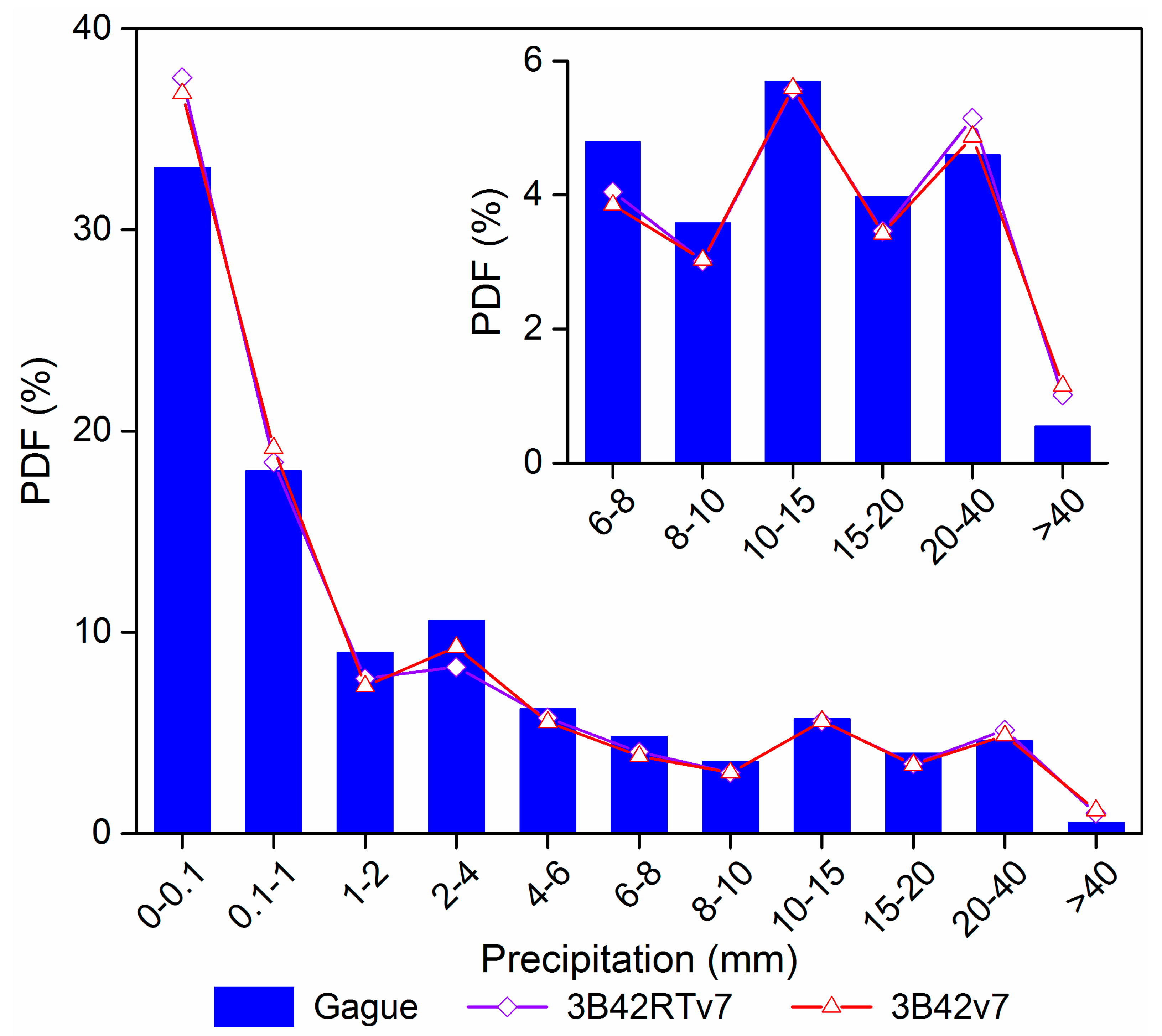
4.1. Evaluating the Consistency of Two SPE Products and Gauge-Based Reference

The agreement of three precipitation products was depicted by the spatial-temporal distribution and precipitation-intensity pattern. The spatial variations of daily average of SPE vs. Gauge precipitation showed the central region and area around Waizhou outlet with lower rainfall and regions in northwest, mid-east and most southwest with much higher rainfall across the Ganjiang River basin (Figure 3). Similar patterns were reported in previous studies on evaluating the adequacy of TRMM multi-satellite precipitation in the Ganjiang River basin [44,45]. Although the three datasets displayed broadly the same pattern of rainfall spatial distribution, there existed a slight difference in each of them. The estimates of daily average rainfall during 2000–2013 were 3.75–4.93 mm/d, 3.62–5.52 mm/d and 4.08–4.90 mm/d across the whole basin for gauge reference, 3B42RTv7 and 3B42v7, respectively. From the boxplot of Figure 3d, it was confirmed again that 3B42RTv7 showed a higher median and a larger inter-quartile range than the 3B42v7 and Gauge rainfall. While the lowest median and narrowest inter-quartile range were observed in Gauge rainfall indicating the smallest spatial variation in it.
The difference of three categorical statistics among 60 gauge stations was displayed in Figure 4, indicating good consistency between SPE used and Gauge reference data. The median values of POD are 0.59 and 0.62 for 3B42RTv7 and 3B42v7, respectively, compared to the Gauge data. 3B42v7 shows better performance of POD than 3B42RTv7 in most gauges (Figure 4a,b). Meanwhile, the higher POD of 3B42RTv7 and 3B42v7 are accompanied by lower FAR in those corresponding gauges (with median FAR values of 0.54 and 0.47 respectively). The ETS metric is more helpful to understand the overall detection ability of SPE. Most of ETS in Figure 4e,f (90%) are ranging from 0.22 to 0.39, from 0.23 to 0.41 for 3B42RTv7 and 3B42v7, respectively.
The space-averaged daily precipitation series keeps good consistency between the SPE and ground-based precipitation. The values of pairwise correlation, r, between three datasets were relatively high (greater than 0.88). In general, the performance of 3B42RTv7 and 3B42v7 products suggested by the Probability Density Function (PDF) of daily precipitation in Figure 5 was acceptable, compared to the gauge-based precipitation. The primary differences between the PDFs of SPE and gauge-based reference arose from the lower ends of precipitation intensity bins, where 3B42RTv7 and 3B42v7 overestimated the case of precipitation in 0–0.1 mm/d and 0.1–1 mm/d while underestimated that in 1–2 mm/d and 2–4 mm/d. As for moderate and heavy precipitation (>6.0 mm/d), the SPE, i.e., 3B42RTv7 and 3B42v7 datasets, showed closed PDFs relative to the gauge precipitation.

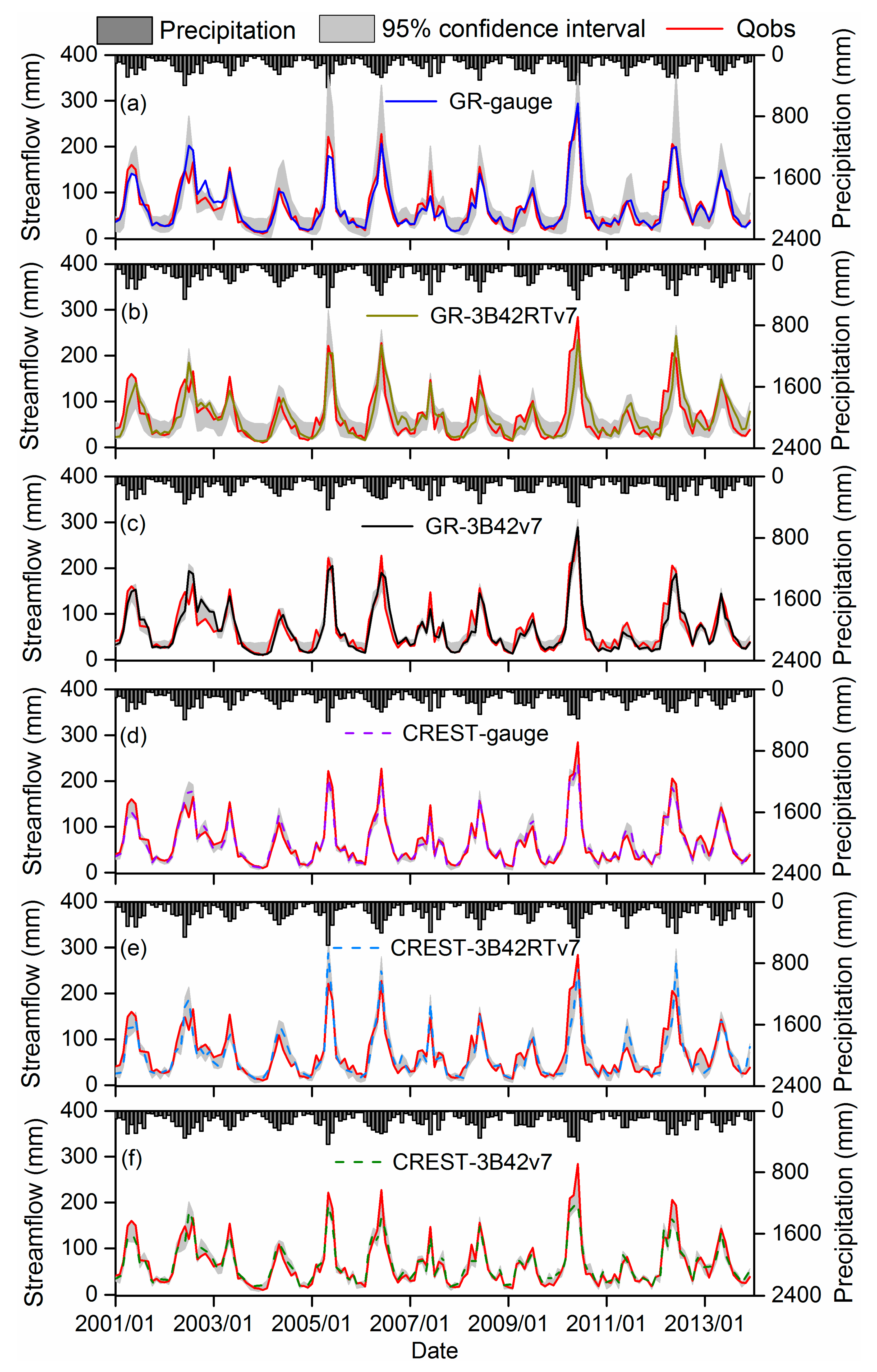
4.2. Hydrologic Evaluation of SPE

For rainfall-runoff models, bias in precipitation input can propagate into streamflow simulation and prediction, resulting in input uncertainty as well as uncertainties interactive with input through the hydrological processes [11]. In order to understand the impact of different precipitation datasets on hydrological effect, streamflow simulation by two hydrological models was carried out during 2000–2013.
For the gauge precipitation-forced GR model, GR6J obtained the highest NSE (0.83), followed by GR4J and GR5J (0.82 and 0.81). For the SPE-forced GR model, the calibrated GR6J also had the highest NSE among three model structures (with values of 0.67 and 0.77 for 3B42RTv7 and 3B42v7, respectively) (Table 3). As for the case of CREST, the NSE values derived from the model structure with varying expM parameter, i.e., CREST v1, were higher than those obtained from CREST v2 for all the three precipitation inputs. This result is reasonable as models with relatively more parameters generally have better fitness ability in the calibration. Furthermore, the simulated streamflow using both GR and CREST has relatively lower NSE and r values when driven by the SPE inputs, compared to the gauge-based input. However, for both models, 3B42v7 forced models (with NSE and r ranging from 0.72 to 0.77 and 0.85 to 0.88 respectively) performed significantly better than those forced by 3B42RTv7 (with NSE and r ranging from 0.49 to 0.68 and 0.75 to 0.82) (Table 3). As for the relative Bias, GR4J has least relative Bias among three GR structures for all three precipitation inputs, while the values of Bias of CREST v1 and v2 are comparable. All the Bias values are negative except for that of GR4J driven by gauge data.
For each of the two hydrological models and each of the three input scenarios, the 95CIs of ensemble outputs of simulated streamflow over all model structures, hypothetical precipitation levels and stochastic parameter sets were presented, providing a direct way to depict the interval information for outputs and the reliability of the modeling (Table 4 and Figure 6). Much narrower 95CIs were observed for the outputs derived from CREST driving by all the three precipitation inputs (Figure 6d–f), compared to the GR model (Figure 6a–c). It is clear that the band in 95CI around extreme values of the simulated streamflow over the study period was significantly wider than in other area. As for the quantitative indexes of the 95CI, 3B42v7-forced GR obtained best values of CR (63.46%), B (24.76 mm) and D (12.05 mm) among three inputs of GR model, while the 3B42RTv7-forced GR had the worst values of CR (58.97%), B (38.47 mm) and D (20.28 mm), and gauge rainfall-forced GR was with median performance. The CR, B and D indexes of CREST driven by the 3B42RTv7 also performed worst among three inputs, while CREST with Gauge precipitation input obtained best indexes, followed by the post-real-time satellite product 3B42v7. On the other hand, the distributed CREST model forced by three inputs generally obtained better CR, B and D indexes, relative to the lumped GR model. In summary, among six schemes combing two models with three precipitation inputs, CREST with Gauge precipitation performed best towards CR (81.41%), B (16.91 mm) and D (6.94 mm), followed by the CREST with 3B42v7.

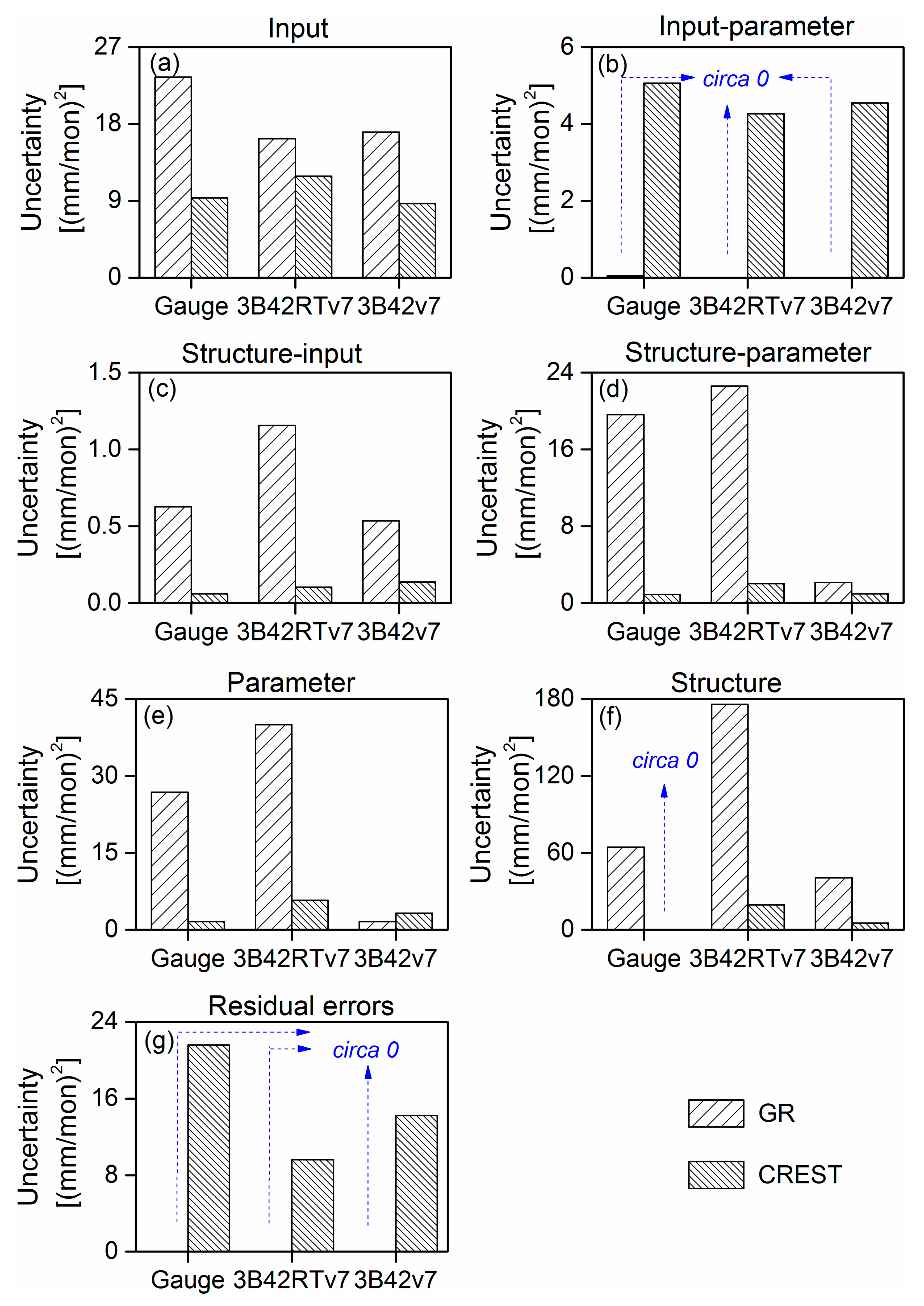
4.3. Variance-Based Uncertainty Component Analysis

4.3.1. Inter-comparison of Uncertainties in Precipitation Input with Other Sources

The fractional variance of seven uncertainty components partitioned based on variance decomposition method was presented for six combination schemes (over two models and three input scenarios of precipitation) (Figure 7). Generally, it can be observed that structure uncertainty dominated the total uncertainty in GR for all the three inputs (Figure 7a,c,e), while input uncertainty was the leading source of the total uncertainty in CREST (Figure 7b,d,f).The averaged fractional variance showed that the structure uncertainty contributed 38.59%, 53.22% and 60.81% to the total uncertainty in GR forced by Gauge precipitation, 3B42RTv7 and 3B42v7 respectively, whereas the contribution of structure uncertainty to the total uncertainty in CREST forced by these three inputs was below 27.04% (Figure 8). In contrast to the significant contribution of structure uncertainty in the GR model, the input uncertainty contributed 35.62%, 23.35% and 30.34% to the total uncertainty in CREST forced by Gauge precipitation, 3B42RTv7 and 3B42v7 respectively. The contributions of input uncertainty in CREST for three inputs were significantly greater, relative to GR with values smaller than 26.04%. In addition, the contribution of uncertainty stemming from parameter was relatively stable with values ranging from 19.41% to 27.10% among six combinations, except for the GR model driven by 3B42v7 (4.04%) (Figure 8). The uncertainty components from residual error are negligible in GR, in contrast to the significant impact on CREST.
The overall interaction effects had a significant contribution to the total uncertainty in all the six combination schemes with varying situations for each of the three interactions (Figure 8). For example, the interaction between structure and parameter, i.e., structure-parameter uncertainty, was more considerable in GR with all three inputs (ranging from 7.62% to 20.79%) than that in CREST (ranging from 3.52% to 7.43%). However, similar to the case of residual error, the input-parameter uncertainty is also approximate to zero in the GR model results, against an apparent influence to the CREST model with values ranging from 9.19% to 19.48%. As it is expected, the interaction between structure and input uncertainty in both the GR and CREST model was ignorable, whose contribution to total uncertainty was below 1.49%.
The inter-comparison of seven uncertainty components separated above in magnitude was conducted for two hydrological models combined with three inputs (Figure 9). Except for the input-parameter and residual error uncertainty, the other five components were overall significantly larger in GR model than those in CREST model for three input scenarios of precipitation. On the other hand, most uncertainty components derived from 3B42v7-driven models were smallest among three precipitation inputs for both the GR and CREST models.
In summary, the structure uncertainty in the result of GR had a dominantly larger percentage and magnitude compared to CREST, indicating the advantage of the distributed model CREST in model structure. Theoretically, this result is understandable since the distributed model can depict the real natural system in mathematical mechanisms and physical processes with more complexity. In addition, both the GR and CREST models forced by 3B42v7 performed better than those forced by gauge-based dataset towards seven uncertainty components in most cases, while the performance of both models forced by 3B42RTv7 was inferior to those by gauge-based dataset. This result suggested that the post-real-time TRMM product 3B42v7 was superior to the real-time TRMM product 3B42RTv7 towards uncertainty component evaluation.

4.3.2. Inter-comparison of Input Uncertainties among Six Schemes

Subsequently, average input uncertainties in streamflow simulation over six schemes (two models combined with three input scenarios) against three sources of precipitation on a monthly scale were provided in Figure 10. The three precipitation sources and two types of models exerted varying influences on input uncertainty in modeling. In general, input uncertainties in CREST with all three precipitation scenarios were much lower compared to those in GR. For both GR and CREST, the input uncertainty in result derived from 3B42v7 was much lower, compared to 3B42RTv7 and gauge-based precipitation. Input uncertainty in GR with gauge precipitation was highest in magnitude among six schemes, followed by those in GR with 3B42RTv7 and 3B42v7. It is obvious that monthly-averaged input uncertainties for all the six schemes increased from January to June, and decreased from June to December. Like the corresponding precipitation series, the input uncertainty series reached a peak in June.
Further, the correlations between input uncertainties separated from ensemble variance of streamflow simulation above and (a) corresponding precipitation datasets and (b) observed streamflow series were explored individually. As illustrated in Figure 11, the polynomial correlation was more realistic to depict the relationship of input uncertainty and precipitation or observed streamflow than the linear correlation. Overall, the fitness between input uncertainty and observed streamflow has better performance in terms of R2 (coefficient of determination), compared to input uncertainty and precipitation. In both cases of (a) and (b), R2 values of the fitted relationship were relatively high with values ranging from 0.71 to 0.87 for the precipitation (a) and from 0.71 to 0.89 for the observed streamflow (b). This demonstrated the applicability of the nonlinear relationship between input uncertainty and precipitation or streamflow, in which the magnitude of input uncertainty increased much faster than the precipitation or streamflow itself.

4.4. Discussion

Among six combination schemes discussed above, the scheme with good optimization results in model calibration may not have the same good performance in 95CI in the ensemble outputs. As an example, the NSE, r and Bias derived from the GR model forced by gauge precipitation were very satisfying, contrasting with low CR value as well as the high B and D values which indicated inferior 95CI. This phenomenon was also captured in previous studies. For example, in the result of Tian et al. [46] on applying the Xinanjiang model to the Jinhua River and Qu River, the average width of 90% confidence interval induced by varying parameters increased when the NSE became better. In addition, a similar result was found in Zeng et al. [47]. This suggested that although point estimate (e.g., NSE and r) can provide a way to quantify modeling precision, it cannot represent the modeling reliability in the sense of uncertain cases. Therefore, in addition to point estimate, the interval estimate is indispensable to quantify the reliability. In this sense, a trade-off between these two aspects should be taken into consideration simultaneously when choosing an optimal alternative input from different sources of precipitation products.
It is significantly beneficial to analyze the suitability of SPE precipitation data indirectly through hydrological modeling effect because the rainfall-runoff process integrates discrepancy in spatiality of precipitation into the bias of simulated streamflow at the transection of a river. In this integration process, the hydrological models can compensate the input data uncertainty arising from systematic error and/or random error. Knoche et al. [12] reported that more complex hydrological models were capable of better compensation for the error in input data. In the context of the present study, the CREST model driven by TRMM post-real-time product 3B42v7 generated minimal input uncertainty among all the six schemes. This is because the advantage of SPE lies on the spatially distributed precipitation at high resolution. Unlike lumped models, the distributed models calculate rainfall-runoff process based on a grid network, which makes better use of the spatial information of SPE. Accordingly, in this study, the distributed CREST hydrological model can give potential suitability and adequacy of high-quality satellite precipitation products especially for the post-real-time product 3B42v7, relative to the lumped GR model. Moreover, Knoche et al. [12] verified strong interdependence between input data and model structure on modeling performance. This study similarly confirmed the interdependence of precipitation input and model structure, whereas it is further proved that this interdependence is indirect. This is because the uncertainty component of the structure-input interaction was extremely low (around zero) in all the six schemes, against the significant structure-parameter and input-parameter interaction effects. Therefore, the model structure exerted influence on parameter and subsequently the parameter imposed restriction on precipitation, leading to the above interdependence as well as the compensation, and vice versa.
Compared to near-real-time 3B42RTv7 precipitation, the reliability and superiority of post-real-time research product 3B42v7 over Ganjiang River basin were proved by both simulation ability and input uncertainty induced. Both SPE products reproduced the daily rainfall regime and streamflow regime with similar performance of gauge-based precipitation. This result is consistent with many other studies on TRMM data. For example, as indicated by Liu [29], better performance of research grade 3B42v7 product in rain distribution was found over land at a global scale than that of the 3B42RTv7 product. Gao et al. [10] revealed that 3B42v7 outperformed 3B42RTv7 in streamflow prediction precision when forcing the CREST model used to two tributaries of upper Yangtze River. This is likely due to (1) merging multiple information sources and post-processing adjustment i.e., the monthly ground-based observation adjustment included in the 3B42v7 estimates, which results in 3B42v7 performing in a more robust and accuracy way than 3B42RTv7, and (2) the calendar month used for IR calibration period in 3B42v7, rather than a 30-day trailing accumulation in 3B42RTv7. Nevertheless, despite that the post-real-time product 3B42v7 is the valuable datum suitable for research, the near-time product 3B42RTv7, which is slightly inferior in hydrological effect, is still useful in practice. To improve the skill of the real-time satellite precipitation product in hydrological forecast, the biased satellite data can be statistically calibrated via a latent variable, i.e., rainfall multiplier, to partly correct the bias without ground observations [5,24]. Taking the distributed model CREST v1 as example, when the rainfall multiplier correcting near-time 3B42RTv7 data was considered in parameter calibration, the NSE of simulated streamflow increases by 3% reaching 0.72, relative to that without rainfall multiplier used.
The framework used in the present study incorporated finite combinations of fixed model structures, stochastically sampled hypothetical input levels and parameter sets in a factorial way, and thus it is not completely stochastic. This leads to the results somewhat relying on the configuration of the models. We acknowledge that the absolute magnitude of uncertainty components detected is design-dependent, which is a potential barrier to a full utility of variance decomposition analysis. Nevertheless, this study facilities both the comparison of relative contribution of input uncertainty with other uncertainty sources and the impact of various precipitation datasets used in different hydrological models on the input uncertainty, by means of specified highly representative scenarios. In general, the framework coupling variance decomposition method with ensemble outputs of the hydrological model is highly representative and can be used to analyze relative contributions of uncertainties in hydrological modeling with other models or in other study areas. Furthermore, both processes of resampling initial coarse TRMM data and interpolating ground-based reference data to gridded rainfall at fine scale are not exactly accurate, in which bias may arise. Further effort should be concentrated on this part to quantify its impact on the whole assessing framework.

5. Conclusions

This study systematically analyzed the associated uncertainties originating from two popular multi-sensor and multi-satellite precipitation estimates (i.e., TRMM Version-7 real-time product 3B42RTv7 and post-real-time research product 3B42v7) and gauge-based precipitation in hydrological utility using two hydrological models (the GR and CREST models). To quantify the relative contribution of input uncertainty and its interactions with parameter uncertainty and model structure uncertainty in streamflow modeling driven by the three precipitation datasets one by one as input, the variance decomposition method was applied to disaggregate the total uncertainty to seven components of potential sources. The total and fractional variances of seven uncertainty components partitioned were presented for six combination schemes (two hydrological models combined with three input scenarios of precipitation above).
The primary conclusions are summarized as follows: (1) For both the GR and CREST models, the 3B42v7-driven hydrological modeling towards the optimal simulation (NSE/r) and 95% confidence interval performed better compared to 3B42RTv7, whereas it was slightly inferior to those derived from gauge-based precipitation. (2) It was deduced that the total uncertainty in GR was lowest, moderate and highest when forced by gauge precipitation, 3B42v7 and 3B42RTv7, respectively. While the total uncertainty in CREST driven by 3B42v7 was lower relative to both 3B42RTv7 and interpolated precipitation from gauges. This result highlighted the superiority of post-real-time 3B42v7 to real-time 3B42RTv7 in hydrological modeling. (3) Among seven uncertainty components, input uncertainty dominated the total uncertainty in CREST for all the three precipitation inputs (contributing to 23.35% to 35.62%). Structure uncertainty was the leading source of the total uncertainty in GR for the three inputs (contributing to 38.59% to 60.81%). It emphasized the potential of the distributed model of compensating for the uncertain input data. (4) All the input uncertainties in CREST driven by 3B42v7, 3B42RTv7 and gauge-based precipitation were lower than those in GR. Among six combination schemes, the input uncertainty was lowest in the 3B42v7-driven CREST model while highest in the gauge-based precipitation-driven GR model. This result demonstrated that the distributed CREST model is capable of making better use of the spatial distribution advantage of SPE.
Consequently, this study reveals new insights into satellite precipitation-induced input uncertainty and its interactions with other uncertainties in hydrological utility. The results and conclusions indeed illustrate the promising prospect of applying satellite precipitation products towards hydrological modeling in the sense of both modeling precision and reliability.

Author Contributions

Q.M. and L.X. designed the experiments; Q.M. performed the experiments, analyzed the data and wrote the original draft; C.-Y.X. provided helpful suggestions; D.L. and S.G. polished the document.

Funding

This study has received funding from The National Key Research and Development Program of China (Grants No. 2017YFC0405901) and National Natural Science Foundation of China (Grants Nos. 51525902 and 51479139).

Acknowledgments

Partial hydrological and meteorological data were provided by hydrological bureau of Jiangxi province, who we shall acknowledge for sharing data.

Conflicts of Interest

The authors declare no conflict of interest.

References

  1. Katiraie-Boroujerdy, P.; Asanjan, A.A.; Hsu, K.; Sorooshian, S. Intercomparison of PERSIANN-CDR and TRMM-3B42V7 precipitation estimates at monthly and daily time scales. Atmos. Res. 2017, 193, 36–49. [Google Scholar] [CrossRef]
  2. Sunilkumar, K.; Rao, T.N.; Satheeshkumar, S. Assessment of small-scale variability of rainfall and multi-satellite precipitation estimates using measurements from a dense rain gauge network in Southeast India. Hydrol. Earth Syst. Sci. 2016, 20, 1719–1735. [Google Scholar] [CrossRef] [Green Version]
  3. Renard, B.; Kavetski, D.; Kuczera, G.; Thyer, M.; Franks, S.W. Understanding predictive uncertainty in hydrologic modeling: The challenge of identifying input and structural errors. Water Resour. Res. 2010, 46, W5521. [Google Scholar] [CrossRef]
  4. McMillan, H.; Jackson, B.; Clark, M.; Kavetski, D.; Woods, R. Rainfall uncertainty in hydrological modelling: An evaluation of multiplicative error models. J. Hydrol. 2011, 400, 83–94. [Google Scholar] [CrossRef]
  5. Yen, H.; Su, Y.; Wolfe, J.E.; Chen, S.; Hsu, Y.; Tseng, W.; Brady, D.M.; Jeong, J.; Arnold, J.G. Assessment of input uncertainty by seasonally categorized latent variables using SWAT. J. Hydrol. 2015, 531, 685–695. [Google Scholar] [CrossRef] [Green Version]
  6. Mockler, E.M.; Chun, K.P.; Sapriza-Azuri, G.; Bruen, M.; Wheater, H.S. Assessing the relative importance of parameter and forcing uncertainty and their interactions in conceptual hydrological model simulations. Adv. Water Resour. 2016, 97, 299–313. [Google Scholar] [CrossRef]
  7. Yong, B.; Hong, Y.; Ren, L.L.; Gourley, J.J.; Huffman, G.J.; Chen, X.; Wang, W.; Khan, S.I. Assessment of evolving TRMM-based multisatellite real-time precipitation estimation methods and their impacts on hydrologic prediction in a high latitude basin. J. Geophys. Res. Atmos. 2012, 117, D9108. [Google Scholar] [CrossRef]
  8. Gebregiorgis, A.S.; Tian, Y.; Peters Lidard, C.D.; Hossain, F. Tracing hydrologic model simulation error as a function of satellite rainfall estimation bias components and land use and land cover conditions. Water Resour. Res. 2012, 48, W11509. [Google Scholar] [CrossRef]
  9. Li, D.; Christakos, G.; Ding, X.; Wu, J. Adequacy of TRMM satellite rainfall data in driving the SWAT modeling of Tiaoxi catchment (Taihu lake basin, China). J. Hydrol. 2018, 556, 1139–1152. [Google Scholar] [CrossRef]
  10. Gao, Z.; Long, D.; Tang, G.; Zeng, C.; Huang, J.; Hong, Y. Assessing the potential of satellite-based precipitation estimates for flood frequency analysis in ungauged or poorly gauged tributaries of China’s Yangtze River basin. J. Hydrol. 2017, 550, 478–496. [Google Scholar] [CrossRef]
  11. Tong, K.; Su, F.; Yang, D.; Hao, Z. Evaluation of satellite precipitation retrievals and their potential utilities in hydrologic modeling over the Tibetan Plateau. J. Hydrol. 2014, 519, 423–437. [Google Scholar] [CrossRef]
  12. Knoche, M.; Fischer, C.; Pohl, E.; Krause, P.; Merz, R. Combined uncertainty of hydrological model complexity and satellite-based forcing data evaluated in two data-scarce semi-arid catchments in Ethiopia. J. Hydrol. 2014, 519, 2049–2066. [Google Scholar] [CrossRef]
  13. Li, Z.; Yang, D.; Gao, B.; Jiao, Y.; Hong, Y.; Xu, T. Multiscale Hydrologic Applications of the Latest Satellite Precipitation Products in the Yangtze River Basin using a Distributed Hydrologic Model. J. Hydrometeorol. 2015, 16, 407–426. [Google Scholar] [CrossRef]
  14. Yang, Z.; Hsu, K.; Sorooshian, S.; Xu, X.; Braithwaite, D.; Zhang, Y.; Verbist, K.M. Merging High-resolution Satellite-based Precipitation Fields and Point-scale Rain-gauge Measurements—A Case Study in Chile. J. Geophys. Res. Atmos. 2017, 122, 5267–5284. [Google Scholar] [CrossRef]
  15. Jing, W.; Yang, Y.; Yue, X.; Zhao, X. A spatial downscaling algorithm for satellite-based precipitation over the Tibetan plateau based on NDVI, DEM, and land surface temperature. Remote Sens. 2016, 8, 655. [Google Scholar] [CrossRef]
  16. Maggioni, V.; Sapiano, M.R.; Adler, R.F. Estimating uncertainties in high-resolution satellite precipitation products: Systematic or random error? J. Hydrometeorol. 2016, 17, 1119–1129. [Google Scholar] [CrossRef]
  17. Yong, B.; Chen, B.; Tian, Y.; Yu, Z.; Hong, Y. Error-component analysis of TRMM-based multi-satellite precipitation estimates over Mainland China. Remote Sens. 2016, 8, 440. [Google Scholar] [CrossRef]
  18. Maggioni, V.; Nikolopoulos, E.I.; Anagnostou, E.N.; Borga, M. Modeling satellite precipitation errors over mountainous terrain: The influence of gauge density, seasonality, and temporal resolution. IEEE Trans. Geosci. Remote Sens. 2017, 55, 4130–4140. [Google Scholar] [CrossRef]
  19. Shah, H.L.; Mishra, V. Uncertainty and bias in satellite-based precipitation estimates over indian subcontinental basins: Implications for real-time streamflow simulation and flood prediction. J. Hydrometeorol. 2016, 17, 615–636. [Google Scholar] [CrossRef]
  20. Mendoza, P.A.; Clark, M.P.; Mizukami, N.; Gutmann, E.D.; Arnold, J.R.; Brekke, L.D.; Rajagopalan, B. How do hydrologic modeling decisions affect the portrayal of climate change impacts? Hydrol. Process. 2016, 30, 1071–1095. [Google Scholar] [CrossRef]
  21. Sapriza Azuri, G.; Jódar, J.; Navarro, V.; Slooten, L.J.; Carrera, J.; Gupta, H.V. Impacts of rainfall spatial variability on hydrogeological response. Water Resour. Res. 2015, 51, 1300–1314. [Google Scholar] [CrossRef] [Green Version]
  22. Li, M.; Yang, D.; Chen, J.; Hubbard, S.S. Calibration of a distributed flood forecasting model with input uncertainty using a Bayesian framework. Water Resour. Res. 2012, 48, W8510. [Google Scholar] [CrossRef]
  23. Kavetski, D.; Kuczera, G.; Franks, S.W. Bayesian analysis of input uncertainty in hydrological modeling: 1. Theory. Water Resour. Res. 2006, 42, W3407. [Google Scholar] [CrossRef]
  24. Ajami, N.K.; Duan, Q.; Sorooshian, S. An integrated hydrologic Bayesian multimodel combination framework: Confronting input, parameter, and model structural uncertainty in hydrologic prediction. Water Resour. Res. 2007, 43, W1403. [Google Scholar] [CrossRef]
  25. Addor, N.; Rössler, O.; Köplin, N.; Huss, M.; Weingartner, R.; Seibert, J. Robust changes and sources of uncertainty in the projected hydrological regimes of Swiss catchments. Water Resour. Res. 2014, 50, 7541–7562. [Google Scholar] [CrossRef] [Green Version]
  26. Ren, Z.H.; Zhao, P.; Zhang, Q.; Zhang, Z.F.; Cao, L.J.; Yang, Y.R.; Zou, F.L.; Zhao, Y.F.; Zhao, H.M.; Chen, Z. Quality control procedures for hourly precipitation data from automatic weather stations in China. Meteorol. Mon. 2010, 36, 123–132. [Google Scholar]
  27. Gebremichael, M.; Hossain, F. Satellite Rainfall Applications for Surface Hydrology; Springer: Berlin, Germany, 2010; pp. 3–22. [Google Scholar]
  28. Huffman, G.J.; Bolvin, D.T. TRMM and Other Data Precipitation Data Set Documentation; NASA: Greenbelt, MD, USA, 2013; Volume 28, pp. 1–46.
  29. Liu, Z. Comparison of precipitation estimates between Version 7 3-hourly TRMM Multi-Satellite Precipitation Analysis (TMPA) near-real-time and research products. Atmos. Res. 2015, 153, 119–133. [Google Scholar] [CrossRef]
  30. Bowman, K.P.; Hong, Y.; Stocker, E.F.; Wol, D.B. The TRMM multi-satellite precipitation analysis: Quasi-global, multi-year, combined-sensor precipitation estimates at finescale. J. Hydrometeorol. 2007, 8, 3855. [Google Scholar]
  31. Coron, L.; Perrin, C.; Delaigue, O.; Andréassian, V.; Thirel, G. airGR: A suite of lumped hydrological models in an R-package. Environ. Modell. Softw. 2017, 94, 166–171. [Google Scholar] [CrossRef]
  32. Shin, M.; Kim, C. Assessment of the suitability of rainfall-runoff models by coupling performance statistics and sensitivity analysis. Hydrol. Res. 2017, 48, 1192–1213. [Google Scholar] [CrossRef]
  33. Pushpalatha, R.; Perrin, C.; Le Moine, N.; Mathevet, T.; Andréassian, V. A downward structural sensitivity analysis of hydrological models to improve low-flow simulation. J. Hydrol. 2011, 411, 66–76. [Google Scholar] [CrossRef]
  34. Khan, S.I.; Adhikari, P.; Hong, Y.; Vergara, H.; F Adler, R.; Policelli, F.; Irwin, D.; Korme, T.; Okello, L. Hydroclimatology of Lake Victoria region using hydrologic model and satellite remote sensing data. Hydrol. Earth Syst. Sci. 2011, 15, 107–117. [Google Scholar] [CrossRef] [Green Version]
  35. Khan, S.I.; Hong, Y.; Wang, J.; Yilmaz, K.K.; Gourley, J.J.; Adler, R.F.; Brakenridge, G.R.; Policelli, F.; Habib, S.; Irwin, D. Satellite remote sensing and hydrologic modeling for flood inundation mapping in Lake Victoria basin: Implications for hydrologic prediction in ungauged basins. IEEE Trans. Geosci. Remote Sens. 2011, 49, 85–95. [Google Scholar] [CrossRef]
  36. Wang, J.; Hong, Y.; Li, L.; Gourley, J.J.; Khan, S.I.; Yilmaz, K.K.; Adler, R.F.; Policelli, F.S.; Habib, S.; Irwn, D. The coupled routing and excess storage (CREST) distributed hydrological model. Hydrol. Sci. J. 2011, 56, 84–98. [Google Scholar] [CrossRef] [Green Version]
  37. Perrin, C.; Michel, C.; Andréassian, V. Improvement of a parsimonious model for streamflow simulation. J. Hydrol. 2003, 279, 275–289. [Google Scholar] [CrossRef]
  38. Duan, Q.; Sorooshian, S.; Gupta, V. Effective and efficient global optimization for conceptual rainfall-runoff models. Water Resour. Res. 1992, 28, 1015–1031. [Google Scholar] [CrossRef]
  39. Yip, S.; Ferro, C.A.; Stephenson, D.B.; Hawkins, E. A simple, coherent framework for partitioning uncertainty in climate predictions. J. Clim. 2011, 24, 4634–4643. [Google Scholar] [CrossRef]
  40. Lovenduski, N.S.; McKinley, G.A.; Fay, A.R.; Lindsay, K.; Long, M.C. Partitioning uncertainty in ocean carbon uptake projections: Internal variability, emission scenario, and model structure. Glob. Biogeochem. Cycles 2016, 30, 1276–1287. [Google Scholar] [CrossRef]
  41. Guo, H.; Chen, S.; Bao, A.; Behrangi, A.; Hong, Y.; Ndayisaba, F.; Hu, J.; Stepanian, P.M. Early assessment of integrated multi-satellite retrievals for global precipitation measurement over China. Atmos. Res. 2016, 176, 121–133. [Google Scholar] [CrossRef]
  42. Wȩglarczyk, S. The interdependence and applicability of some statistical quality measures for hydrological models. J. Hydrol. 1998, 206, 98–103. [Google Scholar] [CrossRef]
  43. Xiong, L.; Wan, M.; Wei, X.; O’Connor, K.M. Indices for assessing the prediction bounds of hydrological models and application by generalised likelihood uncertainty estimation/Indices pour évaluer les bornes de prévision de modèles hydrologiques et mise en œuvre pour une estimation d’incertitude par vraisemblance généralisée. Hydrol. Sci. J. 2009, 54, 852–871. [Google Scholar]
  44. Tang, G.; Li, Z.; Xue, X.; Hu, Q.; Yong, B.; Hong, Y. A study of substitutability of TRMM remote sensing precipitation for gauge-based observation in Ganjiang River basin. Adv. Water Sci. 2015, 26, 340–346. [Google Scholar]
  45. Jiang, S.; Zhang, Z.; Huang, Y.; Chen, X.; Chen, S. Evaluating the TRMM Multisatellite Precipitation Analysis for Extreme Precipitation and Streamflow in Ganjiang River Basin, China. Adv. Meteorol. 2017, 2017, 2902493. [Google Scholar] [CrossRef]
  46. Tian, Y.; Booij, M.J.; Xu, Y. Uncertainty in high and low flows due to model structure and parameter errors. Stoch. Environ. Res. Risk Access. 2014, 28, 319–332. [Google Scholar] [CrossRef]
  47. Zeng, Q.; Chen, H.; Xu, C.; Jie, M.; Hou, Y. Feasibility and uncertainty of using conceptual rainfall-runoff models in design flood estimation. Hydrol. Res. 2016, 47, 701–717. [Google Scholar] [CrossRef]
Figure 1. Geographical location, topography, rainfall gauges, pan evaporation stations and discharge station of the study area.
Remotesensing 10 01876 g001
Figure 2. Overall framework of assessing the satellite precipitation estimate and quantifying its input uncertainty in driving hydrological models using the variance decomposition method.
Remotesensing 10 01876 g002
Figure 3. Spatial distributions of daily-averaged (a) interpolated gauge reference data, (b) 3B42RTv7 and (c) 3B42v7 (units in mm) with 0.25° × 0.25° spatial resolution during 14 years of study period from January 2000 to December 2013, as well as (d) boxplot summarizing the basin-averaged precipitation during the study period.
Remotesensing 10 01876 g003
Figure 4. Spatial distributions of (a,b) Probability of Detection (POD), (c,d) False Alarm Ratio (FAR), and (e,f) Equitable Threat Score (ETS) for 3B42RTv7 (the first column) and 3B42v7 (the second column) at a daily scale over the Ganjiang River basin for the 14-year study period (January 2000 to December 2013).
Remotesensing 10 01876 g004
Figure 5. Probability density function (PDF) of daily precipitation classified by different intensities, as derived from 3B42RTv7, 3B42v7 and gauge datasets over 2000–2013. The small panel in the upper right corner descripted the PDF of daily precipitation more than 6.0 mm.
Remotesensing 10 01876 g005
Figure 6. The 95% confidence intervals of the ensemble output for discharge of two models in three precipitation input scenarios. Qobs represents the observed discharge.
Remotesensing 10 01876 g006
Figure 7. Fractional variances (FV) of seven uncertainty components for each of the combination schemes of two models and three precipitation input scenarios. The first three subplots represent the combinations of GR with gauge-based precipitation, 3B42RTv7 and 3B42v7 input; the fourth to sixth subplots represent the combinations of CREST with these three inputs.
Remotesensing 10 01876 g007
Figure 8. Stacked histogram of respective relative contribution of seven uncertainty components to the total uncertainty.
Remotesensing 10 01876 g008
Figure 9. Comparison of the individual uncertainties from seven sources in the GR and CREST models.
Remotesensing 10 01876 g009
Figure 10. Time series of monthly-averaged input uncertainty and the histogram of three categories of precipitation datasets in monthly scale during the study period.
Remotesensing 10 01876 g010
Figure 11. Scatter plots of input uncertainty against (a) gauge-based precipitation, (b) 3B42RTv7, (c) 3B42v7 and (d) the observed streamflow at monthly scale with the result of polynomial fitness.
Remotesensing 10 01876 g011
Table 1. Summary of parameter information for the Génie Rural (GR) and Coupled Routing and Excess STorage (CREST) models.
SymbolDescriptionNumerical RangeUnit
GRX1Production store capacity100–1400mm
X2Intercatchment exchange coefficient−4–4mm/d
X3Routing store capacity0–500mm
X4Unit hydrograph time constant0–10d
X5Intercatchment exchange threshold−4–4
X6Coefficient for emptying exponential store0–20mm
CRESTKsatThe soil saturate hydraulic conductivity10–3000mm/d
WMThe mean water capacity80–200mm
BThe exponent of the variable infiltration curve0.05–1.5
IMImpervious area ratio0–0.2
KEThe factor to convert the potential evapotranspiration to local actual0.1–1.5
coeMOverland runoff velocity coefficient1.0–150
expMOverland flow speed exponent0.1–2.0
coeRMultiplier used to convert overland flow speed to channel flow speed1.0–3.0
coeSMultiplier used to convert overland flow speed to interflow speed0.001–1.0
KSOverland reservoir discharge parameter0–1.0
KIInterflow reservoir discharge parameter0–1.0
Table 2. Decomposition of total uncertainty into seven components using the variance decomposition method.
Sources of UncertaintyDifference/VarianceExpression
Input from precipitation (I)Difference Δ I i = Y i .. Y
Variance U I 2 = 1 N I i ( Δ I i Δ I i ¯ ) 2
Parameter set (P)Difference Δ P j = Y . j . Y
Variance U P 2 = 1 N P j ( Δ P j Δ P j ¯ ) 2
Model structure (S)Difference Δ S k = Y .. k Y
Variance U S 2 = 1 N S k ( Δ S k Δ S k ¯ ) 2
Interaction between input and parameter (IP)Difference Δ I P i j = Y i j . Y i .. Y . j . + Y
Variance U I P 2 = 1 N I N P i j ( Δ I P i j Δ I P i j ¯ ) 2
Interaction between input and structure (IS)Difference Δ I S i k = Y i . k Y i .. Y .. k + Y
Variance U I S 2 = 1 N I N S i k ( Δ I S i k Δ I S i k ¯ ) 2
Interaction between parameter and structure (PS)Difference Δ P S j k = Y . j k Y . j . Y .. k + Y
Variance U P S 2 = 1 N P N S j k ( Δ P S j k Δ P S j k ¯ ) 2
Residual error (v)Difference ε i j k = Y i j k Y i .. Y . j . Y . k . + 2 Y
Variance U v 2 = 1 N I N P N S i j k ( ε i j k ε i j k ¯ ) 2
Note: A bar denotes averaging and the dots indicate which component has been averaged.
Table 3. Optimal criteria in model calibration.
Gauge3B42RTv73B42v7
NSErBias (%)NSErBias (%)NSErBias (%)
GR4J0.820.910.660.610.78−0.130.750.87−2.16
GR5J0.810.91−6.580.660.82−6.040.760.88−7.03
GR6J0.830.91−6.530.670.82−6.840.770.88−7.30
CREST v10.860.93−2.490.680.83−3.830.740.86−1.57
CREST v20.860.93−2.490.490.75−3.830.720.85−1.98
Table 4. Statistical indexes for interval estimation.
GRCREST
CR (%)B (mm)D (mm)CR (%)B (mm)D (mm)
Gauge58.9738.4720.2881.4116.916.94
3B42RTv771.7952.4220.4947.4420.8715.84
3B42v763.4624.7612.0577.5620.638.53
Note: The optimal CR value is 100, the optimal B and D values are 0.

