Mapping Ecological Production and Benefits from Water Consumed in Agricultural and Natural Landscapes: A Case Study of the Pangani Basin

 ,
,
Abstract
:
1. Introduction
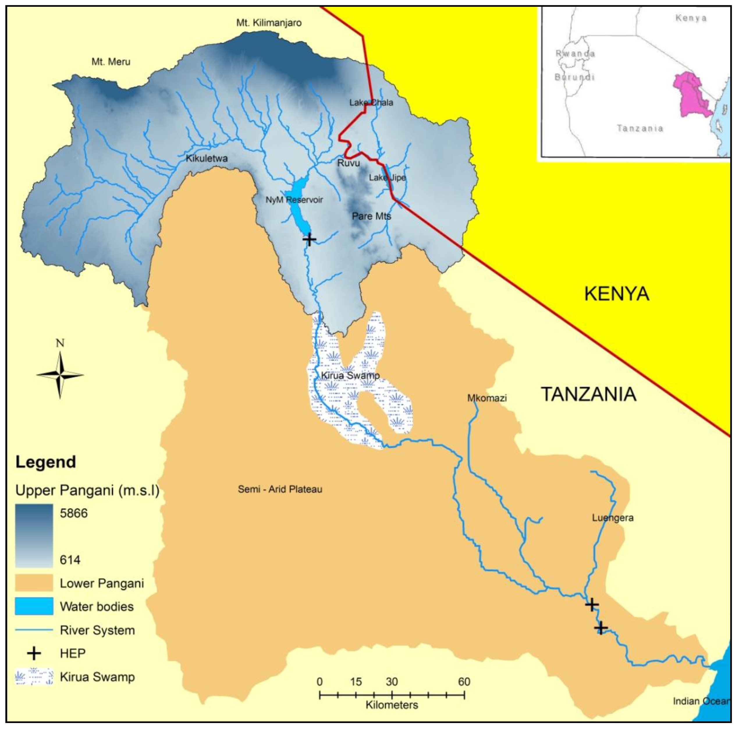
2. Study Area
3. Materials and Methods
3.1. Remotely-Sensed Data for Assessing Ecological Productivity
3.1.1. Actual Evaporation
3.1.2. Biomass Production
3.1.3. Crop Yield
3.1.4. Carbon Sequestration
3.1.5. Economic Water Productivity
3.2. Boundary Conditions for Water Productivity Assessment
3.3. Calibration and Validation
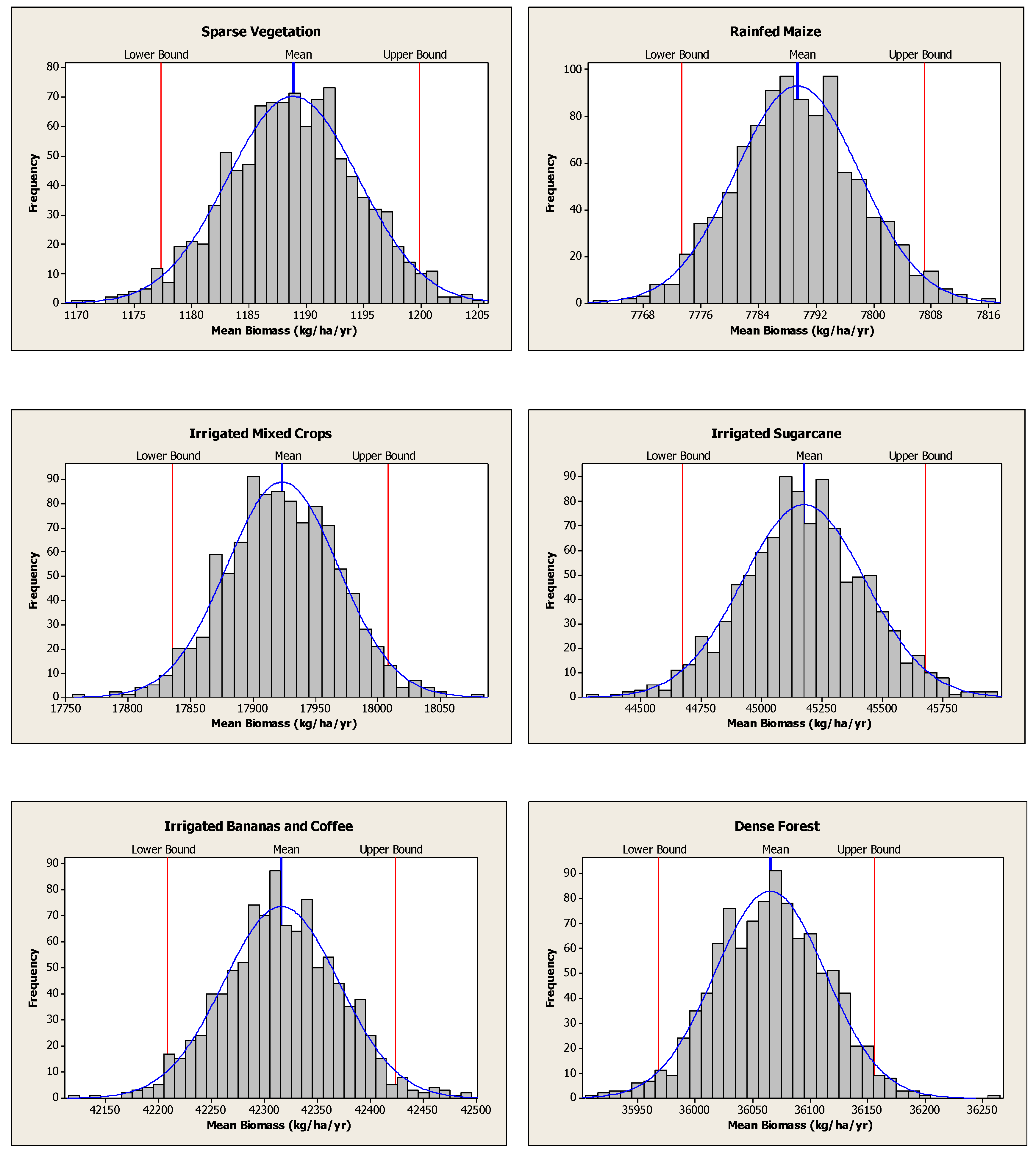
3.4. Uncertainty Analysis of Biomass Production
4. Results
4.1. Biomass Production
4.2. Variability in Biomass Production
4.3. Water Yield
4.4. Water Productivity
4.4.1. Biomass and Crop Water Productivity
4.4.2. Economic Water Productivity
4.4.3. Economic Water Productivity for Irrigation Water Use
5. Discussion
6. Conclusions
Supplementary Materials
Author Contributions
Funding
Acknowledgments
Conflicts of Interest
References
- De Fraiture, C.; Giordano, M.; Liao, Y. Biofuels and implications for agricultural water use: Blue impacts of green energy. Water Policy 2008, 10, 67–81. [Google Scholar] [CrossRef]
- Millennium Ecosystem Assessment. Ecosystems and Human Well-Being: Current States and Trends; Island Press: Washington, DC, USA, 2005. [Google Scholar]
- De Groot, R.; Brander, L.; van der Ploeg, S.; Costanza, R.; Bernard, F.; Braat, L.; Christie, M.; Crossman, N.; Ghermandi, A.; Hein, L.; et al. Global estimates of the value of ecosystems and their services in monetary units. Ecosyst. Serv. 2012, 1, 50–61. [Google Scholar] [CrossRef] [Green Version]
- Rockström, J.; Gordon, L.; Folke, C.; Falkenmark, M.; Engwall, M. Linkages among water vapor flows, food production, and terrestrial ecosystem services. Conserv. Ecol. 1999, 3, 5. [Google Scholar] [CrossRef]
- Wackernagel, M.; Onisto, L.; Bello, P.; Linares, A.C.; Falfán, I.S.L.; García, J.M.; Guerrero, A.I.S. National natural capital accounting with the ecological footprint concept (Analysis). Ecol. Econ. 1999, 29, 375–390. [Google Scholar] [CrossRef]
- Monfreda, C.; Wackernagel, M.; Deumling, D. Establishing national capital accounts based on detailed Ecological Footprint and biological capacity assessments. Land Use Policy 2004, 21, 231–246. [Google Scholar] [CrossRef]
- Karimi, P.; Bastiaanssen, W.G.M.; Sood, A.; Hoogeveen, J.; Peiser, L.; Bastidas-Obando, E.; Dost, R.J. Spatial evapotranspiration, rainfall and landuse data in water accounting results for policy decisions in the Awash Basin. Hydrol. Earth Syst. Sci. 2015, 19, 533–550. [Google Scholar] [CrossRef]
- Bastiaanssen, W.G.M.; Karimi, P.; Rebelo, L.; Duan, Z.; Senay, G.; Muthuwatte, L.; Smakhtin, V. Earth observation based assessment of the water production and water consumption of Nile Basin Agro-Ecosystems. Remote Sens. 2014, 6, 10306–10334. [Google Scholar] [CrossRef]
- Kijne, J.W.; Barker, R.; Molden, D.J. (Eds.) Economics of water productivity in managing water for agriculture. In Water Productivity in Agriculture—Limits and Opportunities for Improvements, Comprehensive Assessment of Water Management in Agriculture; CABI Publishing in Association with International Water Management Institute: Wallingford, UK, 2003; pp. 19–35. [Google Scholar]
- Rodríguez-Ferrero, N. Water productivity in irrigation systems. Water Int. 2003, 28, 341–349. [Google Scholar] [CrossRef]
- Ali, M.H.; Hoque, M.R.; Hassan, A.A.; Khair, A.A. Effects of deficit irrigation on wheat yield, water productivity and economic returns. Agric. Water Manag. 2007, 92, 151–161. [Google Scholar] [CrossRef]
- Hellegers, P.J.G.J.; Soppe, R.; Perry, C.J.; Bastiaanssen, W.G.M. Combining remote sensing and economic analysis to support decisions that affect water productivity. Irrig. Sci. 2009, 27, 243–251. [Google Scholar] [CrossRef]
- . Food and Agricultural Organization of the United Nations (FAO). Payments for Ecosystem Services and Food Security; Food and Agricultural Organization of the United Nations: Rome, Italy, 2011; 300p, ISBN 978-92-5-106796-3. [Google Scholar]
- Enfors, E.; Gordon, L. Dealing with drought: The challenge of using water system technologies to break dryland poverty traps. Glob. Environ. Chang. 2008, 18, 607–616. [Google Scholar] [CrossRef]
- IUCN. The Pangani River Basin: A Situation Analysis, 2nd ed.; IUCN Eastern Africa Region Office: Nairobi, Kenya, 2009. [Google Scholar]
- Costanza, R.; de Groot, R.S.; Sutton, P.; van der Ploeg, S.; Anderson, S.J.; Kubiezewski, I.; Farber, I.; Turner, R.K. Changes in the global value of ecosystem services. Glob. Environ. Chang. 2014, 26, 152–158. [Google Scholar] [CrossRef]
- Stubbs, M. Conservation Reserve Program (CRP): Status and Issues; Congressional Research Service: Washington, DC, USA, 2014. [Google Scholar]
- Saah, D.; Troy, A. Developing an Ecosystem Service Value Baseline; USAID Cooperative Agreement No. AID-486-A-12-00009; Vietnam Forests and Deltas Program: Hanoi, Vietnam, 2015. [Google Scholar]
- Keller, J.; Keller, A.; Davids, G. River basin development phases and implications of closure. J. Appl. Irrig. Sci. 1998, 33, 145–163. [Google Scholar]
- Igbadun, H.E.; Mahoo, H.F.; Tarimo, A.K.P.R.; Salim, B.A. Crop water productivity of an irrigated maize crop in Mkoji sub-catchment of the Great Ruaha River Basin, Tanzania. Agric. Water Manag. 2006, 85, 141–150. [Google Scholar] [CrossRef]
- Karimi, P.; Bastiaanssen, W.G.M.; Molden, D.J.; Cheema, M.J. Basin-wide water accounting based on remote sensing data: an application for the Indus Basin. Hydrol. Earth Syst. Sci. 2013, 17, 2473–2586. [Google Scholar] [CrossRef]
- Yokwe, S. Water productivity in smallholder irrigation schemes in South Africa. Agric. Water Manag. 2009, 96, 1223–1228. [Google Scholar] [CrossRef]
- Molden, D.; Oweis, T.Y.; Steduto, P.; Kijne, J.W.; Hanjra, M.A.; Bindraban, P.S. Pathways for increasing agricultural water productivity. In Water for Food, Water for Life: A Comprehensive Assessment of Water Management in Agriculture; Earthscan: London, UK; International Water Management Institute: Colombo, Sri Lanka, 2007. [Google Scholar]
- Van der Zaag, P. Viewpoint—Water variability, soil nutrient heterogeneity and market volatility—Why sub-Saharan Africa’s Green Revolution will be location-specific and knowledge-intensive. Water Altern. 2010, 3, 154–160. [Google Scholar]
- Bossio, D.; Jewitt, G.; van der Zaag, P. Editorial—Smallholder system innovation for integrated watershed management in Sub-Saharan Africa. Agric. Water Manag. 2011, 98, 1683–1686. [Google Scholar] [CrossRef]
- Fereres, E.; Orgaz, F.; Gonzalez-Dugo, V.; Testi, L.; Villalobos, F.J. Balancing crop yield and water productivity tradeoffs in herbaceous and woody crops. Funct. Plant Boil. 2014, 41, 1009–1018. [Google Scholar] [CrossRef]
- Molden, D.; Sakthivadivel, R. Water Accounting to Assess Use and Productivity of Water. Int. J. Water Resour. Dev. 1999, 15, 55–71. [Google Scholar] [CrossRef]
- Molden, D.; Oweis, T.Y.; Steduto, P.; Bindraban, P.; Hanjra, M.A.; Kijne, J. Improving agricultural water productivity: Between optimism and caution. Agric. Water Manag. 2010, 97, 528–535. [Google Scholar] [CrossRef]
- Kijne, J.; Barron, J.; Hoff, H.; Rockström, J.; Karlberg, L.; Gowing, J.; Wani, S.P.; Wichelns, D. Opportunities to Increase Water Productivity in Agriculture with Special Reference to Africa and South Asia; A Report Prepared by Stockholm Environment Institute, for the Swedish Ministry of Environment Presentation at CSD 16, N. Y. 14 May 2009; Stockholm Environment Institute: Stockholm, Sweden, 2009; 39p. [Google Scholar]
- Costanza, R.; d’Arge, R.; de Groot, R.; Farber, S.; Grasso, M.; Hannon, B.; Limburg, K.; Naeem, S.; O’Neill, R.V.; Paruelo, J.; et al. The value of the world’s ecosystem services and natural capital. Nature 1997, 387, 253–260. [Google Scholar] [CrossRef]
- Hermans, L.M.; van Halsema, E.G.; Mahoo, F.H. Building a mosaic of values to support local water resources management. Water Policy 2006, 8, 415–434. [Google Scholar] [CrossRef]
- Enfors, E.; Gordon, L. Analysing resilience in dryland agro-ecosystems: A case study of the Makanya catchment in Tanzania over the past 50 years. Land Degrad. Dev. 2007, 18, 680–696. [Google Scholar] [CrossRef]
- Batjes, N.H. Projected changes in soil organic carbon stocks upon adoption of recommended soil and water conservation practices in the Upper Tana River catchment, Kenya. Land Degrad. Dev. 2014, 35, 278–287. [Google Scholar] [CrossRef]
- Sedjo, R.A. Forest Carbon Sequestration: Some Issues for Forest Investments; Discussion Paper No. 01-34; Resources for the Future: Washington, DC, USA, 2001. [Google Scholar]
- Pizer, W.A. Combining price and quantity controls to mitigate global climate change. J. Public Econ. 2002, 85, 409–434. [Google Scholar] [CrossRef]
- Stern, N. The Economics of Climate Change: The Stern Review; Cambridge University Press: Cambridge, UK; New York, NY, USA, 2007. [Google Scholar]
- Zwart, S.J.; Bastiaanssen, W.G.M. SEBAL for detecting spatial variation of water productivity and scope for improvement in eight irrigated wheat systems. Agric. Water Manag. 2007, 89, 287–296. [Google Scholar] [CrossRef]
- Van Dam, J.C.; Singh, R.; Bessembinder, J.J.E.; Leffelaar, P.A.; Bastiaanssen, W.G.M.; Jhorar, R.K.; Kroes, J.G.; Droogers, P. Assessing options to increase water use productivity in irrigated river basins using remote sensing and modelling tools. Int. J. Water Resour. Dev. 2006, 22, 115–133. [Google Scholar] [CrossRef]
- Mainuddin, M.; Kirby, M. Spatial and temporal trends of water productivity in the lower Mekong River Basin. Agric. Water Manag. 2009, 96, 1567–1578. [Google Scholar] [CrossRef]
- Allen, R.G.; Pereira, L.S.; Raes, D.; Smith, M. Crop Evapotranspiration—Guidelines for Computing Crop Water Requirements; FAO Irrigation and Drainage Paper 56; FAO: Rome, Italy, 1998. [Google Scholar]
- Zwart, S.J.; Bastiaanssen, W.G.M.; De Fraiture, C.; Molden, D.J. WATPRO: A remote sensing based model for mapping water productivity of wheat. Agric. Water Manag. 2010, 97, 1628–1636. [Google Scholar] [CrossRef]
- Liu, J.; Williams, J.R.; Zehnder, A.J.B.; Yang, H. GEPIC—Modelling wheat yield and crop water productivity with high resolution on a global scale. Agric. Syst. 2007, 94, 478–493. [Google Scholar] [CrossRef]
- McVicar, T.R.; Zhang, G.; Bradford, A.S.; Wang, H.; Dawes, W.R.; Zhang, L.; Li, L. Monitoring regional agricultural water use efficiency for Hebei province on the North China Plain. Aust. J. Agric. Res. 2002, 53, 55–76. [Google Scholar] [CrossRef]
- Yan, N.; Wu, B. Integrated spatial–temporal analysis of crop water productivity of winter wheat in Hai Basin. Agric. Water Manag. 2014, 133, 24–33. [Google Scholar] [CrossRef]
- Zhang, S.; Zhao, H.; Lei, H.; Shao, H.; Liu, T. Winter Wheat Water Productivity Evaluated by the Developed Remote Sensing Evapotranspiration Model in Hebei Plain, China. Sci. World J. 2015, 2015, 384086. [Google Scholar] [CrossRef] [PubMed]
- PBWO/IUCN. The Hydrology of the Pangani River Basin. Report 1: Pangani River Basin Flow Assessment Initiative; PBWO: Moshi, Tanzanian, 2006; 62p. [Google Scholar]
- Kiptala, J.K.; Mohamed, Y.; Mul, M.L.; van der Zaag, P. Mapping evapotranspiration trends using MODIS images and SEBAL model in a data scarce and heterogeneous landscape in Eastern Africa. Water Resour. Res. 2013, 49, 8495–8510. [Google Scholar] [CrossRef]
- Mujwahuzi, M.R. Water use conflicts in the Pangani basin. In Water Resources Management in the Pangani River Basin; Challenges and Opportunities; Ngana, J.O., Ed.; Dar es Salaam University Press: Dar es Salaam, Tanzania, 2001. [Google Scholar]
- PBWO/IUCN. Pangani River Basin Flow Assessment; Final Project Report; Pangani Basin Water Board: Moshi, Tanzanian; IUCN Eastern & Southern Africa Regional Programme: Nairobi, Kenya, 2009; 89p. [Google Scholar]
- Komakech, H.; Van Koppen, B.; Mahoo, H.; Van der Zaag, P. Pangani River Basin over time and space: On the interface of local and basin level responses. Agric. Water Manag. 2011, 98, 1740–1751. [Google Scholar] [CrossRef]
- Bastiaanssen, W.G.M.; Menenti, M.; Feddes, R.A.; Holtslag, A.A.M. A remote sensing Surface Energy Balance Algorithm for Land (SEBAL) 1. Formulation. J. Hydrol. 1998, 212–213, 198–212. [Google Scholar] [CrossRef]
- Monteith, J.L. Solar radiation and productivity in tropical ecosystems. J. Appl. Ecol. 1972, 9, 747–766. [Google Scholar] [CrossRef]
- Moran, M.S.; Maas, S.J.; Pinter, P.J. Combining remote sensing and modeling for estimating surface evaporation and biomass production. Remote Sens. Rev. 1995, 12, 335–353. [Google Scholar] [CrossRef]
- Hatfield, J.L.; Asrar, G.; Kanemasu, E.T. Intercepted photosynthetically active radiation estimated by spectral reflectance. Remote Sens. Environ. 1984, 14, 65–75. [Google Scholar] [CrossRef]
- Asrar, G.; Myneni, R.B.; Choudhury, J. Spatial heterogeneity in vegetation canopies and remote sensing of absorbed photosynthetically active radiation. Remote Sens. Environ. 1992, 41, 85–103. [Google Scholar] [CrossRef]
- Field, C.B.; Randerson, J.T.; Malmstrom, C.M. Global net primary production: Combining ecology and remote sensing. Remote Sens. Environ. 1995, 51, 74–88. [Google Scholar] [CrossRef] [Green Version]
- Bastiaanssen, W.G.M.; Ali, S. A new crop yield forecasting model based on satellite measurements applied across the Indus Basin, Pakistan. Agric. Ecosyst. Environ. 2003, 94, 321–340. [Google Scholar] [CrossRef]
- Pereira, L.S.; Feddes, R.A.; Gilley, J.R.; Lesaffre, B. Water Use Efficiency; In Sustainability of Irrigated Agriculture; NATO ASI Series E: Applied Sciences; Kluwer: Dordrecht, The Netherlands, 1996; pp. 193–209. [Google Scholar]
- Heinsch, F.A.; Reeves, M.; Votava, P.; Kang, S.; Milesi, C.; Zhao, M.; Glassy, J.; Jolly, W.M.; Loehman, R.; Bowker, C.F.; et al. User’s Guide GPP and NPP (MOD17A2/A3) Products NASA MODIS Land Algorithm; NASA Goddard Space Flight Center: Greenbelt, MD, USA, 2003; 57p, Available online: http://www.academia.edu/4620715/Users_Guide_GPP_and_NPP_MOD17A2_A3_Products_NASA_MODIS_Land_Algorithm (accessed on 7 July 2013).
- Ibrom, A.; Oltchem, A.; June, T.; Kreilein, H.; Rakkibu, G.; Ross, T.; Panferov, O.; Gravenhorst, G. Variation in photosynthetic light-use efficiency in a mountainous tropical rain forest in Indonesia. Tree Physiol. 2008, 28, 499–508. [Google Scholar] [CrossRef] [PubMed] [Green Version]
- Mobbs, D.C.; Cannell, M.G.R.; Crout, N.M.J.; Lawson, G.J.; Friend, A.D.; Arah, J. Complementarity of light and water use in tropical agro forests. 1. Theoretical model outline, performance and sensitivity. For. Ecol. Manag. 1997, 102, 259–274. [Google Scholar] [CrossRef]
- Moncrief, J.; Monteny, B.; Verhoef, A.; Friborg, T.; Elbers, J.; Kabat, P.; de Bruin, H.; Soegaard, H.; Jarvis, P.; Taupin, J. Spatial and temporal variations in net carbon flux during HAPEX-Sahel. J. Hydrol. 1997, 188–189, 563–588. [Google Scholar] [CrossRef]
- Goutorbe, J.P.; Lebel, T.; Dolman, A.J.; Gash, J.H.C.; Kabat, P.; Kim, Y.H.; Monteny, B.; Prince, S.D.; Sticker, A.; Tinga, A.; et al. An overview of HAPEX-Sahel: A study in climate and desertification. J. Hydrol. 1997, 188–189, 4–17. [Google Scholar] [CrossRef]
- Prince, S.D. A model of regional primary production for use with coarse-resolution satellite data. Int. J. Remote Sens. 1991, 12, 1313–1330. [Google Scholar] [CrossRef]
- Donald, C.M.; Hamblin, J. The biological yield and harvest index of cereals as agronomic and plant breeding criteria. Adv. Agron. 1976, 28, 361–405. [Google Scholar]
- Steduto, P.; Hsiao, T.C.; Raes, D.; Fereres, E. AquaCrop—The FAO crop model to simulate yield response to water: I. Concepts and underlying principles. Agron. J. 2009, 101, 426–437. [Google Scholar] [CrossRef]
- Saatchi, S.S.; Harris, N.L.; Brown, S.; Lefsky, M.; Mitchard, E.T.A.; Salas, W.; Zutta, B.R.; Buermann, W.; Lewis, S.L.; Hagen, S.; et al. Benchmark map of forest carbon stocks in tropical regions across three continents. PNAS 2011, 108, 9899–9904. [Google Scholar] [CrossRef] [PubMed] [Green Version]
- Ponce-Hernandez, R.; Koohafkan, P.; Antoine, J. Assessing Carbon Stocks and Modelling Win-Win Scenarios of Carbon Sequestration through Land-Use Changes; Food and Agricultural Organization of the United Nations (FAO): Rome, Italy, 2004; 168p, ISBN 92-5-105168-5. [Google Scholar]
- Young, R.A. Determining the Economic Value of Water: Concepts and Methods; Resource for the Future: Washington, DC, USA, 2005; 374p. [Google Scholar]
- LMC International. Worldwide Survey of Sugar and HFCS Production Cost (2000–2009); Overseas Development Institute: London, UK, 2010. [Google Scholar]
- Interagency Working Group on Social Cost of Carbon. Social Cost of Carbon for Regulatory Impact Analysis under Executive Order 12866. US EPA Technical Support Document. 2009. Available online: http://www.epa.gov/oms/climate/regulations/scc-tsd.pdf (accessed on 13 August 2014).
- AMBIO. Scolel te Programme Plan Vivo Annual Report 2009; San Cristobal de las Casas: Chiapas, Mexico, 2010. [Google Scholar]
- World Bank and Ecofys. State and Trends of Carbon Pricing 2017; Advanced Brief, Carbon Pricing Watch; World Bank: Washington, DC, USA, 2017; Available online: https://openknowledge.worldbank.org/handle/10986/26565 (accessed on 21 March 2018).
- Newell, R.G.; Pizer, W.A.; Raimi, D. Carbon Markets: Past, Present, and Future; Discussion Papers; Resources for the Future: Washington, DC, USA, 2012; 54p, Available online: http://www.rff.org/files/sharepoint/WorkImages/Download/RFF-DP-12-51.pdf (accessed on 10 December 2014).
- Kiptala, J.K.; Mohamed, Y.; Mul, M.; Cheema, M.J.M.; van der Zaag, P. Land use and land cover classification using phenological variability from MODIS vegetation in the Upper Pangani River Basin, Eastern Africa. J. Phys. Chem. Earth 2013, 66, 112–122. [Google Scholar] [CrossRef]
- Kiptala, J.K.; Mul, M.L.; Mohamed, Y.; van der Zaag, P. Modelling stream flow and quantifying blue water using modified STREAM model in the Upper Pangani River Basin, Eastern Africa. Hydrol. Earth Syst. Sci. 2014, 18, 2287–2303. [Google Scholar] [CrossRef]
- Casanova, D.; Epema, G.F.; Goudriaan, J. Monitoring rice reflectance at field level for estimating biomass and LAI. Field Crops Res. 1998, 55, 83–92. [Google Scholar] [CrossRef]
- Boschetti, M.; Bocchi, S.; Stroppiana, D.; Brivio, P.A. Estimation of parameters describing morpho-physiological features of Mediterranean rice varieties for modelling purposes. Ital. J. Agrometeorol. 2006, 3, 40–49. [Google Scholar]
- Boschetti, M.; Stroppiana, D.; Brivio, P.A.; Bocchi, S. Multi-year monitoring of rice crop phenology through time series analysis of MODIS images. Int. J. Remote Sens. 2009, 30, 4643–4662. [Google Scholar] [CrossRef]
- Waclawovsky, A.J.; Sato, P.M.; Lembke, C.G.; Moore, P.H.; Souza, G.M. Sugarcane for bio-energy production: An assessment of yield and regulation of sucrose content. Plant Biotechnol. J. 2010, 8, 263–276. [Google Scholar] [CrossRef] [PubMed]
- Varlet-Grancher, C.; Bonhomme, R.; Charter, M.; Artis, P. Efficience de la conversion de l’energie solaire par un couvert vegetal. Acta Ecol./Ecol. Plant. 1982, 3, 3–26. [Google Scholar]
- Nyombi, K. Understanding Growth of East Africa Highland Banana: Experiments and Simulation. Ph.D. Thesis, Wageningen University, Wageningen, The Netherlands, 2010; 198p. [Google Scholar]
- Nyombi, K.; van Asten, P.J.A.; Corbeels, M.; Taulya, G.; Leffelaar, P.A.; Giller, K.E. Mineral fertilizer response and nutrient use efficiencies of East African highland banana (Musa spp., AAA-EAHB, cv. Kisansa). Field Crops Res. 2010, 117, 38–50. [Google Scholar] [CrossRef]
- Turner, D.W.; Fortescue, J.A.; Thomas, D.S. Environmental physiology of the bananas (Musa spp). Braz. J. Plant Physiol. 2008, 19, 463–484. [Google Scholar] [CrossRef]
- Maas, S.J. Use of remotely sensed information in agricultural crop growth models. Ecol. Model. 1988, 41, 247–268. [Google Scholar] [CrossRef]
- Wiegand, C.L.; Richardson, A.J.; Escobar, D.E.; Gerberman, A.H. Vegetation indices in crop assessments. Remote Sens. Environ. 1991, 35, 105–119. [Google Scholar] [CrossRef]
- Brown, S.A.J.; Gillespie, J.R.; Lugo, A.E. Biomass estimation methods for tropical forests with application to forest inventory data. For. Sci. 1989, 35, 881–902. [Google Scholar]
- Kilawe, E.C.; Lusambo, L.P.; Katima, J.H.Y.; Augustino, S.; Swalehe, N.O.; Lyimo, B. Above ground biomass equations for determination of carbon storage in plantation forests in Kilombero district, Tanzania. Int. For. Rev. 2011, 3, 317–321. [Google Scholar]
- Namayanga, L.N. Estimating Terrestrial Carbon Sequestered in Above Ground Woody Biomass from Remotely Sensed Data. SEBAL and CASA Algorithms in a Semi-Arid Area of Serowe—Botswana. Master’s Thesis, ITC, Enschede, The Netherlands, 2002. [Google Scholar]
- Li, A.; Bian, J.; Lei, G.; Huang, C. Estimating the maximal light use efficiency for different vegetation through the CASA Model combined with Time-series remote sensing data and ground measurements. Remote Sens. 2012, 4, 3857–3876. [Google Scholar] [CrossRef]
- Khan, M.S.; Coulibaly, P.; Dibike, Y. Uncertainty analysis of statistical downscaling methods. J. Hydrol. 2006, 31, 357–382. [Google Scholar] [CrossRef]
- Efron, B.; Tibshirani, R. An Introduction to the Bootstrap; Chapman and Hall: Boca Raton, FL, USA, 1993. [Google Scholar]
- Minitab Inc. MINITAB Statistical Software, Release 14 for Windows; State College: Pennsylvania, PA, USA, 2003. [Google Scholar]
- Ford, C.R.; Laseter, S.H.; Swank, W.T.; Vose, J.M. Can forest management be used to sustain water-based ecosystem services in the face of climate change? Ecol. Appl. 2011, 21, 2049–2067. [Google Scholar] [CrossRef] [PubMed]
- Thompson, G.D. Water use by sugarcane. S. Afr. Sugar J. 1976, 60, 593–600, 627–635. [Google Scholar]
- Olivier, F.; Singels, A. Water use efficiency of irrigated sugarcane as affected by row spacing and variety. Proc. S. Afr. Sugar Technol. Assoc. 2003, 7, 347–351. [Google Scholar]
- Carr, M.K.V.; Knox, J.W. The water relations and irrigation requirements of sugar cane (Saccharum officinarum): A review. Exp. Agric. 2011, 47, 1–25. [Google Scholar] [CrossRef]
- Bouman, B.A.M.; Humphreys, E.; Tuong, T.P.; Parker, R. Rice and water. Adv. Agron. 2006, 92, 187–237. [Google Scholar]
- Bouman, B.A.M.; Lampayan, R.M.; Tuong, T.P. Water Management in Rice: Coping with Water Scarcity; International Rice Research Institute: Los Baños, Philippines, 2007; 54p. [Google Scholar]
- Zwart, S.J.; Bastiaanssen, W.G.M. Review of measured crop water productivity values for irrigated wheat, rice, cotton and maize. Agric. Water Manag. 2004, 69, 115–133. [Google Scholar] [CrossRef]
- Zwart, S.J.; Leclert, L.M.C. A remote sensing based irrigation performance assessment: A case study of the Office du Niger in Mali. Irrig. Sci. 2010, 28, 371–385. [Google Scholar] [CrossRef]
- Bastiaanssen, W.G.M.; Brito, R.A.L.; Bos, M.G.; Souza, R.A.; Cavalcanti, E.B.; Bakker, M.M. Low cost satellite data for monthly irrigation performance monitoring: Benchmarks for Nilo Coelho, Brazil. Irrig. Drain. Syst. 2001, 15, 53–79. [Google Scholar] [CrossRef]
- Molden, D.; Awulachew, S.B.; Conniff, K.; Rebelo, L.M.; Mohamed, Y.; Peden, D.; Kinyangi, J.; van Breugel, P.; Mukherji, A.; Cascão, A.; et al. Nile Basin Focal Project; Synthesis Report, Project Number 59; Challenge Program on Water and Food and International Water Management Institute: Colombo, Sri Lanka, 2009. [Google Scholar]
- Grimes, D.W.; Wiley, P.L.; Sheesley, W.R. Alfalfa Yield and Plant Water Relations with Variable Irrigation. Crop Sci. 1991, 32, 1381–1387. [Google Scholar] [CrossRef]
- Van Berkel, D.B.; Verburg, P.H. Spatial quantification and valuation of cultural services in an agricultural landscape. Ecol. Indic. 2014, 37, 163–174. [Google Scholar] [CrossRef]
- Gómez-Baggethun, E.; Barton, D.N. Classifying and valuing ecosystem services for urban planning. Ecol. Econ. 2013, 86, 235–245. [Google Scholar] [CrossRef]
- Fanaian, S.; Graas, S.; Jiang, Y.; van der Zaag, P. An ecological economic assessment of flow regimes in a hydropower dominated river basin: The case of the lower Zambezi River, Mozambique. Sci. Total. Environ. 2015, 505, 464–473. [Google Scholar] [CrossRef] [PubMed]
- International Livestock Research Institute (ILRI). Livestock and Fish Market Chains in Asia and Africa. Available online: www.ilri.org/node/1234 (accessed on 1 April 2014).
- Carbon Market Watch. What Is Needed to Fix the EU’s Carbon Market? Recommendations for the Market Stability Reserve and Future ETs Reform Proposals; Carbon Market Policy Briefing; European Union: Brussels, Belgium, 2014. [Google Scholar]
- FAO. Economic Valuation of Water Resources in Agriculture; Turner, K., Georgiou, S., Clark, R., Brouwer, R., Eds.; FAO Water Reports; FAO: Rome, Italy, 2004; p. 204. [Google Scholar]
- Hermans, L.M.; Hellegers, P. A “New Economy” for Water for Food and Ecosystem; Synthesis Report for E-Forum Results; FAO: Rome, Italy, 2005; 19p. [Google Scholar]


| Crop | Gross Gate Price Tsh kg−1 | Production Factor | Net Gate Price Tsh kg−1 | Net Gate Price US$ 1 kg−1 |
|---|---|---|---|---|
| Rice (rough rice) | 500 | 0.66 | 170 | 0.12 |
| Maize | 550 | 0.51 | 270 | 0.19 |
| Vegetables (onions) | 400 | 0.38 | 250 | 0.18 |
| Bananas | 200 | 0.15 | 170 | 0.12 |
| Sugar (white) | 941 | 0.58 | 395 | 0.28 |
| Crop | Light-Use Efficiency, έ (g MJ−1) | Effective Harvest Index Hieff (kg kg−1) | Moisture Content, Moi (kg kg−1) | Sources |
|---|---|---|---|---|
| Rice | 1.8–2.9 | 0.35–0.50 | 0.10–0.15 | [77,78,79] |
| Sugarcane | 3.0–4.0 | 1.82–2.72 | 0.63–0.75 | [57,80,81] |
| Banana (Bunch) | 3.0–3.5 | 0.80–1.20 | 0.80–0.85 | [82,83,84] |
| Maize | 2.7–3.7 | 0.30–0.47 | 0.10–0.15 | [81,85,86] |
| Crop | Light-Use Efficiency, έ (g MJ−1) | Harvest Index, Hi (kg kg−1) | Effective Harvest Index, Hieff (kg kg−1) | Moisture Content, Moi (kg kg−1) |
|---|---|---|---|---|
| Rice | 2.9 | 0.39 | 0.45 | 0.14 |
| Sugarcane | 3.5 | 0.69 | 2.20 | 0.68 |
| Maize | 2.7 | 0.30 | 0.35 | 0.14 |
| Banana (Bunch) | 3.0 | 0.15 | 0.83 | 0.82 |
| Vegetation Type | Light-Use Efficiency, έ (g MJ−1) | Effective Harvest Index Hieff (kg kg−1) | Sources |
|---|---|---|---|
| Forest (Tropical rain forest) | 1.5–2.6 | 0.5 | [59,60] |
| Shrublands and woodlands | 0.8–1.3 | 0.5 | [23,61] |
| Wetlands (high vegetation grass) | 0.8–1.6 | - | [90] |
| Land Use and Land Cover | Area | Water Yield (P-ET) | ||
|---|---|---|---|---|
| No. | km2 | mm yr−1 | 106 m3 yr−1 | |
| 1 | Bareland/Ice caps | 100 | 1553 | 155 |
| 2 | Sparse Vegetation | 445 | 128 | 57 |
| 3 | Bushlands | 1152 | 162 | 187 |
| 4 | Grasslands/few croplands | 1517 | 61 | 93 |
| 5 | Shrublands/thicket | 3509 | 29 | 102 |
| 6 | Rainfed maize | 2942 | −4 | −12 |
| 7 | Afro-alpine forest | 257 | 871 | 224 |
| 8 | Irrigated mixed crops | 598 | −17 | −10 |
| 9 | Rainfed coffee/Irrig. bana. | 723 | 5 | 4 |
| 10 | Irrigated sugarcane | 89 | −463 | −41 |
| 11 | Forest, Irrig. Croplands | 556 | −113 | −63 |
| 12 | Irrigated bananas, coffee | 607 | 119 | 72 |
| 13 | Dense forest | 637 | 186 | 118 |
| 14 | Wetlands and swamps | 98 | −647 | −63 |
| 15 | Urban, built up | 8 | 202 | 2 |
| 16 | Water bodies | 100 | −1325 | −133 |
| Land Use and Land Cove | Annual B (kg ha−1) | Annual ET (mm yr−1) | WPB/ET | ||||||
|---|---|---|---|---|---|---|---|---|---|
| No. | Mean | STDEV | CI 2 | Mean | STDEV | CI 2 | Mean (kg m−3) | CV 3 | |
| 1 | Bareland/Ice caps | 319 | 538 | 27 | 643 | 653 | 32 | 0.05 | 1.3 |
| 2 | Sparse Vegetation | 1189 | 477 | 11 | 586 | 172 | 4 | 0.20 | 0.6 |
| 3 | Bushlands | 1999 | 1017 | 15 | 669 | 312 | 5 | 0.30 | 0.4 |
| 4 | Grasslands/few croplands | 2550 | 652 | 8 | 630 | 223 | 3 | 0.40 | 0.4 |
| 5 | Shrublands/thicket | 4100 | 1209 | 10 | 756 | 85 | 1 | 0.54 | 0.3 |
| 6 | Rainfed maize | 7789 | 1870 | 17 | 789 | 221 | 2 | 0.99 | 0.3 |
| 7 | Afro-alpine forest | 19,803 | 5529 | 171 | 1429 | 309 | 9 | 1.39 | 0.2 |
| 8 | Irrigated mixed crops | 17,923 | 4133 | 86 | 905 | 207 | 4 | 1.98 | 0.3 |
| 9 | Rainfed coffee/maize | 18,973 | 4352 | 80 | 1022 | 261 | 5 | 1.86 | 0.2 |
| 10 | Irrigated sugarcane | 45,175 | 9651 | 501 | 1035 | 212 | 11 | 4.36 | 0.2 |
| 11 | Forest, croplands | 30,612 | 5250 | 109 | 1228 | 250 | 5 | 2.49 | 0.2 |
| 12 | Irrigated bananas, coffee | 42,316 | 5239 | 108 | 1330 | 156 | 3 | 3.18 | 0.1 |
| 13 | Dense forest | 36,065 | 4819 | 94 | 1517 | 144 | 3 | 2.38 | 0.1 |
| 14 | Wetlands and swamps | 20,039 | 4415 | 219 | 1291 | 267 | 13 | 1.55 | 0.2 |
| 15 | Urban, built up | 1409 | 327 | 57 | 774 | 80 | 14 | 0.18 | 0.6 |
| Land Use Land Cover Type | Crops 4 | WPY/ET (kg m−3) | WPEc/ET ($ m−3) |
|---|---|---|---|
| Irrigated mixed crop | Rice | 1.5 | 0.18 |
| Irrigated mixed crop | Irrigated maize | 0.7 | 0.13 |
| Rainfed coffee/maize | Rainfed maize | 0.35 | 0.07 |
| Irrigated mixed crop | Vegetables | 1.6 | 0.29 |
| Irrigated bananas, coffee | Bananas | 2.6 | 0.31 |
| Irrigated sugarcane | Sugarcane (commercial) | 9.6 (1.1 5 Sucrose) | 0.31 |
| Land Use Land Cover | Crops 6 | WPY/ET (Kg m−3) | WPEc/ET ($ m−3) |
|---|---|---|---|
| Grassland | Hay | 0.28 | 0.025 |
| Dense forest/afro-alpine forest | Carbon storage | 0.7–1.2 | 0.01–0.02 |
| Shrublands and bushlands | Carbon storage | 0.15–0.27 | <0.004 |
| Crop | Qb (%) | WPEc/ET (US$ m−3) | WPEc/ETb (US$ m−3) |
|---|---|---|---|
| Sugarcane | 44 | 0.31 | 0.70 |
| Rice | 36 | 0.18 | 0.50 |
| Vegetables | 24 | 0.29 | 1.21 |
| Bananas | 21 | 0.31 | 1.48 |
| Maize | 17 | 0.13 | 0.76 |
© 2018 by the authors. Licensee MDPI, Basel, Switzerland. This article is an open access article distributed under the terms and conditions of the Creative Commons Attribution (CC BY) license (http://creativecommons.org/licenses/by/4.0/).
Share and Cite
Kiptala, J.K.; Mul, M.; Mohamed, Y.; Bastiaanssen, W.G.M.; Van der Zaag, P. Mapping Ecological Production and Benefits from Water Consumed in Agricultural and Natural Landscapes: A Case Study of the Pangani Basin. Remote Sens. 2018, 10, 1802. https://doi.org/10.3390/rs10111802
Kiptala JK, Mul M, Mohamed Y, Bastiaanssen WGM, Van der Zaag P. Mapping Ecological Production and Benefits from Water Consumed in Agricultural and Natural Landscapes: A Case Study of the Pangani Basin. Remote Sensing. 2018; 10(11):1802. https://doi.org/10.3390/rs10111802
Chicago/Turabian StyleKiptala, Jeremiah K., Marloes Mul, Yasir Mohamed, Wim G.M. Bastiaanssen, and Pieter Van der Zaag. 2018. "Mapping Ecological Production and Benefits from Water Consumed in Agricultural and Natural Landscapes: A Case Study of the Pangani Basin" Remote Sensing 10, no. 11: 1802. https://doi.org/10.3390/rs10111802