Displacement Monitoring and Health Evaluation of Two Bridges Using Sentinel-1 SAR Images

Abstract

Displacement monitoring of large bridges is an important source of information concerning their health state. In this paper, a procedure based on satellite Persistent Scatterer Interferometry (PSI) data is presented to assess bridge health. The proposed approach periodically assesses the displacements of a bridge in order to detect abnormal displacements at any position of the bridge. To demonstrate its performances, the displacement characteristics of two bridges, the Nanjing-Dashengguan High-speed Railway Bridge (NDHRB, 1272 m long) and the Nanjing-Yangtze River Bridge (NYRB, 1576-m long), are studied. For this purpose, two independent Sentinel-1 SAR datasets were used, covering a two-year period with 75 and 66 images, respectively, providing very similar results. During the observed period, the two bridges underwent no actual displacements: thermal dilation displacements were dominant. For NDHRB, the total thermal dilation parameter from the PSI analysis was computed using the two different datasets; the difference of the two computations was 0.09 mm/°C, which, assuming a temperature variation of 30 °C, corresponds to a discrepancy of 2.7 mm over the total bridge length. From the total thermal dilation parameters, the coefficients of thermal expansion (CTE) were calculated, which were 11.26 × 10⁻⁶/°C and 11.19 × 10⁻⁶/°C, respectively. These values match the bridge metal properties. For NYRB, the estimated CTE was 10.46 × 10⁻⁶/°C, which also matches the bridge metal properties (11.26 × 10⁻⁶/°C). Based on a statistical analysis of the PSI topographic errors of NDHRB, pixels on the bridge deck were selected, and displacement models covering the entire NDHRB were established using the two track datasets; the model was validated on the six piers with an absolute mean error of 0.25 mm/°C. Finally, the health state of NDHRB was evaluated with four more images using the estimated models, and no abnormal displacements were found.

1. Introduction

The long-term millimeter-level displacement monitoring of man-made structures, such as dams, embankments, bridges, and railways, is a promising field of application for satellite Persistent Scatterer Interferometry (PSI). This technique offers the advantages of wide area coverage, high sensitivity to small deformations, and day and night and all-weather operation, which makes it suitable for man-made structural health monitoring. A review of the PSI technique is provided in Reference [1].

PSI monitoring of man-made structures has usually been based on high-resolution SAR data. Relevant examples include dam monitoring using ALOS PALSAR data [2,3], and several works based on TerraSAR-X data [4,5,6,7]. A combination of ALOS PALSAR and TerraSAR-X data is described in Reference [8]. RADARSAT-2 images were used for railway monitoring [9]. An example based on COSMO-SkyMed imagery is described in Reference [6]. As far as bridge monitoring is concerned, the X-band images are the extensively used PSI data [7,10,11,12]. This is mainly due to the high spatial resolution of X-band data, and their high sensitivity to displacements with respect to the C- and L-band. However, with the advent of Sentinel-1 SAR sensors, this has changed slightly. The main reasons for this are that the resolution is still high (with a footprint of 4 by 14 m) and the quality of the signal is good enough to measure millimeter displacements [13]. Moreover, the spatial coverage of a single Sentinel-1 image (250 by 180 km) and their free availability suggest a great advantage with respect to X-band data in terms of costs.

In this study, we have focused on C-band Sentinel-1 data, taking advantage of open access SAR data. This study is a continuation of the work described in Reference [13]. The main improvements in this study can be found at different levels. From the methodological point of view, the new approach includes: the assessment of the initial conditions of the bridge by using the extended PSI model [14]; the removal of the topographic phase error, which is an important error source during the health evaluation phase; and the evaluation of the displacements along the bridge, instead of focusing only on the piers. From the point of view of the analysis, we have added the analysis of two independent datasets for each bridge in order to cross-validate the results, and we have described a procedure to evaluate the sensitivity of PSI for different tracks, in order to find the best one. Finally, it is worth noting that the work shows the applicability of the approach to different bridges, by adding the results over a second bridge.

In Section 2, the main steps of bridge health evaluation are described. Section 3 provides general information concerning the bridges analyzed and the Sentinel-1 datasets. Section 4 presents the analysis of the sensitivity of the PSI measurements to the longitudinal displacements of the bridges. Section 5 describes the main issues related to the data processing. Section 6 describes the SAR interferometric results obtained, and Section 7 shows some examples of the bridge health evaluation. Section 8 includes the discussion and main conclusions.

2. A Bridge Health Evaluation Procedure

A large number of long bridges have been built in the last few decades. Maintaining the safety of these bridges is crucial. To monitor the evolution of the condition of a bridge, to locate and repair damages and also to perform a reliability assessment, a long-term structural health monitoring (SHM) system is generally installed on the bridges [15,16]. An SHM system is a tool for engineers and managers to plan and evaluate the maintenance operations on a structure. Long-term monitoring data collected from the SHM system can be used, e.g., to evaluate the vibrations of the main girder, the static performance of steel truss arc, the movement of piers, and the fatigue of the steel deck [17]. The SHM system for bridge health evaluation has the advantage of high temporal resolution, while its spatial resolution depends on the number of point sensors mounted on the bridge. Spatial resolution can, in some cases, be improved using the PSI technique, which is characterized by spatially dense measurement points. In the following sections, we describe a health evaluation procedure, focused on thermal dilation displacements of the bridge.

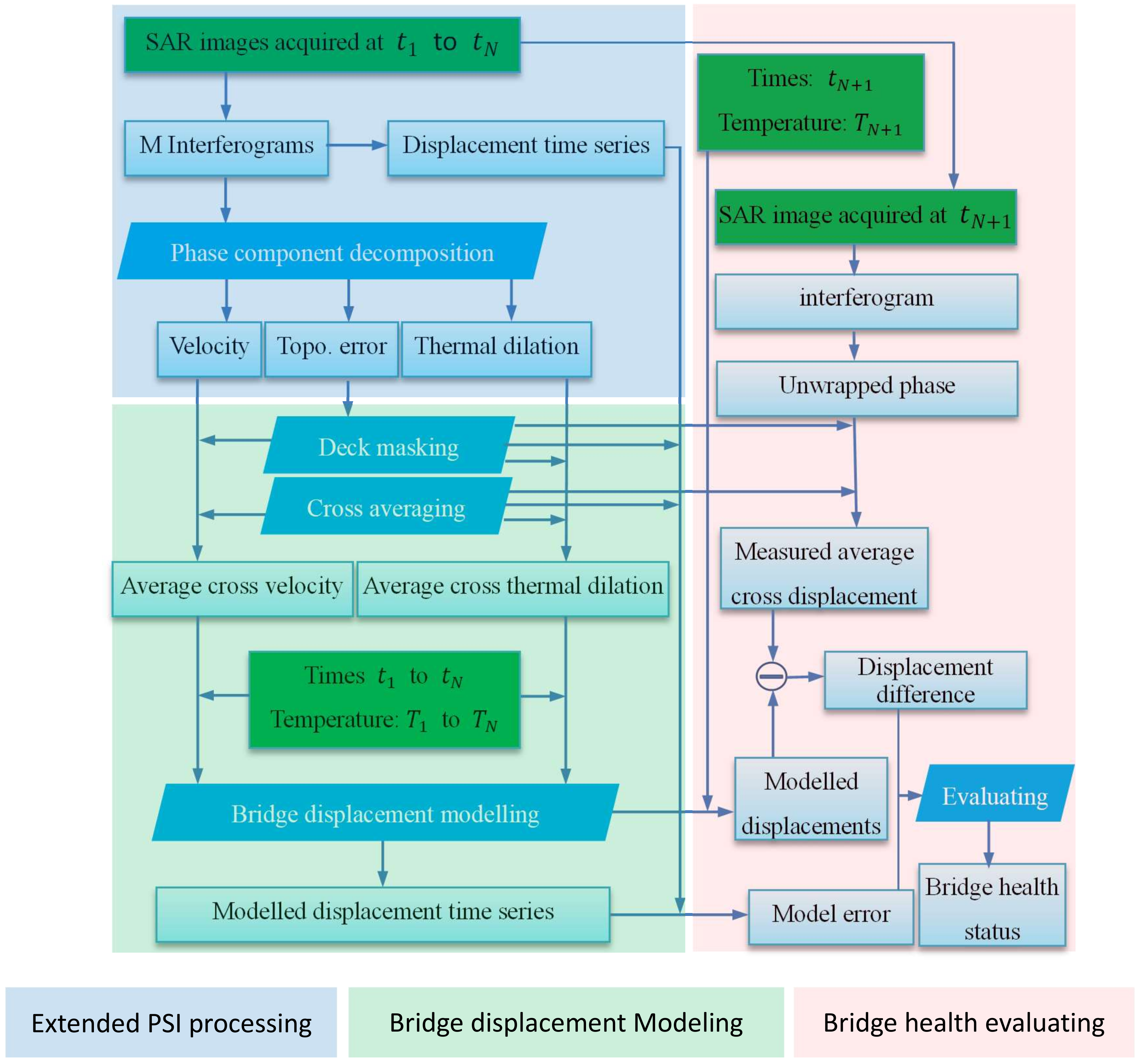
The key idea of the procedure is to: (i) use a set of SAR images to model the thermal dilation behavior of a given bridge; and then (ii) use additional SAR images to monitor the temporal evolution of the bridge. Figure 1 illustrates the flow chart of the procedure, which is composed of three parts highlighted in different colors. The procedure can be used to monitor the thermal dilation displacements of the entire bridge, exploiting the dense set of measurements provided by the PSI technique. The main steps of the procedure are described below.

• Collect $\mathrm{N}$ SAR images over the bridge of interest, acquired at times $t_1$ to $t_N$. Acquire, for each image, the temperature of the given scene at the time of acquisition of each image:$T_1$ to $T_N$.
• Generation of a redundant network of M interferograms from the N collected images (M >> N) [18], and calculation of the displacement time series using the traditional PSI method.

• The extended PSI model described in Reference [14] is used to estimate the main PSI phase components. This involves the following steps:

  (a)

  Pixel selection. In the SAR images, only those points characterized by low noise levels are selected using the amplitude dispersion index [19].

  (b)

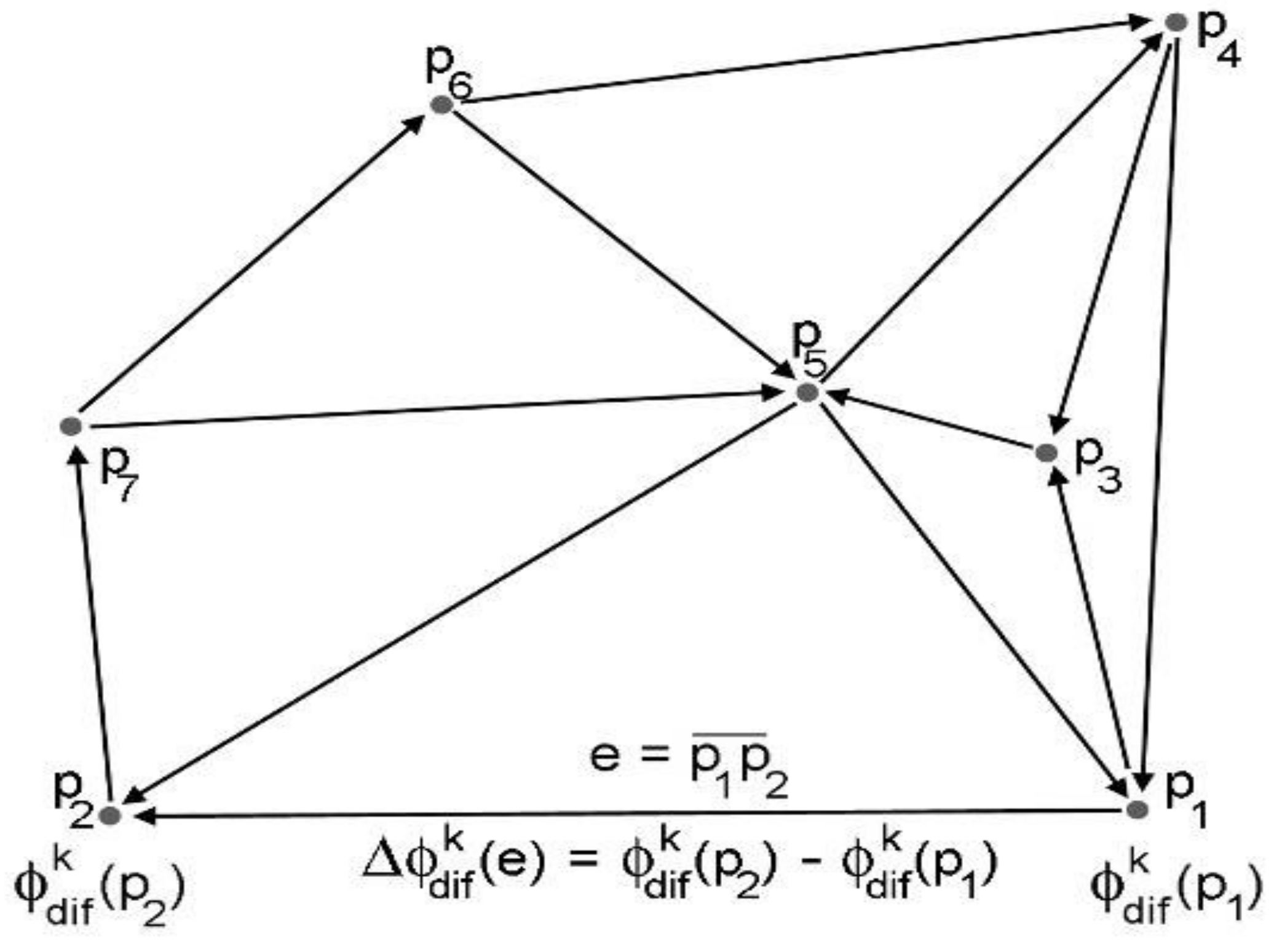
  Pixels connection. The selected pixels are connected by edges (Figure 2). For each interferogram $\mathrm{k}$ and edge $\mathrm{e}$, the phase difference $\Delta {\mathsf{\Phi }}^{\mathrm{k}}\left(\mathrm{e}\right)$ is derived. Let us call this difference $\Delta {\mathsf{\Phi }}_{\mathrm{obs}}^{\mathrm{k}}$.

  (c)

  Phase modeling and parameter estimation. For each phase difference, we can write:

  $$\Delta {\mathsf{\epsilon }}^{\mathrm{k}}=\Delta {\mathsf{\Phi }}_{\mathrm{obs}}^{\mathrm{k}}-\Delta {\mathsf{\Phi }}_{\mathrm{m}}^{\mathrm{k}}\left(\Delta \mathrm{v},\Delta \mathrm{te},\Delta \mathrm{Th}\right)$$

  (1)

  where $\Delta {\mathsf{\epsilon }}^{\mathrm{k}}$ is the differential phase residual associated with a given edge $\mathrm{e}$, while $\Delta {\mathsf{\Phi }}_{\mathrm{m}}^{\mathrm{k}}\left(\Delta \mathrm{v},\Delta \mathrm{te},\Delta \mathrm{Th}\right)=\frac{4\mathsf{\pi }}{\mathsf{\lambda }}\Delta {\mathrm{T}}^{\mathrm{k}}\Delta \mathrm{v}+\frac{4\mathsf{\pi }}{\mathsf{\lambda }}\frac{{\mathrm{B}}_{\perp }^{\mathrm{k}}}{{\mathrm{R}}^{\mathrm{k}}\sin \mathsf{\theta }}\Delta \mathrm{te}+\frac{4\mathsf{\pi }}{\mathsf{\lambda }}\Delta {\mathrm{Temp}}^{\mathrm{k}}\Delta \mathrm{Th}$ is the modeled differential phase. $\Delta \mathrm{v}$, $\Delta \mathrm{te}$ and $\Delta \mathrm{Th}$ are the differential unknowns associated with the edge $\mathrm{e}$; $\Delta \mathrm{v}$ is the differential deformation velocity; $\Delta \mathrm{te}$ is the differential topographic error; and $\Delta \mathrm{Th}$ is the so-called differential thermal dilation parameter; $\Delta {\mathrm{T}}^{\mathrm{k}}$ and ${\mathrm{B}}_{\perp }^{\mathrm{k}}$ are the temporal and perpendicular baseline of the interferogram k; $\Delta {\mathrm{Temp}}^{\mathrm{k}}$ is the temperature difference between the acquisitions of the two images of the interferogram $\mathrm{k}$; ${\mathrm{R}}^k$ and ${\mathsf{\theta }}^k$ are the slant range and incidence angle of the interferogram $\mathrm{k}$; and $\mathsf{\lambda }$ is the radar wavelength. To estimate the three unknowns for each edge $\mathrm{e}$, the following function is maximized numerically:

  $$\mathsf{\gamma }=\frac{1}{\mathrm{M}}{\displaystyle \sum }_{\mathrm{k}=1}^{\mathrm{M}}\exp \left(\mathrm{j}·(\Delta {\mathsf{\Phi }}_{\mathrm{obs}}^{\mathrm{k}}-\Delta {\mathsf{\Phi }}_{\mathrm{m}}^{\mathrm{k}}\left(\Delta \mathrm{v},\Delta \mathrm{te},\Delta \mathrm{Th}\right)\right)$$

  (2)

  where $\mathsf{\gamma }$ is a goodness of fit parameter, which indicates the quality of the estimation of the three unknowns; and $\mathrm{M}$ is the number of interferograms.

  (d)

  Phase component reconstruction. This step involves the integration of the differential unknowns $\Delta \mathrm{te}$, $\Delta \mathrm{v}$, and $\Delta \mathrm{Th}$. A minimum number of edges associated with a single pixel is set during the integration.

• Bridge displacement modeling and error estimation based on the estimated phase components. This involves the following steps:

  (a)

  Bridge deck masking. This step is based on the statistic result of the topographic errors achieved in step 3(d). Assuming the bridge deck is flat, a mask is built to select pixels on the bridge deck

  (b)

  Cross averaging. Instead of using the displacement measurements along the bridge longitudinal profile as in Refence [13], we average the above selected pixels in the cross-bridge direction. Therefore, robust and accurate displacement measurements along the longitudinal direction of the bridge are measured.

  (c)

  Bridge displacement modeling. Considering the cross averaged phase components on the bridge deck, the following displacement model can be established:

  $${\mathrm{d}}_{\mathrm{Long}}=\Delta \mathrm{Temp}·\Delta \mathrm{Th}+\Delta \mathrm{v}·\Delta \mathrm{t}$$

  (3)

  where ${\mathrm{d}}_{\mathrm{Long}}$ is the modeled longitudinal displacement, $\Delta \mathrm{Temp}$ and $\Delta \mathrm{t}$ are the temperature and temporal difference, respectively, and $\Delta \mathrm{Th}$ and $\Delta \mathrm{v}$ are the thermal dilation and linear velocity parameters along the bridge estimated by PSI.

  (d)

  Bridge displacement model error estimation. With the acquisition time ${\mathrm{t}}_1$ to ${\mathrm{t}}_{\mathrm{N}}$ and the temperature ${\mathrm{T}}_1$ to ${\mathrm{T}}_{\mathrm{N}}$, the model error, measured by the standard deviation of the differences between the cross-average value of the modeled displacements and the displacement time series achieved in step 2, is estimated.

• Bridge health evaluation. The idea for this evaluation is based on the hypothesis testing of the displacement differences, which are calculated between the upcoming measurements and the modeled ones, similar to Deviation Index DI1 described in Reference [20]. This includes the following two steps:

  (a)

  Differential displacement estimation. Let us assume that a new SAR image is acquired at ${\mathrm{t}}_{\mathrm{N}+1}$, with a temperature of ${\mathrm{T}}_{\mathrm{N}+1}$. Then, more interferograms are generated with the image ${\mathrm{t}}_{\mathrm{N}+1}$, and the cross-average displacements of the entire bridge deck are evaluated through interferogram phase unwrapping, bridge deck masking, and cross averaging. Such displacements are then compared with the modeled ones, and their difference is calculated:

  $${\mathrm{Diff}}_{\mathrm{Long}}^{\mathrm{k},\mathrm{k}+1}={\mathrm{Interf}}_{\mathrm{Long}}^{\mathrm{k},\mathrm{k}+1}-{\mathrm{Model}}_{\mathrm{Long}}^{\mathrm{k},\mathrm{k}+1}$$

  (4)

  where ${\mathrm{Model}}_{\mathrm{Long}}^{\mathrm{k},\mathrm{k}+1}=\Delta {\mathrm{Temp}}^{\mathrm{k},\mathrm{k}+1}·\Delta \mathrm{Th}+\Delta \mathrm{v}·\Delta {\mathrm{Tt}}^{\mathrm{k},\mathrm{k}+1}$ is the modeled longitudinal displacement, while ${\mathrm{Interf}}_{\mathrm{Long}}^{\mathrm{k},\mathrm{k}+1}$ is the measured one.

  (b)

  Bridge health evaluation. The differences between the measured and modeled displacements are assessed using the procedure described in Reference [13], and the confidence interval is given as twice the estimated model error. A positive evaluation is when the measured displacements are within the confidence interval (i.e., the bridge shows a good behavior, or the displacements are within the design parameters of the bridge). Otherwise, a detailed analysis of the bridge, and especially of the bearings, is required.

3. Description of the Test Sites and Datasets

3.1. The NDHRB

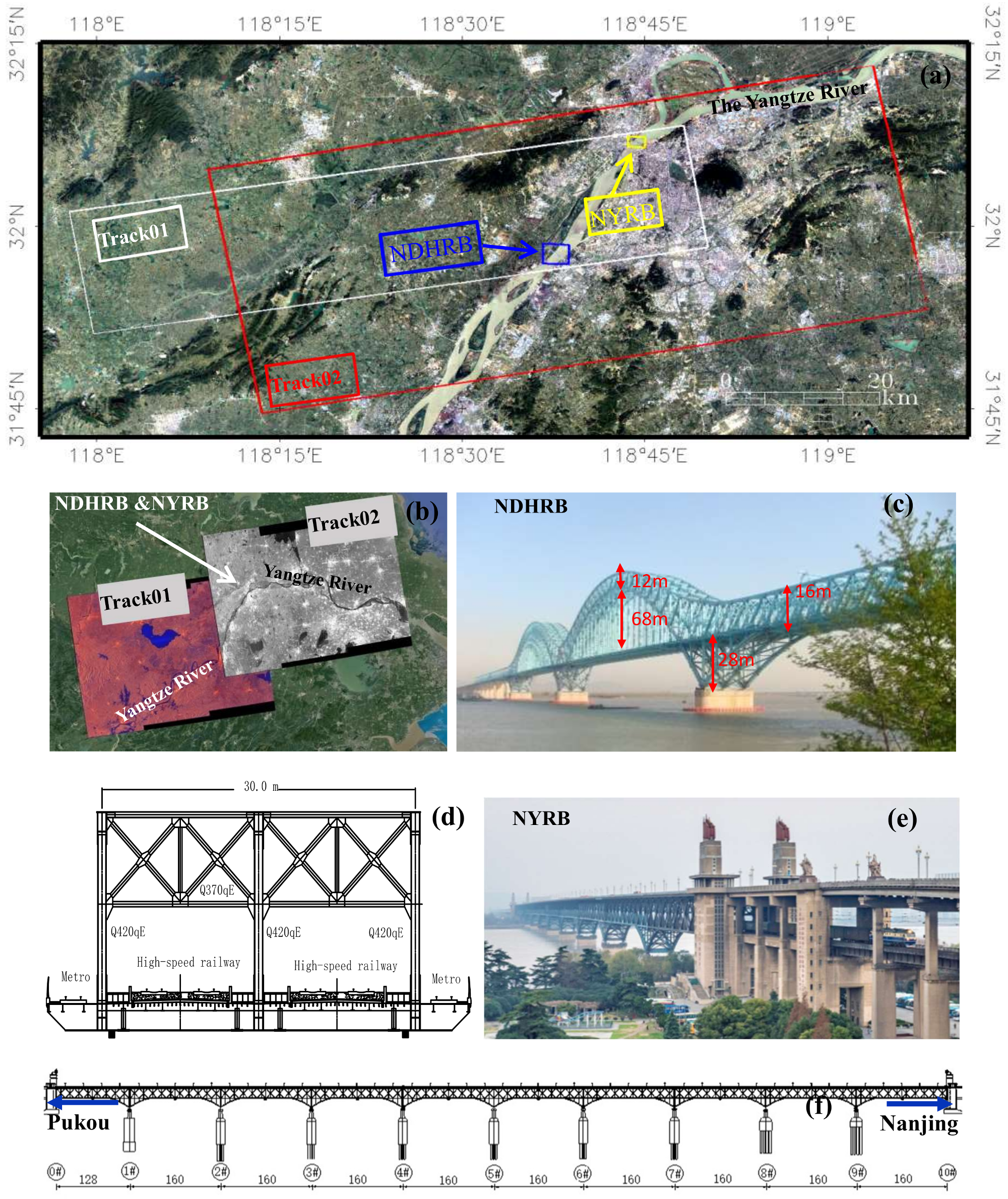
Nanjing-Dashengguan High-speed Railway Bridge (NDHRB) is located in the Nanjing section of the middle and lower reaches of the Yangtze River, in China. This bridge (see the blue rectangle in Figure 3a) is the world’s longest span high-speed railway bridge and the largest bridge with the heaviest design load ever built [17]. The structure of the NDHRB includes an orthogonal steel deck system; the heights of each part are highlighted in Figure 3c. The bridge includes six tracks: two tracks of the Beijing-Shanghai high-speed line; two tracks of the Shanghai-Chengdu railway lines; and two tracks of the Nanjing Metro. For more details, see Reference [17]. The bridge is supported by six sliding bearings (4#, 5#, 6#, 8#, 9#, 10#) on the two sides of the bridge and a fixed bearing (7#) located in the center of the bridge. The deck cross-section of NDHRB is shown in Figure 1d. The main structure of the bridge was built using three types of steel: Q345qD, Q370qE, and Q420qE. Their coefficients of thermal expansion (CTE) are 16.0 × 10⁻⁶/°C, 13.0 × 10⁻⁶/°C, and 13.0 × 10⁻⁶/°C, respectively.

3.2. The NYRB

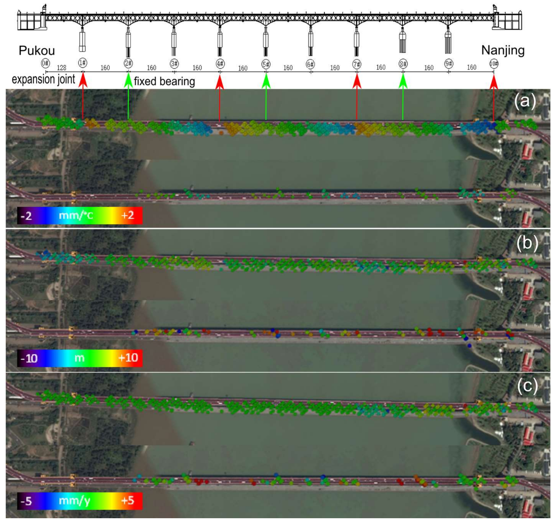
Nanjing-Yangtze River Bridge (NYRB) (the yellow rectangle in Figure 3a), connects the Beijing-Shanghai railway and the Nanjing-Yangzhou national highway. It is the first highway-cum-railway bridge (the upper layer is a highway, and the lower layer is a railway) built in China. It was opened on 29 December 1968, after ten years of construction. The main bridge is 1576-m long (128 m, plus 160 m by 9): it includes a simply-supported steel truss girder, with a span of 128 m, and 9 remaining continuous steel truss girders of 160 m, where every three spans are united as a bridge segment (span-continuous truss) [21]. In order to adapt to the longitudinal displacement of the bridge decks caused by temperature changes, huge expansion joints are mounted between the three segments at 1#, 4#, 7#, and 10# piers, with a maximum moving ability of 38 cm for 1#, 55 cm for 4# and 7#, and 34 cm for 10# [22]. Movable bearings are mounted at 1#, 3#, 4#, 6#, 7#, 9#, and 10#, while fixed bearings are on 0#, 2#, 5#, and 8#. Low alloy steel of 16Mnq is used as the main structure of the main girder and railway cross-section [23], with a CTE of 11.26 × 10⁻⁶/°C. The overall layout of the NYRB is shown in Figure 3f. It should be noted that the bridge was closed for 27 months for comprehensive repair and maintenance work at the end of 2016.

3.3. The Sentinel-1 Datasets

The two bridges are imaged in the overlap area of two ascending Sentinel-1 tracks: track 01 (the absolute orbit number of the first image, acquired on 25 April 2015, is 005639); and track 02 (the absolute orbit number of the first image, acquired on 2 April 2015, is 005437): see Figure 3b. Specifically, this occurs in a single burst of the third swath of track 01 (see the white rectangle in Figure 3a), and two bursts of the first swath of track 02 (see the red rectangle in Figure 3a). Seventy-five IW mode SAR images, acquired between 25 April 2015 and 15 May 2018, are available for track 01. Track 02 has sixty-six IW mode SAR images, acquired between 8 April 2015 and 10 May 2018; the SAR image datasets of track 01 and track 02 are listed in

Table 1. Sentinel-1 SAR image dataset of Track 01 (the non-bold group is used for displacement modeling and the bold one for health evaluation).

No.	Date	T/°C	No.	Date	T/°C	No.	Date	T/°C	No.	Date	T/°C	No.	Date	T/°C
1	20150425	25.0	16	20160126	4.8	31	20160829	27.2	46	20170414	24.7	61	20171104	11.7
2	20150706	18.2	17	20160219	12.6	32	20161004	22.4	47	20170426	17.8	62	20171116	14.1
3	20150730	33.0	18	20160302	16.6	33	20161016	20.7	48	20170508	15.6	63	20171128	14.4
4	20150811	27.5	19	20160314	11.8	34	20161028	12.8	49	20170520	28.6	64	20171210	8.4
5	20150823	27.5	20	20160326	11.3	35	20161109	10.3	50	20170601	32.5	65	20171222	11.5
6	20150916	25.2	21	20160407	17.8	36	20161203	11.5	51	20170613	22.4	66	20180103	1.8
7	20150928	26.3	22	20160419	21.0	37	20161215	4.4	52	20170625	28.5	67	20180115	11.6
8	20151010	19.6	23	20160501	26.8	38	20161227	2.8	53	20170719	34.1	68	20180127	−1.2
9	20151022	22.6	24	20160513	18.4	39	20170108	5.7	54	20170731	33.8	69	20180220	4.2
10	20151103	15.8	25	20160525	27.7	40	20170201	3.7	55	20170812	26.2	70	20180304	16.4
11	20151115	17.1	26	20160606	24.9	41	20170213	12.6	56	20170824	32.1	71	20180328	24.6
12	20151127	4.5	27	20160630	30.7	42	20170225	11.0	57	20170905	26.7	72	20180409	23.3
13	20151209	10.3	28	20160724	36.3	43	20170309	16.1	58	20170917	27.0	73	20180421	22.5
14	20151221	7.0	29	20160805	29.7	44	20170321	13.2	59	20171011	15.1	74	20180503	24.1
15	20160114	3.6	30	20160817	33.0	45	20170402	19.6	60	20171023	15.1	75	20180515	33.2

and

Table 2. Sentinel-1 SAR image dataset of Track 02 (the non-bold group is used for displacement modeling and the bold one for health evaluation).

No.	Date	T/°C	No.	Date	T/°C	No.	Date	T/°C	No.	Date	T/°C	No.	Date	T/°C
1	20150408	10.8	16	20160601	20.2	31	20170304	16.4	46	20170912	26.6	61	20180311	18.6
2	20150502	17.9	17	20160719	30.3	32	20170316	11.9	47	20170924	21.4	62	20180323	18.5
3	20150701	27.8	18	20160812	33.7	33	20170328	19.5	48	20171006	19.1	63	20180404	11.9
4	20150725	28.5	19	20160929	18.3	34	20170409	11.8	49	20171018	15.9	64	20180416	16.9
5	20150818	28.4	20	20161011	18.2	35	20170421	20.4	50	20171030	12.5	65	20180428	25.1
6	20150911	25.1	21	20161023	16.2	36	20170503	21.1	51	20171111	13.9	66	20180510	20.8
7	20151005	20.4	22	20161104	16.9	37	20170515	20.2	52	20171123	11.2	67
8	20151122	16.6	23	20161116	14.9	38	20170527	30.6	53	20171205	5.7	68
9	20151216	4.3	24	20161128	9.5	39	20170608	28.4	54	20171217	1.9	69
10	20160109	8.1	25	20161210	10.3	40	20170702	24.3	55	20171229	10.5	70
11	20160202	2.5	26	20170103	11.2	41	20170714	33.8	56	20180110	2.8	71
12	20160226	15.3	27	20170115	4.0	42	20170726	36.2	57	20180122	8.1	72
13	20160321	15.0	28	20170127	6.5	43	20170807	32.2	58	20180203	-1.2	73
14	20160414	24.2	29	20170208	1.0	44	20170819	30.1	59	20180215	6.6	74
15	20160508	14.2	30	20170220	4.4	45	20170831	20.0	60	20180227	14.3	75

, and the ambient temperatures were acquired from the Pukou weather station, respectively. Due to the different swaths of the two tracks, the corresponding incidence angles are 45° for track 01, and 31° for track 02.

4. Feasibility Study: SAR Measurement Sensitivity

This section presents a sensitivity analysis of the longitudinal deformations of the SAR-based measurements for both datasets. The aim of this study is to calculate the sensitivity parameter and evaluate the feasibility of the proposed PSI-based approach. For details on the sensitivity analysis of the line of sight (LOS) observation regarding the different sensors, see Reference [25].

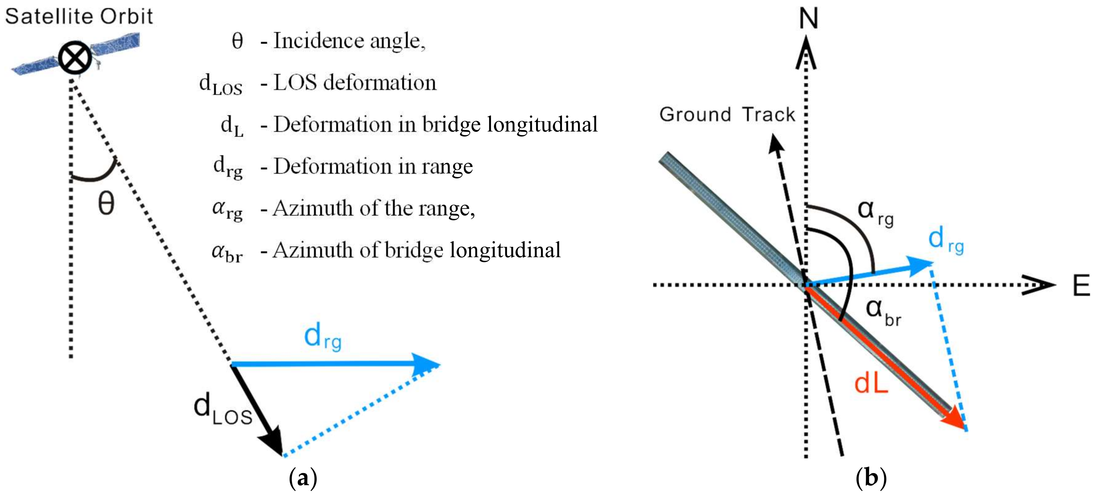
Due to the Line-of-Sight (LOS) nature of the displacements measured using SAR interferometry, the structural displacement monitoring capability depends on the SAR geometry and the azimuth of the bridge’s main axis. We assumed that the most important contribution of the temperature related movements was longitudinal [13]. Thus, considering only the displacements in the longitudinal direction, the relation between the LOS and the longitudinal deformation can be written as follows (see Figure 4):

$${\mathrm{d}}_{\mathrm{L}}=\frac{{\mathrm{d}}_{\mathrm{LOS}}}{\sin \mathsf{\theta }\cos \left({\mathsf{\alpha }}_{\mathrm{br}}-{\mathsf{\alpha }}_{\mathrm{rg}}\right)}$$

(5)

where ${\mathrm{d}}_{\mathrm{LOS}}$ and ${\mathrm{d}}_{\mathrm{L}}$ are the LOS and longitudinal deformation, respectively; $\mathsf{\theta }$ is the incidence angle, and $\mathsf{\alpha }={\mathsf{\alpha }}_{\mathrm{br}}-{\mathsf{\alpha }}_{\mathrm{rg}}$ is the horizontal angle given by the difference of the SAR range azimuth, ${\mathsf{\alpha }}_{\mathrm{rg}}$, and bridge longitudinal azimuth, ${\mathsf{\alpha }}_{\mathrm{br}}$.

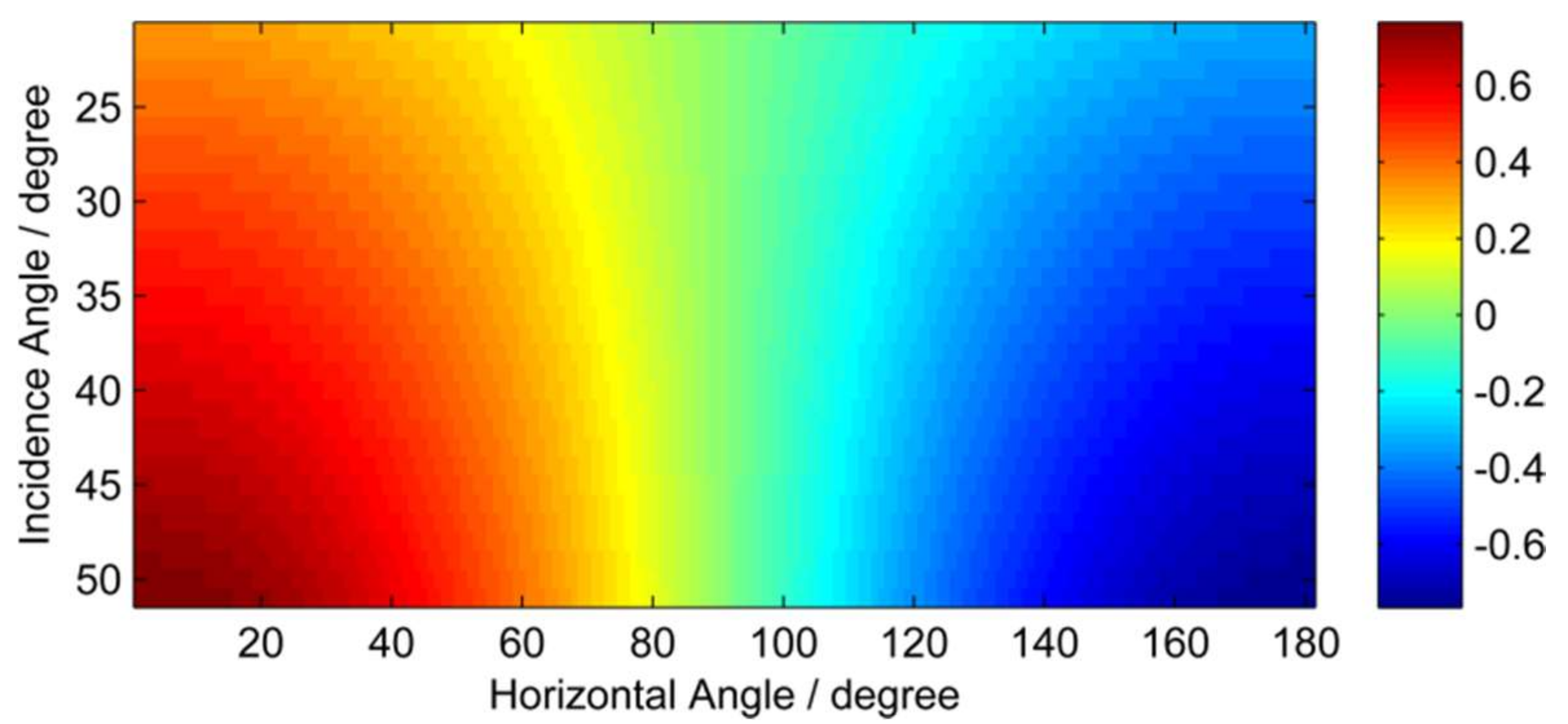
Let us define $\mathrm{s}=\sin \mathsf{\theta }\cos \mathsf{\alpha }$ as the sensitivity of the longitudinal displacements of bridge in the LOS. The larger the s is, the better the measurements are. Figure 5 illustrates the relationship between $\mathrm{s}$, the radar incidence angle $\mathsf{\theta }$, and the horizontal angle $\mathsf{\alpha }$. When the SAR range direction is perpendicular to the bridge’s main axis, the sensitivity goes to zero and the longitudinal displacements cannot be measured. The sensitivity of the NDHRB and the NYRB, calculated with the geometry of Track 01 and Track 02, is listed in

Table 3. Sensitivity to the longitudinal displacements of the NDHRB and the NYRB, computed with the geometry of Track 01 and Track 02.

	NDHRB		NYRB
	Track 01	Track 02	Track 01	Track 02
$\mathsf{\theta }$/degree	45.0	31.0	45.0	31.0
${\alpha }_{\mathrm{br}}$/degree	133.6	133.6	120.6	120.6
${\alpha }_{\mathrm{rg}}$/degree	79.5	79.5	79.5	79.5
$\mathsf{\alpha }$/degree	54.1	54.1	41.1	41.1
$\mathrm{s}$	0.41	0.30	0.53	0.39

.

5. PSI Processing

To evaluate bridge health using the method presented in Section 2, we divided each dataset into two groups (distinguished by bold and non-bold fonts in Table 1 and Table 2): the first group (non-bold) was used for modeling the bridge displacement, while the second group (bold) was used for evaluating bridge health.

Software developed by CTTC was used for SAR data processing [26]. It consists of two main parts: the generation of differential interferograms; and the modeling and decomposition of phase components.

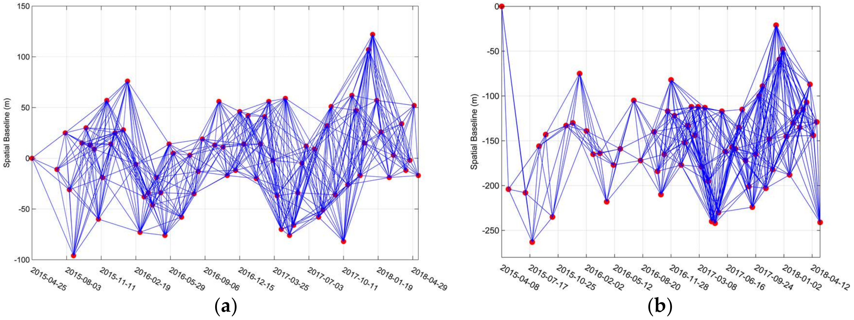
A redundant network was used for the phase component decomposition. All interferograms with temporal baselines of less than 132 days were generated (see Figure 6). A 3-arc SRTM DEM was used for topographic phase removing. In total, 585 interferograms were generated for Track 01 and 485 for Track 02. The maximum spatial baseline for Track 01 was 196 m (interferometric pair 20171011_20180103) and 263 m for Track 02 (interferometric pair 20150408_20150725). The minimum spatial baselines for the two tracks were 2 m (interferometric pair 20161227_20170213) and 1 m (interferometric pair 20170702_20170714), respectively. The SAR multi-looking was not applied to preserve the original resolution of the data.

The amplitude dispersion index (DA) was applied for pixel selection. The threshold was set to 0.2. Edges with γ < 0.7 were discarded, and a minimum number of 10 edges associated with a single point was set for the integration. Finally, the three-phase components (linear velocity, topographic error, and thermal dilation coefficient) were extracted numerically with the extended PSI model [14].

6. PSI Results

6.1. NDHRB

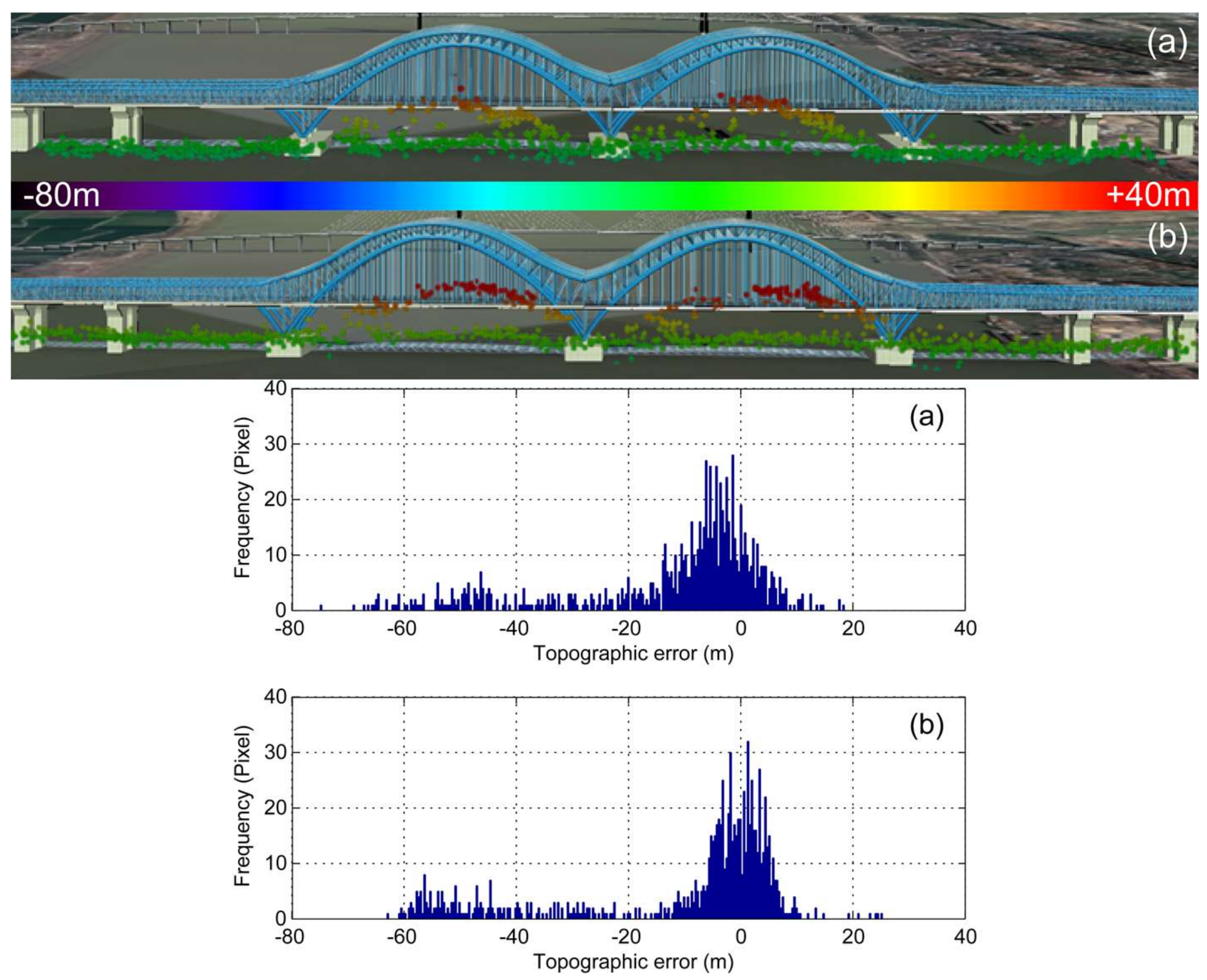
The topographic error is given by the difference between the Digital Terrain Model (DTM) used in the interferogram generation and the actual height of a given scatterer. Figure 7 shows the topographic error and its statistics using the two tracks: the two arcs of the bridge can be clearly identified. The distribution of the topographic error is similar in both cases: as seen below, both include a uniform distribution, which corresponds to the bridge arcs, and a normal distribution, which is related to the other part of the bridge.

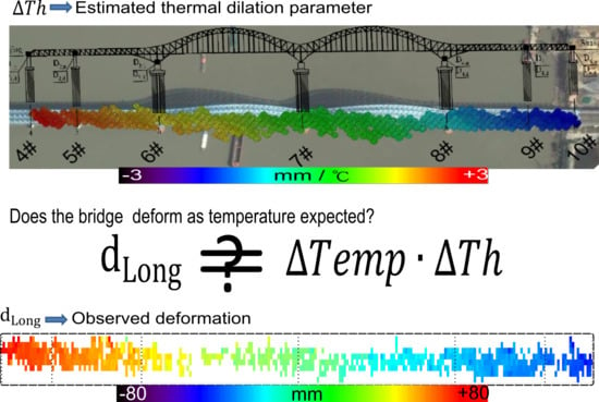
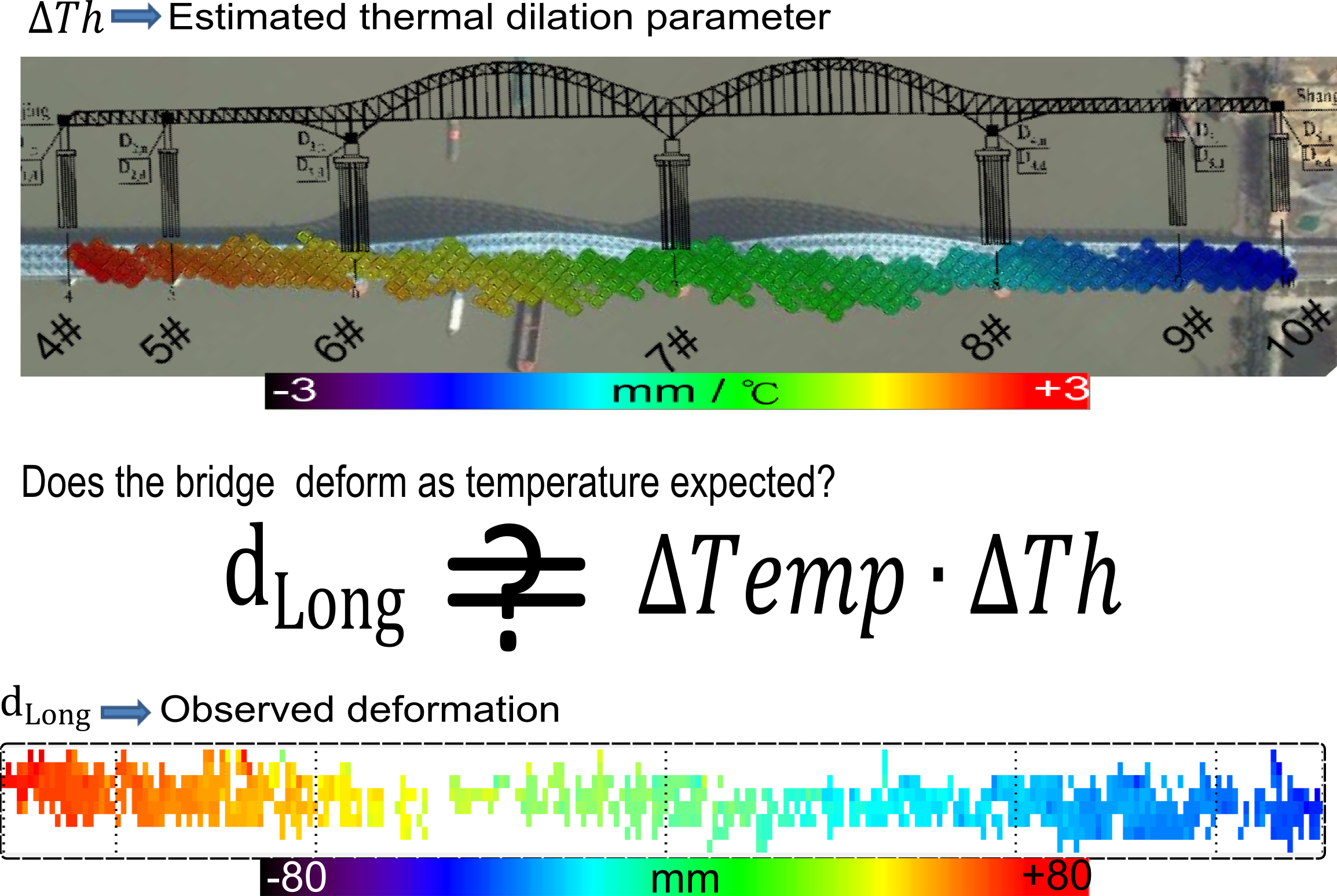
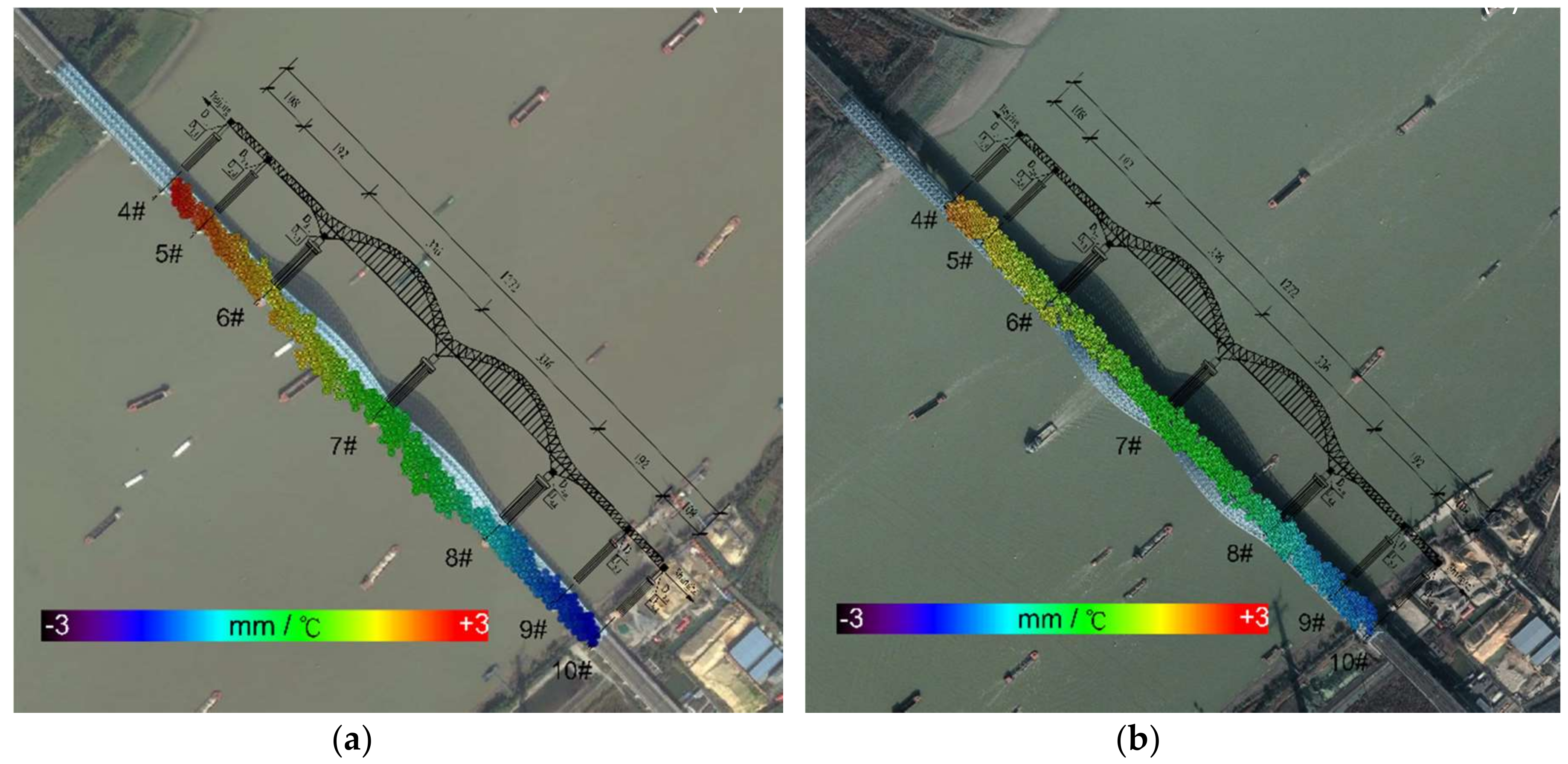
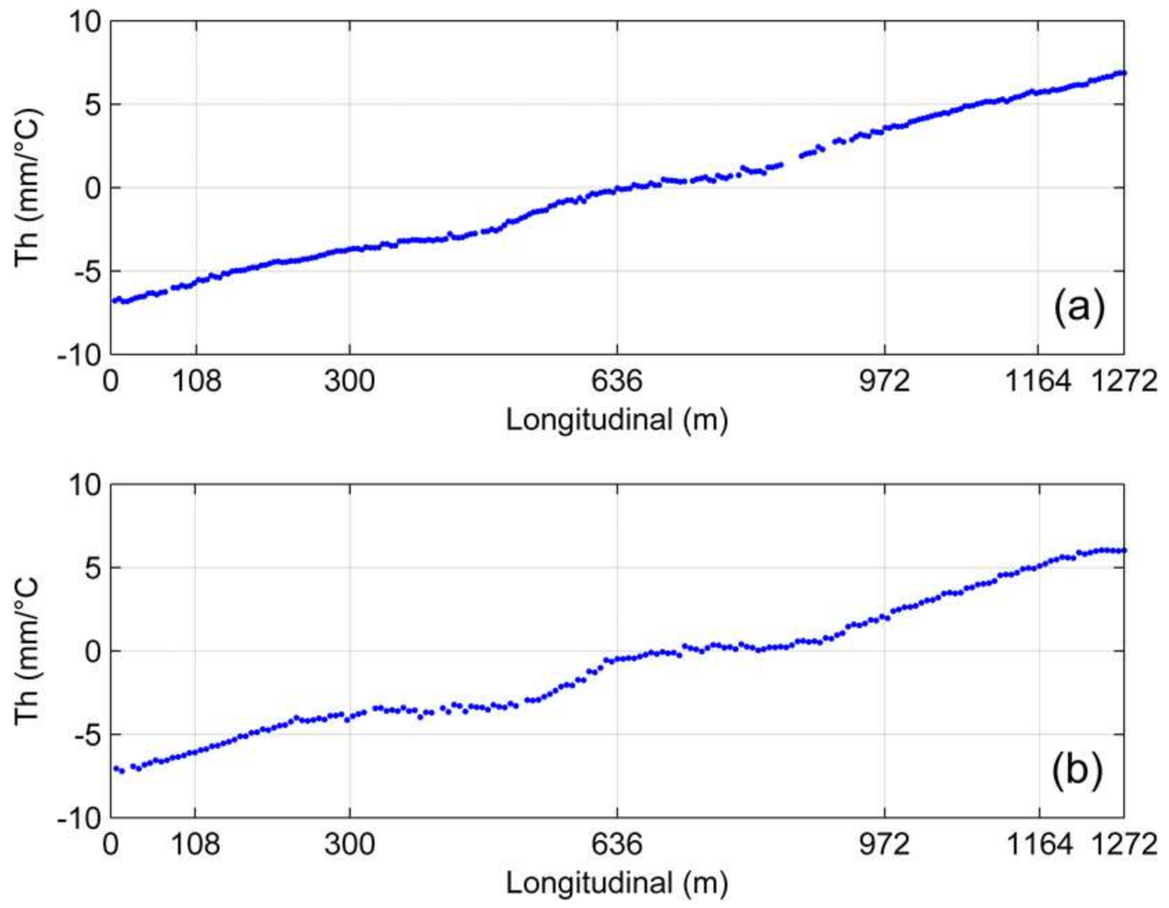
To study the displacements of the bridge deck, a mask was applied to the map of the thermal dilation parameter and linear velocity: only those points whose heights are between −10 m and 10 m were selected. This was followed by the projection of the LOS displacements into the longitudinal bridge direction. Figure 8 shows the estimated thermal dilation parameters in the LOS direction; Figure 9 presents their average cross values in the longitudinal direction for the two tracks, while Figure 10 shows the average cross values of the LOS linear velocities for the two tracks. The main results related to thermal dilation are summarized in

Table 4. Thermal dilation parameters of the NDHRB.

	Track 01	Track 02
PS/pixels	903	942
${\mathrm{d}}_{\mathrm{LOS},\mathrm{Max}}$(mm/)	3.06	2.31
${\mathrm{d}}_{\mathrm{LOS},\mathrm{Min}}$ (mm/°C)	−2.88	−2.00
${\mathrm{d}}_{\mathrm{LOS},\mathrm{total}}$ (mm/°C)	5.94	4.31
${\mathrm{d}}_{\mathrm{L},\mathrm{total}}$ (mm/°C)	14.33	14.24
CTE (/°C)	11.26 × 10−6	11.19 × 10−6

. This is discussed in the following four sections.

(1) A large number of Persistent Scatterer (PS) measurements were obtained on the deck of the NDHRB, for both Track 01 (903) and Track 02 (942). They are uniformly distributed, covering the entire bridge. Many PSs are from the steel truss girder and the bridge deck, including railway sleepers, tracks, and ballast. The change in the incidence angle of the radar has very little impact on the scattering characteristics of NDHRB.

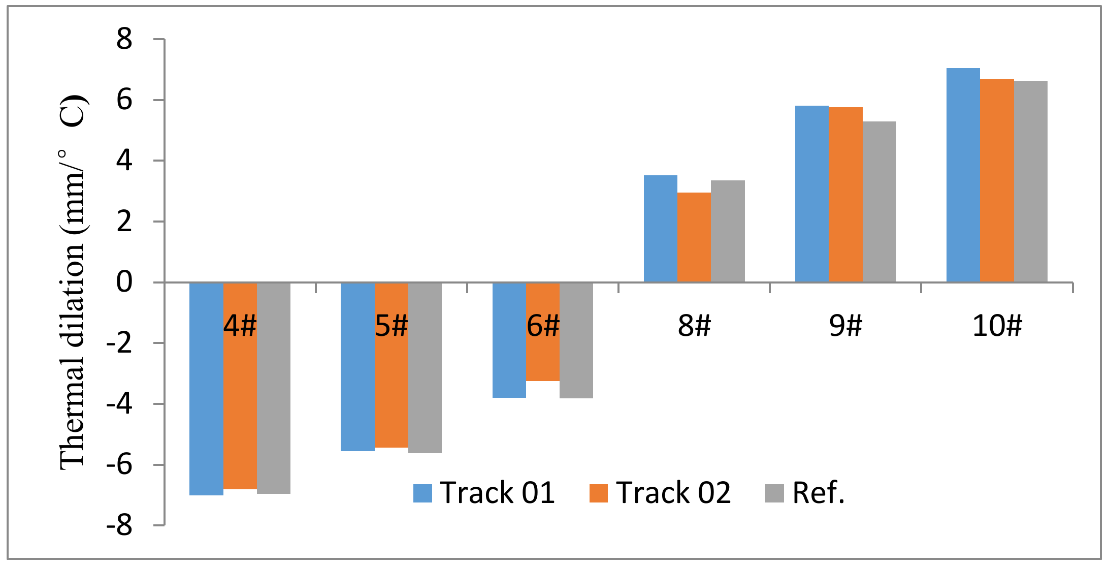
(2) Similar thermal dilation characteristics were observed on the two tracks. Results show that the thermal dilation parameters on both sides of the bridge are almost equal but with opposite signs. The magnitude of the thermal dilation parameter increases with the distance from the bridge center, where the fixed bearing (7#) is located. The measured CTE (11.26 × 10⁻⁶ and 11.19 × 10⁻⁶ for Tracks 01 and 02, respectively) match the bridge properties mentioned in Section 1, and the results described in Reference [13]. To validate the accuracy of the thermal dilations measured using PSI, the thermal dilations observed at the six movable bearings and the in-situ measurements [17] were compared (see Figure 11). Taking the in-situ measurements as Reference, the absolute mean error is 0.25 mm/°C.

(3) The average cross values of the linear velocity calculated for the LOS displacement for both tracks are below 2 mm/year, and there is no clear correlation between the two tracks. Comparing this estimated linear deformation with the displacement caused by the thermal dilation: the relative thermal dilation parameters of the entire bridge, in the LOS, reached 5.94 mm/°C and 4.31 mm/°C (see Table 4), this means that a temperature variation of 30 °C causes at least 130 mm of LOS displacement; hence the estimated linear deformation is much smaller. The velocity values shown in Figure 10 could be due to residual non-modeled thermal dilation displacements, and can be neglected in bridge displacement modeling.

(4) Table 4 shows the thermal dilation parameters estimated using Track 01 and Track 02: the difference in the total longitudinal parameter (${\mathrm{d}}_{\mathrm{L},\mathrm{total}}$) of the two tracks is 0.09 mm/°C, which corresponds to 2.7 mm with a temperature variation of 30 °C. These results depict the high sensitivity of the proposed approach.

(5) Considering the length of the NDHRB (1272 m), the CTE of the NDHRB can be estimated, corresponding to 11.26 × 10⁻⁶/°C and 11.19 × 10⁻⁶/°C for the two tracks: they agree well with each other (see Table 4). The differences between these values and 13.0 × 10⁻⁶/°C, which is the CTE of Q420qE that dominates the expansion of the bridge, are 1.74 × 10⁻⁶/°C and 1.81 × 10⁻⁶/°C: their relative errors are 13% and 14%. The relatively smaller observed CTE values can be explained by the friction of movable bearings.

6.2. Results of NYRB

Due to the comprehensive maintenance of the NYRB, the interferometric coherence decreases dramatically for all SAR acquisitions; hence, only 45 images in Track 01 and 34 images in Track 02, from their first acquisitions, were used for PSI processing.

Figure 12 shows the LOS phase components of the NYRB estimated with Track 01 (upper) and Track 02 (lower). It is very clear that the PS density is quite different: Track 01 has far more measurements (640) than Track 02 (96). Hence, with more PS measurements covering the entire bridge, Track 01 is capable of providing valuable phase information, while Track 02 fails. The diversity of the PS density can be explained by the fact that the upper layer of the NYRB is a highway that is relatively flat for C-band radar signal, while the lower part of the bridge, constructed with metal truss, has strong backscattering. With the decrease in the radar incidence angle, the upper layer with less backscattering becomes the main scattering area, hence, the amount of PSs decreases dramatically.

Three segments of the NYRB are highlighted by the thermal dilation coefficients in Figure 12a, which corresponds with the architectural properties of the bridge (four fixed bearings mounted at 0#, 2#, 5#, and 8#, see the green arrows, and huge expansion joints mounted at 1#, 4#, 7#, and 10#, see the red arrows in Figure 12). On each segment, the thermal dilation is zero in the fixed pier, and the values increase towards each side up to the expansion joints, but with opposite signs. The thermal dilation parameters of the NYRB at the middle segment (480 m) are listed in

Table 5. Thermal dilation parameters of the NYRB at the middle segment.

	Track 01	Track 02
PS/pixels	640	96
${\mathrm{d}}_{\mathrm{LOS},\mathrm{Max}}$ (mm/°C)	1.23	-
${\mathrm{d}}_{\mathrm{LOS},\mathrm{Min}}$ (mm/°C)	1.43	-
${\mathrm{d}}_{\mathrm{LOS},\mathrm{total}}$ (mm/°C)	2.66	-
${\mathrm{d}}_{\mathrm{L},\mathrm{total}}$ (mm/°C)	5.02	-
CTE (/°C)	10.46 × 10−6	-

. It can be seen that the difference in the estimated CTE and the structural property is very small (0.80 × 10⁻⁶/°C), corresponding to a relative error of 7.1%. The under-estimated value can be explained by the small internal stresses of the structure. The absolute values of the estimated topographic errors are all less than 10 m (see Figure 12b), which also correspond well with the flat characteristics of the NYRB. The estimated linear deformation rates shown in Figure 12c are mostly around 0 mm/year, which shows that the NYRB had no linear deformation during the monitoring period.

7. Bridge Health Evaluation

We assumed that the bridges were in a healthy state during the SAR monitoring period in the first group. By considering the NDHRB as an example, the two datasets were used independently to evaluate the bridge health using the procedure presented in Section 2. The bridge states of the two acquisitions from each track in the second group—that is, 3 May and 15 May 2018 for Track 01, and 28 April and 22 May 2018 for Track 02—were evaluated. The longitudinal displacement measurements of the bridge obtained from unwrapped interferograms were compared with the modeled ones, and the differences were used for the hypothesis testing. Hence, the health of the bridges was evaluated on the final SAR imaging dates.

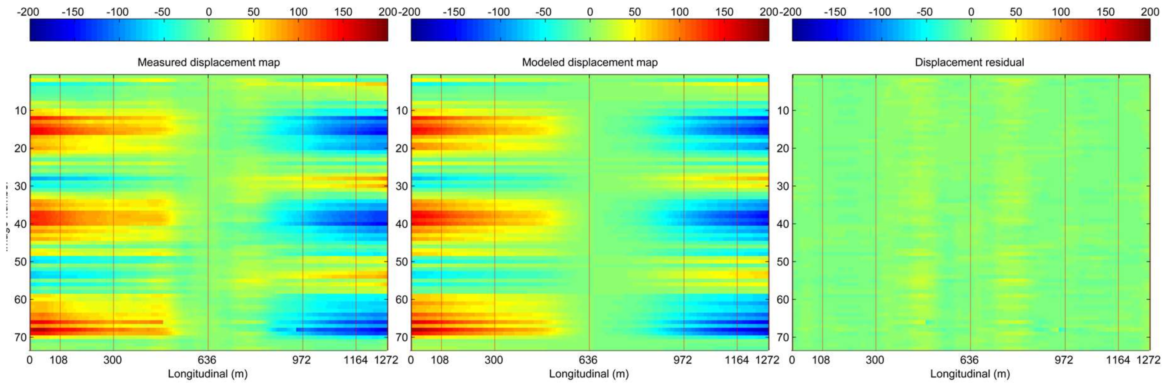
The accuracy of the structural displacement model was estimated by evaluating the difference between the modeled and observed displacement time series during the designed stable life period of the bridge. Figure 13 shows the measured displacement time series, the modeled displacement time series, and their difference for Track 01 over the NDHRB; the standard deviation of their difference is 5.9 mm, while the value for Track 02 is 6.2 mm. It should be noted that the linear term of the displacement residual in each acquisition was estimated and removed.

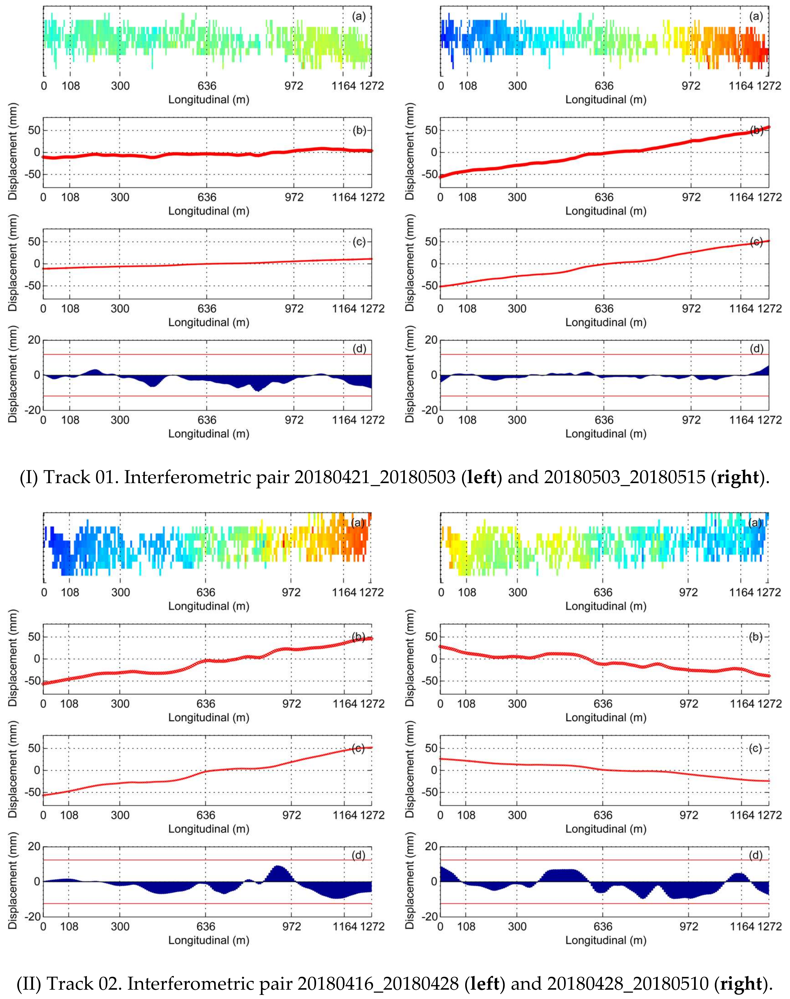
Figure 14 shows the NDHRB health evaluation results using the proposed procedure in four SAR image acquisitions: 20180503, 20180515, 20180428, and 20180510. In each evaluation procedure, Figure 14 with ‘(a)’ is the unwrapped interferogram, ‘(b)’ is the measured average cross displacement, ‘(c)’ is the modeled displacements, and ‘(d)’ is the displacements difference between the measured and modeled value. The atmospheric effects are neglected assuming that the area is small enough to avoid significant contributions. Moreover, in order to ease the phase unwrapping, only the points located on the bridge deck are used. Considering two times the absolute mean error of the models (2 × 5.9 mm = 11.8 mm for Track 01, and 2 × 6.2 mm = 12.4 mm form Track 02), the up control line (UCL) and the lower control line (LCL) can be drawn at ±11.8 mm and 12.4 mm, respectively (see the red lines in ‘(d)’ of Figure 14). It can be seen that all of the displacement differences are included in the control lines, while some large values are mainly caused by traffic along the bridge, e.g., pair 20180428_20180510. Therefore, in this case, there are no abnormal displacements of the entire bridge in the four periods observed.

8. Discussion

Displacement monitoring plays an important role in structural health evaluation. In this study, displacement monitoring and health evaluation of two bridges (the NDHRB and the NYRB) using the PSI technique and SAR interferometry were carried out.

We analyzed the sensitivity of Sentinel-1 space-borne SAR interferometry to measure structural displacements. The approach used can be replicated in different bridges to select the best track and frame before beginning the download of the images.

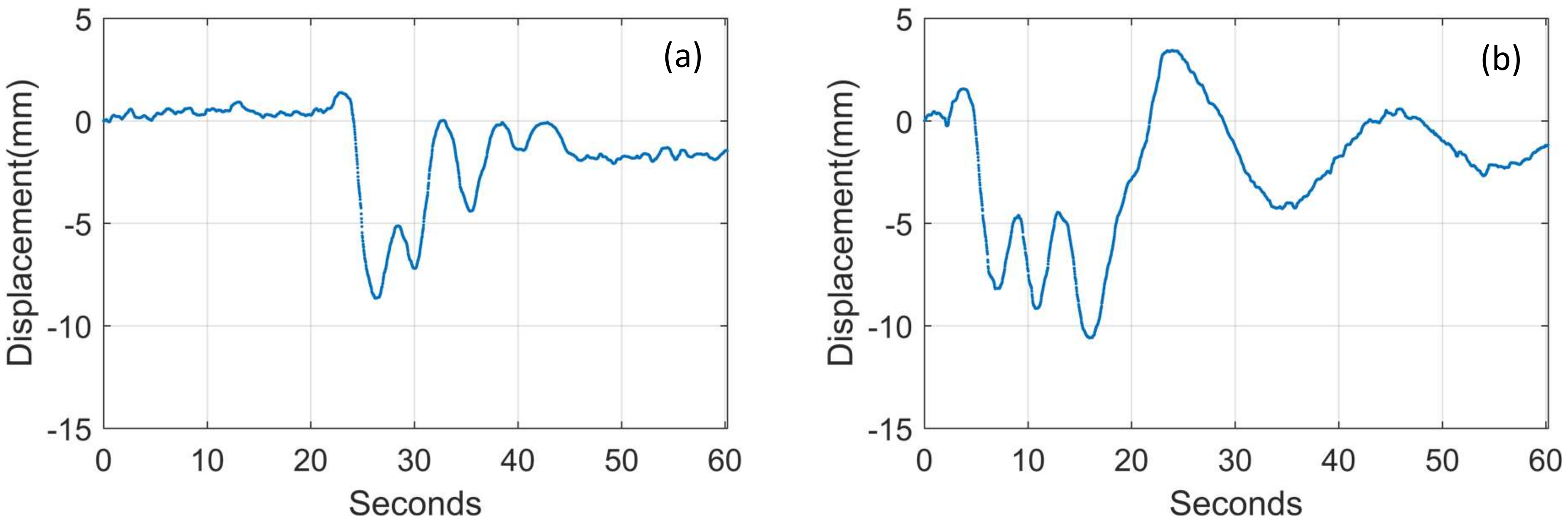
The results obtained have demonstrated the applicability of the proposed approach on two bridges with very different structural characteristics. The estimated sensitivity to anomalous displacements in the proposed health evaluation approach was around 1 cm. Such precision is good enough for a wide range of bridges. In this context, Figure 15 shows two temporal profiles of the movement of a point located at the middle of the bridge (192 m-span) and measured through an in-situ real aperture radar [27]. These time series show the vertical displacement of the point induced by a high-speed train (a) and a metro (b). It can be seen that all the induced displacements are below the centimeter.

A total of 903 and 942 points were measured on the NDHRB using two Sentinel-1 tracks: such measurements made it possible to monitor the displacements of the entire bridge. Moreover, the use of two independent tracks in this bridge provided a cross-validation of the results obtained, which was useful for assessing the precision of the methods used. The number of PS measurements on the NYRB decreased dramatically as the radar incidence angle decreased from 45 degrees (in the third swath) to 31 degrees (in the first swath). In this case, it was only possible to obtain results with one trajectory.

Using two tracks of Sentinel-1 SAR images (75 and 76 images, respectively) was useful for assessing the results obtained from two independent datasets. However, the results obtained from both datasets could also be merged to provide higher temporal sampling for the SHM. During the period observed, the bridges underwent no actual displacements. Hence, the thermal dilation displacements were dominant. The total thermal dilation parameters of the NDHRB, estimated using the two datasets, were compared. A discrepancy of 0.09 mm/°C was found, which corresponds to a difference of 2.7 mm over the total length of the bridge, assuming a temperature variation of 30 °C. The total thermal dilation parameter was 14.28 mm/°C, which resulted in a CTE of 11.22 × 10⁻⁶/°C: this corresponds well with material properties of the bridge. Similar results were obtained from the NYRB.

Finally, it is worth underlining that such an approach cannot be applied to all bridges due to different issues such as SAR geometry limitations, traffic along the bridge, or structural characteristics. However, depending on the location of the area of interest, the acquisition policy of Sentinel-1 constellation could help to minimize such limitations by offering the possibility of acquiring ascending and descending data, and, in some cases, of working with parallel adjacent tracks, as in the case of the two bridges analyzed. Moreover, the continuous acquisition mode providing an image every 6, 12, or 24 days, depending on the location, makes it possible to devise long-term monitoring plans.

9. Conclusions

In this paper, a procedure for continuously assessing the displacements of a bridge has been proposed. It has been successfully applied on two huge bridges—the NDHRB and the NYRB—by using medium-resolution Sentinel-1 SAR images. The results have been cross-validated by using two independent datasets obtaining millimeter-order differences. A bridge health evaluation method, based on longitudinal displacements covering the entire bridge deck, has been presented and validated on the NDHRB. This method evaluates the abnormal displacements along the entire bridge deck, which is an advantage with respect to methods that only measure the displacements with respect to the piers. Its applicability has been illustrated over the two bridges, the NDHRB and the NYRB.

References

- Crosetto, M.; Monserrat, O.; Cuevas-Gonzalez, M.; Devanthery, N.; Crippa, B. Persistent Scatterer Interferometry: A review. ISPRS J. Photogramm. Remote Sens. 2016, 115, 78–89. [Google Scholar] [CrossRef]
- Zhou, W.; Li, S.; Zhou, Z.; Chang, X. Remote Sensing of Deformation of a High Concrete-Faced Rockfill Dam Using InSAR: A Study of the Shuibuya Dam, China. Remote Sens. 2016, 8, 255. [Google Scholar] [CrossRef]
- Zhou, W.; Li, S.; Zhou, Z.; Chang, X. InSAR Observation and Numerical Modeling of the Earth-Dam Displacement of Shuibuya Dam (China). Remote Sens. 2016, 8, 877. [Google Scholar] [CrossRef]
- Ge, D.; Zhang, L.; Li, M.; Liu, B.; Wang, Y. Beijing subway tunnelings and high-speed railway subsidence monitoring with PSInSAR and TerraSAR-X data. In Proceedings of the 2016 IEEE International Geoscience and Remote Sensing Symposium (IGARSS), Beijing, China, 10–15 July 2016; pp. 6883–6886. [Google Scholar] [CrossRef]
- Bakon, M.; Perissin, D.; Lazecky, M.; Papco, J. Infrastructure Non-linear Deformation Monitoring Via Satellite Radar Interferometry. Procedia Technol. 2014, 16, 294–300. [Google Scholar] [CrossRef]
- Poreh, D.; Iodice, A.; Riccio, D.; Ruello, G. Railways’ stability observed in Campania (Italy) by InSAR data. Eur. J. Remote Sens. 2016, 49, 417–431. [Google Scholar] [CrossRef] [Green Version]
- Wang, C.; Zhang, Z.; Zhang, H.; Wu, Q.; Zhang, B.; Tang, Y. Seasonal deformation features on Qinghai-Tibet railway observed using time-series InSAR technique with high-resolution TerraSAR-X images. Remote Sens. Lett. 2017, 8, 1–10. [Google Scholar] [CrossRef]
- Shamshiri, R.; Motagh, M.; Baes, M.; Sharifi, M.A. Deformation analysis of the Lake Urmia causeway (LUC) embankments in northwest Iran: Insights from multi-sensor interferometry synthetic aperture radar (InSAR) data and finite element modeling (FEM). J. Geod. 2014, 88, 1171–1185. [Google Scholar] [CrossRef]
- Chang, L.; Dollevoet, R.P.B.J.; Hanssen, R.F. Nationwide Railway Monitoring Using Satellite SAR Interferometry. IEEE J. STARS 2017, 10, 596–604. [Google Scholar] [CrossRef]
- Lazecky, M.; Hlavacova, I.; Bakon, M.; Sousa, J.J.; Perissin, D.; Patricio, G. Bridge Displacements Monitoring Using Space-Borne X-Band SAR Interferometry. IEEE J. STARS 2017, 10, 205–210. [Google Scholar] [CrossRef]
- Zhao, J.; Wu, J.; Ding, X.; Wang, M. Elevation Extraction and Deformation Monitoring by Multitemporal InSAR of Lupu Bridge in Shanghai. Remote Sens. 2017, 9, 897. [Google Scholar] [CrossRef]
- Wang, H.; Chang, L.; Markine, V. Structural Health Monitoring of Railway Transition Zones Using Satellite Radar Data. Sensors 2018, 18, 413. [Google Scholar] [CrossRef] [PubMed]
- Huang, Q.; Crosetto, M.; Monserrat, O.; Crippa, B. Displacement monitoring and modelling of a high-speed railway bridge using C-band Sentinel-1 data. ISPRS J. Photogramm. Remote Sens. 2017, 128, 204–211. [Google Scholar] [CrossRef]
- Monserrat, O.; Crosetto, M.; Cuevas, M.; Crippa, B. The Thermal Expansion Component of Persistent Scatterer Interferometry Observations. IEEE Geosci. Remote Sens. 2011, 8, 864–868. [Google Scholar] [CrossRef]
- Li, S.; Li, H.; Liu, Y.; Lan, C.; Zhou, W.; Ou, J. SMC structural health monitoring benchmark problem using monitored data from an actual cable-stayed bridge. Struct. Control Health Monit. 2014, 21, 156–172. [Google Scholar] [CrossRef]
- Watanabe, E.; Furuta, H.; Yamaguchi, T.; Kano, M. On longevity and monitoring technologies of bridges: A survey study by the Japanese Society of Steel Construction. Struct. Infrastruct. E 2014, 10, 471–491. [Google Scholar] [CrossRef] [Green Version]
- Ding, Y.; Wang, G.; Sun, P.; Wu, L.; Yue, Q. Long-Term Structural Health Monitoring System for a High-Speed Railway Bridge Structure. Sci. World J. 2015, 2015, 250562. [Google Scholar] [CrossRef] [PubMed]
- Huang, Q.; Crosetto, M.; Monserrat, O.; Crippa, B. Monitoring and evaluation of a long-span raiway bridge using Sentinel-1 data. ISPRS Ann. Photogramm. Remote Sens. Spat. Inf. Sci. 2017, 457–463. [Google Scholar] [CrossRef]
- Ferretti, A.; Prati, C.; Rocca, F. Permanent scatterers in SAR interferometry. IEEE Trans. Geosci. Remote Sens. 2001, 39, 8–20. [Google Scholar] [CrossRef] [Green Version]
- Cigna, F.; Tapete, D.; Casagli, N. Semi-automated extraction of Deviation Indexes (DI) from satellite Persistent Scatterers time series: Tests on sedimentary volcanism and tectonically-induced motions. Nonlinear Process. Geophys. 2012, 19, 643–655. [Google Scholar] [CrossRef] [Green Version]
- He, X.; Chen, Z.; Yu, Z.; Huang, F. Fatigue damage reliability analysis for Nanjing Yangtze river bridge using structural health monitoring data. J. Cent. South Univ. Technol. 2006, 13, 200–203. [Google Scholar] [CrossRef]
- Zhu, G. Big expansion joints reconstruction for highway bridge of the Nanjing Yangtze river bridge. Mod. Transp. Technol. 2012, 9, 49–52. [Google Scholar]
- He, X. Study on the Structural Health Monitoring of Nanjing Yangtze River Bridge and Its Key Technologies. Ph.D. Thesis, Central South University, Changsha Hunan, China, 2004. [Google Scholar]
- Ding, Y.; Zhao, H.; Li, A. Temperature Effects on Strain Influence Lines and Dynamic Load Factors in a Steel-Truss Arch Railway Bridge Using Adaptive FIR Filtering. J. Perform. Constr. Facil. 2017, 31, 4017024. [Google Scholar] [CrossRef]
- Chang, L.; Dollevoet, R.P.B.J.; Hanssen, R.F. Monitoring Line-Infrastructure with Multisensor SAR Interferometry: Products and Performance Assessment Metrics. IEEE J. STARS 2018, 11, 1593–1605. [Google Scholar] [CrossRef]
- Crosetto, M.; Monserrat, O.; Cuevas, M.; Crippa, B. Spaceborne differential SAR interferometry: Data analysis tools for deformation measurement. Remote Sens. 2011, 3, 305–318. [Google Scholar] [CrossRef]
- Luzi, G.; Monserrat, O.; Crosetto, M. The potential of coherent radar to support the monitoring of the health state of buildings. Res. Nondestruct. Eval. 2012, 23, 125–145. [Google Scholar] [CrossRef]
Figure 1.
Flow chart of the bridge health evaluation procedure.
Figure 2.
Scheme of the selected pixels connection.
Figure 3.
Sentinel SAR image coverage over the two bridges. (a) Location of the two bridges and burst coverage (white and red rectangles) of the two ascending SAR datasets used in this study; (b) Footprint of the two tracks; (c) Photo of the Nanjing-Dashengguan High-speed Railway Bridge (NDHRB), the heights of the structure are taken from Reference [24]; (d) Cross-section of the NDHRB; (e) Photo of the Nanjing-Yangtze River Bridge (NYRB); (f) Layout of the NYRB.
Figure 4.
Relation between the line of sight (LOS) displacements and those in the bridge longitudinal direction. Scheme in the vertical plane (a) and in the horizontal one (b). It is worth noting that in this analysis it has been assumed that the bridge slope is almost zero.
Figure 5.
Relation of the sensitivity as a function of the radar incidence angle and the horizontal angle .
Figure 6.
Spatial and temporal baselines of the Sentinel-1 datasets: Track 01 (a) and Track 02 (b).
Figure 7.
Estimated topographic errors and their statistics for the NDHRB. The figure marked with ‘(a)’ is related to Track 01, and that with ‘(b)’ refers to Track 02.
Figure 8.
Estimated thermal dilation parameter in the LOS direction. The figure marked with ‘(a)’ is related to Track 01, and that marked with ‘(b)’ refers to Track 02.
Figure 9.
Average cross thermal dilation parameters in the longitudinal direction. The figure marked with ‘(a)’ is related to Track 01, and that marked with ‘(b)’ refers to Track 02.
Figure 10.
Average cross velocities in the longitudinal direction. The figure marked with ‘(a)’ is related to Track 01, and that marked with ‘(b)’ refers to Track 02.
Figure 11.
Thermal dilations measured by Track 01, Track 02, and the in-situsensors.
Figure 12.
LOS phase components of the NYRB, estimated with Track 01 (upper) and Track 02 (lower); the reference point is marked with the red triangle, (a) thermal dilation coefficient, (b) topography error, and (c) linear velocity.
Figure 13.
Accuracy evaluation of the bridge displacement model over Track 01. Measured displacement time series (left), modeled displacement time series (middle), and their difference (right).
Figure 14.
NDHRB health evaluation using the proposed method for the two tracks. From top to bottom of each interferometric pair: longitudinal displacement interferometric measurements, averaged cross values, modeled value, and difference between the measurement and the modeled one.
Figure 15.
Vertical displacement time series induce by a high-speed train (a) and a metro (b) in the middle of the 192-m-span monitored using IBIS-S.