Article

A GEOBIA Approach for Multitemporal Land-Cover and Land-Use Change Analysis in a Tropical Watershed in the Southeastern Amazon

by
Pedro Walfir M. Souza-Filho
1,2,*,
Wilson R. Nascimento
1,
Diogo C. Santos
1,
Eliseu J. Weber
3,
Renato O. Silva
1 and
José O. Siqueira
1
1
Instituto Tecnológico Vale, Rua Boaventura da Silva, 955, Belém PA 66055-090, Brazil
2
Geosciences Institute, Universidade Federal do Pará, Rua Augusto Correa 1, Belém PA 66075-110, Brazil
3
Soil Department, Universidade Federal do Rio Grande do Sul, P.O. Box 15007, Porto Alegre CEP91501-970, Brazil
*
Author to whom correspondence should be addressed.
Remote Sens. 2018, 10(11), 1683; https://doi.org/10.3390/rs10111683
Submission received: 17 September 2018 / Revised: 10 October 2018 / Accepted: 19 October 2018 / Published: 25 October 2018

Abstract

:
The southeastern Amazon region has been intensively occupied by human settlements over the past three decades. To evaluate the effects of human settlements on land-cover and land-use (LCLU) changes over time in the study site, we evaluated multitemporal Landsat images from the years 1984, 1994, 2004, 2013 and Sentinel to the year 2017. Then, we defined the LCLU classes, and a detailed “from-to” change detection approach based on a geographic object-based image analysis (GEOBIA) was employed to determine the trajectories of the LCLU changes. Three land-cover (forest, montane savanna and water bodies) and three land-use types (pasturelands, mining and urban areas) were mapped. The overall accuracies and kappa values of the classification were higher than 0.91 for each of the classified images. Throughout the change detection period, ~47% (19,320 km2) of the forest was preserved mainly within protected areas, while almost 42% (17,398 km2) of the area was converted from forests to pasturelands. An intrinsic connection between the increase in mining activity and the expansion of urban areas also exists. The direct impacts of mining activities were more significant throughout the montane savanna areas. We concluded that the GEOBIA approach adopted in this study combines the advantages of quality human interpretation and the capacities of quantitative computing.

Graphical Abstract

1. Introduction

Digital image classification of remote sensing data has been intensified over the past few decades with the advancement of computer science technology, accessibility of satellite-based earth observations and availability of software to process digital images. Supervised pixel-based classification has been usually applied for land-cover and land-use multitemporal mapping and change detection [1,2]. In 2000, the first software using the geographic object-based image analysis (GEOBIA) approach was commercialized [3]. During the last decade, the “per-pixel” classification approach has been criticized due to its focus on the digital number (i.e., brightness value) of each pixel [3] and its insufficient exploration of the spatial concepts of neighborhood, proximity and homogeneity [4]. The GEOBIA approach has many advantages over the pixel-based classification. This approach can remove “salt-and-pepper” effects, and a large set of features (e.g., objects generated from the spectral, spatial and textural properties of a group of pixels) can be produced as additional information to improve image classification accuracy [5]. Primarily, GEOBIA has been able to be applied due to the advent of very high (spatial)-resolution images that show mainly land-cover and land-use (LCLU) changes within urban areas [6], forests [7], and agriculture areas [8], where image objects are digitally constructed from dozens to hundreds of pixels [9,10]. However, the use of GEOBIA has been increasingly expanded to include moderate-resolution images if a higher hierarchical image-object level is applied [11,12,13,14].
In a global and regional context, the investigation of variations in the LCLU constitute a broad field in terms of the diversity of remote sensing methods that are available to map and monitor the different types of human-driven changes in the environments. Although many change detection techniques have been developed at the per-pixel level, new insights have been obtained from GEOBIA and hybrid methods centered on “from-to” change trajectories to better qualify and quantify LCLU change patterns [15].
In the Amazon region, the dynamics of forest conversion to pastureland are well documented using a per-pixel approach [2], and the findings of these studies are mainly provided in annual reports on the Satellite Monitoring System of the Brazilian Amazon Forest (PRODES) (www.dpi.inpe.br/prodesdigital/prodes). Nevertheless, information is lacking regarding the conversion of forests and montane savanna regions to mining infrastructure, with the exception of a few studies on gold mining using high-resolution images [16]. Recent publications have demonstrated the influence of mining projects on the LCLU changes in the Brazilian Amazon from “pixel-to-pixel” approach [17,18,19]. Furthermore, these LCLU conversions have collaborated to climate and water discharge changes in the context of river watersheds in the southeastern Amazon [20,21,22]. In this article, we investigate LCLU changes in the context of a tropical region, the Itacaiúnas River watershed (IRW) that encompasses the Carajás Mineral Province (CMP), which is one of the largest mining provinces in the world and is located in an arc of deforestation caused by large-scale human settlements over the last 30 years in the southeastern Amazon region (Figure 1). The purposes of this study are the following: (1) to present a combined object-based classification and manual interpretation methodology for the quantitative assessment of LCLU changes from a multitemporal Landsat and Sentinel dataset spanning 1984 to 2017; (2) to recognize the spatiotemporal trajectories of LCLU classes based on a “from-to” change detection approach; and (3) to evaluate the impacts of major human-driven activities on original land cover. Hence, it will be possible to evaluate LCLU changes from the GEOBIA approach and to better understand the spatial distribution of the changes in a tropical watershed.

2. Dataset and Methods
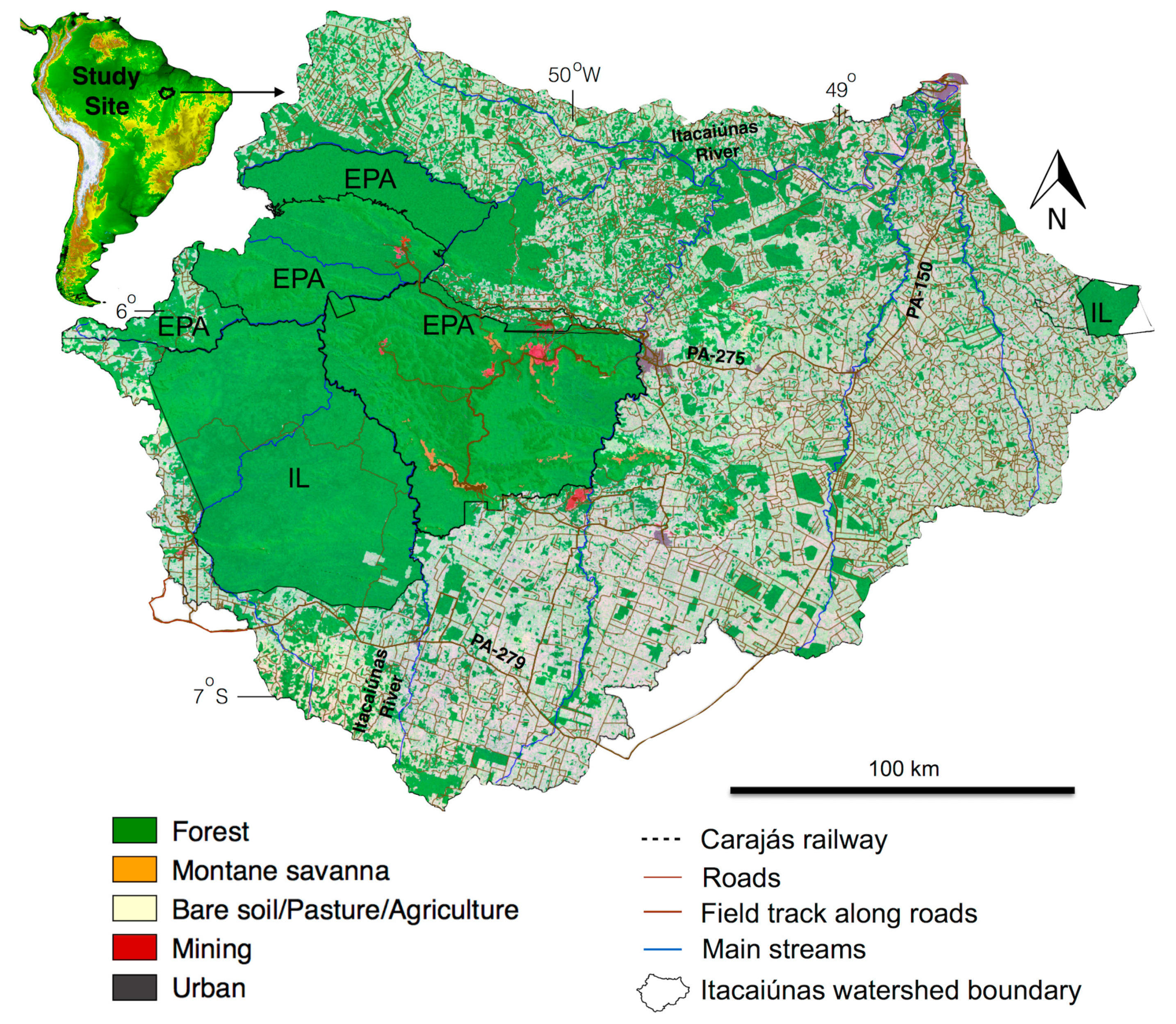
2.1. Study Area

The study area is situated in the IRW, which covers an area of approximately 41,300 km2 in the southeastern area of the Brazilian Amazon region. The IRW has a basin relief marked by the Carajás Ridge, which reaches an altitude of 900 m [23]. In this region, tropical rainforest and montane savanna areas dominated the pristine landscape. During the past two decades, a variety of land uses were established, and pasturelands are predominant in the landscape [20]. By the mid-1970s, the Brazilian government’s strategy for human settlements in the Amazon had changed. Instead of agricultural settlements of small farmers, large development projects such as mining projects, hydroelectric dams and ports for mining exportation were planned and implemented in the Amazon region [24]. One of the main strategies of the Brazilian government to conserve natural forests in the Amazon region was the creation of indigenous lands and protected areas (ILPAs) [25], which stretch across an area of 11,700 km2. This is approximately 25% of the study area (Figure 1).
Mining activity expanded mainly in the context of the Carajás mining projects, which started in the early 1980s. The role of mining activity in the process of clearing forests has been widely considered [18]; however, industrial mining is directly responsible for the conversion of restricted areas covered by forest or mountain savannas in the mining areas [19]. On the other hand, the main driver of LCLU changes in the IRW was associated with the opening of a rudimentary road network associated with settlements and cattle ranching that facilitated inland timber exploitation in the southeastern Amazon region [26,27,28]. From 1973 to 2013, 50% of the tropical rainforest in the IRW (approximately 20,000 km2) was converted to pasturelands [20]. Although cattle ranching remains the dominant form of land use in the Amazon region, large-scale commercial agriculture, such as soybean croplands, have fundamentally changed the landscape in the southeastern Amazon [29,30]. However, in the IRW, large-scale commercial agriculture is still incipient. In the Amazon region, deforestation occurred primarily on larger properties (higher than 500 ha) dominated by large and very large landholders, whose properties were more concentrated in older areas that had better infrastructure, such as roads, and thus, they were connected to markets [31].
Studies on approximately three decades of deforestation in the Amazon demonstrated that LCLU changes have affected the regional hydroclimate [20,32], specifically in the southeastern area of the Amazon, whose geographical position is in climatological (i.e., a tropical zone without a dry season or monsoon) and ecological (i.e., consisting of tropical rainforest and Brazilian savanna) transition zones that have facilitated LCLU changes [20]. At the time of the study, the climate was characterized by monsoons [33], where the average seasonal precipitation was ~1600 mm and 100 mm, distributed in the well-defined wet (November to May) and dry (June to October) seasons, respectively, with mean temperatures ranging from 26 and 28 °C, respectively [34].

2.2. Remote Sensing Dataset and Field Data Collection

In this study, four mosaics containing five images were constructed from 1984, 1994 and 2004 Landsat-5 TM images and 2013 Landsat-8 OLI images. One mosaic of the 2017 Sentinel 2A satellite was composed of twelve images. The images were acquired during the dry season (from May to September) due to minimal cloud coverage (less than 10%). Table S1 provides general information about satellite images used in this study that were downloaded from the United States Geological Survey Earth-Explorer website (http://earthexplorer.usgs.gov). All the images were acquired in the Level 1 Terrain (L1T) format and were orthorectified onto the Universal Transverse Mercator (UTM) cartographic projection, in the WGS84 datum [35]. Fieldwork was carried out between April-May 2014 and August-September 2017 to recognize the LCLU classes using panoramic digital photographs and ground control points (GCPs), which were acquired using a differential global position system with a decimeter-level accuracy for reliable real-time positioning. Along approximately 2400 km of roads in the study site, 2200 GCPs were collected to validate the 2013 Landsat-8 OLI mosaic classification (Figure 1). Training and validation samples were defined per class based on the GCPs (Figure 2). These data were complemented by Google Earth Pro online high-resolution imagery. Despite the up to 30 year difference between the images and field data acquisition, all georeferenced field descriptions and photographs obtained in the field in 2014 and 2017 matched the previous LCLU classes observed in the 1984, 1994 and 2004 Landsat 5 mosaics.
During the processes of visual image analysis and fieldwork data collection, patterns and patches were identified in the landscape using color composite mosaic images. Hence, three land-cover (i.e., forests, montane savannas and water bodies) and three land-use classes (i.e., pasturelands, mining and urban areas) were identified based on Di Gregorio [36], Ellis [37], and Junk [38]. A brief description of each class identified in this study is presented in Figure 2.

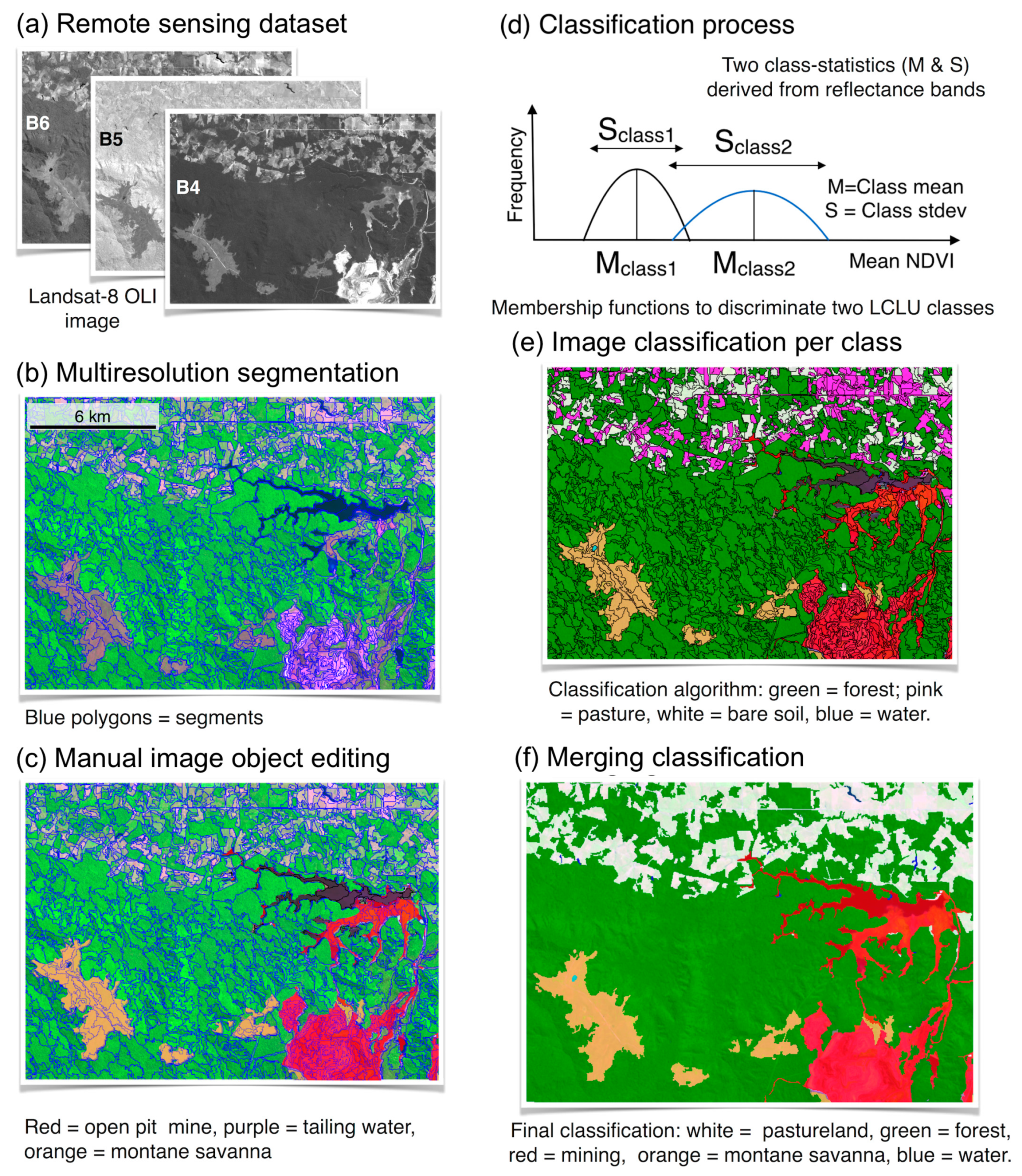
2.3. Digital Image Processing

Each digital number (DN) of 1984, 1994, and 2004 Landsat-5, 2013 Landsat-8 and 2017 Sentinel-2A mosaics were converted to ground reflectance (GR). Conversions from DN to GR were carried out in the Atmospheric Correction (ATCOR) module of the software PCI Geomatica 2016 [39]. For each Landsat and Sentinel mosaic date, we derived the normalized difference vegetation index (NDVI) to identify vegetated areas with exposed soils [40]. We also used the Landsat-8 6/4 band ratio and the Landsat-5 5/3 band ratio, which represent the ratio between the long and short wavelengths, to identify iron ore deposits [41]. NDVI and band ratios were used only during the classification process after image mosaic segmentation. Subsequently, we generated mosaics of Landsat and Sentinel images that were 30 m and 10 m in pixel size respectively, to quantify human-driven changes throughout the IRW.

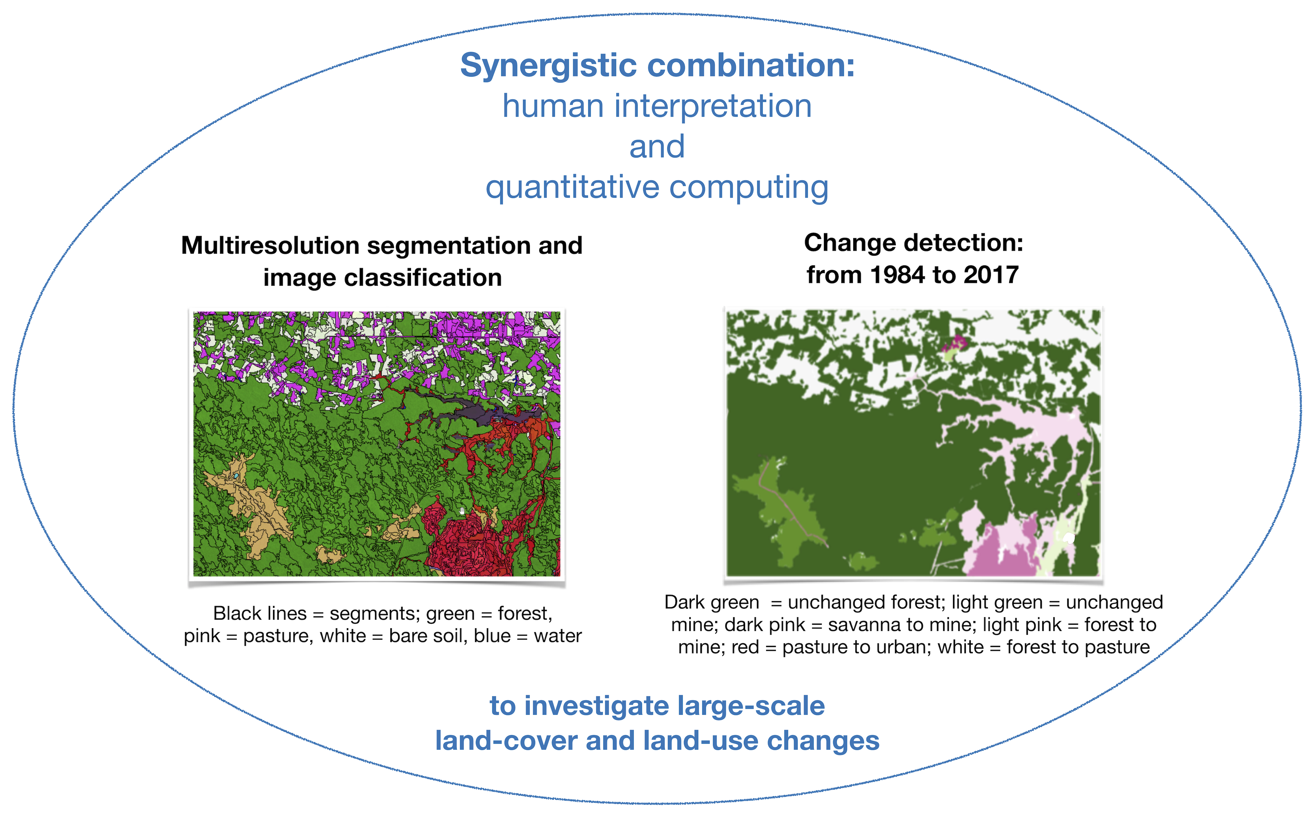
2.4. Geographic Object-Based Image Analysis (GEOBIA)

2.4.1. Segmentation

The segmentation process includes three user-defined parameters: (i) the spectral parameter wsp, trading spectral homogeneity versus object shape, is included in order to obtain spectrally homogenous objects; (ii) the compactness parameter wcp, trading compactness versus smoothness, adjusts the object shape between compact objects and smooth boundaries, and (iii) the scale parameter hsc, which corresponds to the threshold of heterogeneity, controlling the object size has been selected in order that the minimum object size match to the Minimum Mapping Unit (MMU), i.e., the smallest size area entity to be mapped as a discrete area [42].
A multiresolution segmentation algorithm was conducted for the band 2 (B2), B3, B4, B5, B6, B7 and B8 GR reflectance bands of the Landsat-8 OLI images using weights of 5, 15, 15, 10, 15, 15 and 15, respectively. The segmentation procedure was also applied to band 2 (B2), B3, B4, B5, B7, and B5/B3 GR bands of the Landsat-5 TM images using weights of 15, 15, 10, 15, 15 and 5, respectively. The same segmentation process was applied to band 2 (B02), B03, B04 and B08 GR bands of the Sentinel-2A mosaic using weight of 1 to all bands. Different weights were chosen to Landsat bands from a trial and error (heuristics) approach to attempt to enhance specific objects that were effectively differentiated in predetermined spectral bands [43]. Since we were unsure of the relationships between the spectrum versus the shape and between the compactness versus the smoothness, the shape parameters (wsp) and compactness (wcp) were both set equal to 0.5 [11].
In relation to the definition of the scale parameter (hsc), several unsupervised and supervised methods exist to define the optimal scale parameter [44,45]. However, for many authors, the selection of appropriate scale parameter settings has been heavily dependent upon trial and error exploration, which is iterative and time-consuming [46,47,48], due to the lack of an obvious mathematical relationship between the scale parameter and the success of the segmentation [44]. In this study, hsc was progressively increased and set at 50 in the Landsat-8 OLI and Landsat-5 TM multispectral bands and 10 in the Sentinel-2A. The high hsc allowed more heterogeneity and resulted in larger segments [48] that were more adequate to delineate forest and pastureland areas. Hence, each segment in the Landsat mosaics presented a minimum object size (equal to the minimum mapping unit (MMU) of 25,000 m2 or approximately 28 pixels, while in the Sentinel-2A mosaic presented an MMU of 5000 m2 or 50 pixels. Thus, the variation in the size of the segments in both images should be minimal. It is important to mention that “from-to” change analysis was carried out only after the merging classification process. Thus, the size of the original segments does not have much influence on this change detection approach.

2.4.2. Multiresolution Classification

We used membership functions to define the relationship between feature values and the degree of membership to a class using fuzzy logic. This allowed integrating various features in the description of classes by logical operators. During the automatic classification process, we adopted the membership functions to describe specific properties of the objects. The selection of features was assisted by an analysis of separability of the comparable classes (Sample Editor, Image Object Information and Feature View Tools of eCognition Developer 9). Each class was classified separately in the domain of image object level, using the class filter “unclassified”. The classification algorithm was used to delimitate the LCLU classes from a combined manual interpretation and automatic classification synergy from GEOBIA. We observed spectral similarities among the mining, bare soil, and urban classes. Furthermore, since the montane savanna class and the mining and urban areas were represented by a small number of segments, we decided to manually edit the thematic vector objects (mining, urban and montane savanna classes). In essence, this technique combines the advantages of semiautomated fine-level object generation and classification with visual human interpretation [49]. Then, a set of rules was established to automatically classify objects associated with black water bodies, whitewater bodies, bare soil, pasture/croplands, and forest. Posteriorly, black-white water bodies and bare soil-pasture/croplands were grouped through merge region algorithm in two large classes: water bodies and pasturelands. Each class was classified from a simple membership function (e.g., Gaussian—∩, larger than—∫, full range—п), which played a role of thresholds in different spectral bands. Table 1 summarizes the main steps used during the GEOBIA analysis referenced as process tree, the different child process carried out associated to the recognition of different classes, the algorithm used during the multi-resolution segmentation, and the membership function with their intervals.
The selection of features was supported by a separability analysis of the comparable classes. Each class was classified separately on an image-object level, using the class filter “unclassified”, according to the following order: (1) mining, urban and montane savanna classes (manual editing), (2) blackwater bodies, (3) white-water bodies, (4) bare soil, (5) pasture/croplands, and (6) forests (automated classification). Subsequently, black- and white-water bodies and bare soil and pasture/croplands were grouped using an algorithm to merge the regions into two large classes: water bodies and pasturelands, respectively. An overview of the steps of the GEOBIA is illustrated in Figure 3.

2.4.3. Classification Accuracy Assessment of the LCLU Classes

An object-based accuracy assessment is different from a pixel-based validation due to the sampling unit, i.e., objects vs. pixels [50]. However, a generally accepted approach is that classified polygons can be validated by GCPs [51]. To perform the classification accuracy assessment, we used 1060 and 2100 GCPs over 2013 Landsat-8 OLI and 2017 Sentinel-2A mosaics, respectively. As older GCPs and thematic maps were unavailable through 2004, 1994 and 1984 Landsat-5 TM mosaics, 512 validation points were randomly stratified per class in each mosaic using PCI Geomatica 2016 software [39]. The number of training and validation points per class used in each multitemporal image is presented in Figure 2. Hence, an accuracy assessment of the multitemporal Landsat image classification was conducted using nonnormalized and normalized confusion matrices [52]. The producer and user accuracies [53], kappa per class, kappa index of agreement and overall accuracy [51] as well as the quantity disagreement (QD) and allocation disagreement (AD) indexes [54] were calculated for each multitemporal mosaic.

2.4.4. Object-Based Change Detection Analysis

The object-based change detection analysis was performed on the 1984, 1994, 2004 Landsat-5 TM, 2013 Landsat-8 OLI and 2017 Sentinel-2A mosaics. The change detection analysis revealed and quantified either the expansion-contraction or lack of change (no change) of specific classes relative to one another to understand their spatiotemporal dynamics. More specifically, a detailed LCLU “from-to” change detection approach [15] was used to recognize the trajectories of the LCLU classes based on an object-based change detection analysis from 1984–1994, 1994–2004, 2004–2013, 2013–2017 and 1984–2017.
We identified five unchanged classes (forests, montane savannas, pasturelands, and urban and mining areas) and the six main possible change trajectories related to the “from-to” conversions of forests-pastureland, forests-mining areas, forests-urban areas, montane savanna-mining areas, pastureland-forests, and pastureland-urban area. To apply the object-based change detection analysis, we used a hierarchical biannual image object approach.

3. Results

3.1. Overall Classification and Accuracy Assessment of Multitemporal LCLU Maps

A multiresolution classification based on the synergistic combination of manual interpretation and automatic classification with a GEOBIA approach effectively classified the Landsat and Sentinel-2A images into six LCLU classes. Figure 4 shows the LCLU classes distributed throughout the study site during the years 1984, 1994, 2004, 2013 and 2017, with the largest proportion of primary forests occurring in 1984 and its progressive conversion to pastureland occurring by 2017. The overall accuracies of all the classified mosaics are higher than 94%, while the kappa indexes are higher than 0.91, and the AD and QD are lower than 3.5 and 2.0, respectively (Tables S2 and S3). In general, the kappa index per class is higher than 0.8, except for the mining class in 1984 (Figure 5a). Therefore, the overall disagreement is very low. On average, the AD is higher (1.4%) than the QD (0.9%), which is higher only for forest areas in 2004 and 2013, mountain savanna areas in 1994, mining areas in 1984 and 1994, and water each year (Figure 5b). User and producer’s accuracy is higher than 80%, except for the mining class in 1984 (Figure 5c,d).

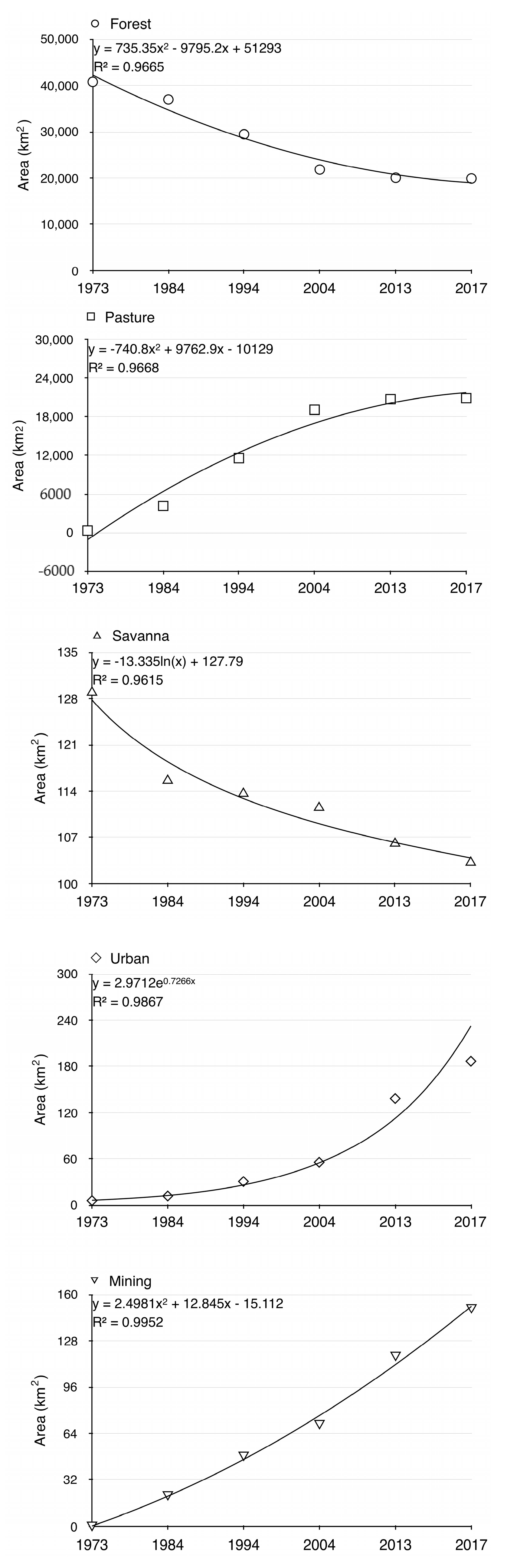
3.2. Analysis of Multitemporal LCLU Changes

The classification results showed that forests occupied most of the study site in 1984 but decreased rapidly in 1994 and 2004. In contrast, pasturelands increased rapidly during the same period and occupied the largest extent of the IRW in 2017. From 1984 to 2017, forest areas were progressively restricted to within ILPAs, while pasturelands were expanded into other areas of the watershed. We can confirm that only a small area of forests was used for pasturelands in 1984 (4.154 km2, which corresponds to 10% of the total studied watershed). However, pasturelands occupied approximately 28%, 46%, 50.2% and 50.6% of the entire watershed in 1994, 2004, 2013 and 2017, respectively. Pasturelands currently correspond to approximately 20,900 km2. Overall, 20,870 km2 of forests have been cleared, mostly due to the expansion of pasturelands. The evolution of the total area of each LCLU class during the studied period is presented in Figure 6. In general, in the ILPAs, the land cover remained almost untouchable in comparison to non-protected areas.
The montane savannas were less affected by land-use dynamics and occupied an area of almost ~116 km2 in 1984. This area was reduced to 103 km2 in 2017, corresponding to a decrease of 11%. Mining activity expanded mainly in the context of the Carajás mining projects, which started in the early 1980s [55]. We observed a simultaneous increase in urban area from 117 km2 in 1984 to 187 km2 in 2017, with more accelerated urban expansion in the past decade.

3.3. LCLU “from-to” Change Detection Analysis

The analysis of the LCLU datasets described above provides an overall dynamic view of the LCLU changes. However, this analysis did not reveal the change trajectories from one LCLU class to another class type. The LCLU areas and the detailed percentages of their unchanged and “from-to” variations among different LCLU classes can be observed in Table 2.
The LCLU change detection analysis between 1984 and 1994 indicates that unchanged forest was the largest class with almost 28,178 km2 (70% of the study area). Approximately 7925 km2 of forest in 1984 was converted to pasturelands in 1994, while 26 km2 and 7 km2 of forests were converted to mining and urban areas, respectively. Unchanged pastureland encompassed ~3100 km2, and secondary forests increased by 652 km2. Approximately 4 km2 of montane savanna was converted to mining areas (Table 2). In the subsequent decade, between 1994 and 2004, the unchanged forest class represented approximately 20,463 km2, while unchanged pastureland covered 10,400 km2. The conversions from forest to pastureland and from forest to mining areas in this period were similar to those observed in the preceding evaluation period. However, the changes from montane savanna to mining areas were 5.6 km2, which is significantly larger than that during the period 1984–1994. Approximately 723 km2 of pasturelands were converted to forests. The change detection analysis between 2004 and 2013 and 2013 to 2017 was marked by an accentuated decrease in LCLU changes, with unchanged forests and unchanged pasturelands occupying areas of approximately 18,000 km2. The conversion from forest to pastureland was halved in that time, while forest recovery from pasturelands reached its maximum intensity (1400 km2). This finding indicates a clear tendency of stabilization of the LCLU changes in the watershed in the last decade. Throughout the period of change detection (1984–2017), we observed that 47% of the area was still covered by forests and patches of forests. Almost 42% of the LCLU changes were associated with the conversion from forests to pasturelands (~17,400 km2), while 3.505 km2 remained as unchanged pasturelands. Figure 7 illustrates the unchanged LCLU classes and the “from-to” change detection classes based on a bi-temporal mosaic image analysis.
The “from-to” change detection analysis revealed that forests were converted mainly into pasturelands, with annual rates greater than 720 km2 per year from 1984 to 1994 and from 1994 to 2004. However, from 2004 to 2013 and from 2013 to 2017, the conversion rate decreased to 300 and 326 km2 per year, respectively, as well as an increase in the regrowth of forest-like vegetation (secondary forest) in the pasturelands occurred (Figure 8a). Furthermore, a clearly increasing trend in the conversion of forests to mining areas and savanna to mine areas was observed (Figure 8b). The conversion of pastureland into forest-like vegetation was only detectable due to the “from-to” changes detection approach.

4. Discussion

4.1. Issues of Accuracy for Multitemporal LCLU Classes

The accuracies yielded for the four decadal image classifications were highly satisfactory (Figure 5, Tables S2 and S3), but some considerations regarding the number and spatial distribution of the validation points are important. The collection of validation points in the field for the more recent images was constrained by accessibility, so that their spatial distributions may be not ideal statistically (e.g., randomly distributed). Consequently, it is likely that some points will carry the effect of spatial autocorrelation, resulting in the measured agreement being higher [56]. However, the accuracy was similar to that of the other three scenarios providing some confidence that this was not significant since their sampling schema was different based on stratified map units and visual recognition. Moreover, this result suggests that the validation strategy was consistent throughout the series of the LULC maps.
Another consideration is that the overall accuracy and kappa index [57] were intended to measure the degree of agreement with the validation points, with no information about the nature of disagreements. For this purpose, AD and QD provided measures of discordance due to the imperfect spatial allocation of class polygons and due to the incorrect extent of classes, respectively [54]. Allocation disagreement is important to change detection as spatial mismatches during map comparisons may result with the detection of false transitions. Quantity disagreement, on the other hand, is important when the aim is to compute areal differences in classes among maps. In this study, AD was approximately 1.5 times greater than the quantity most of the time, indicating that the area of the classes tended to be more accurate for this purpose. However, the change detection between different years tended to be less reliable than the computed areas; however, as both measures were never low, none of the results were expected to be significantly affected.
Nevertheless, additional information about specific classes can be obtained from the confusion matrices (Tables S2 and S3). Producer accuracy and omission error, for example, show how well the validation points were classified in the maps of LCLU [52,58]. The producer accuracies were relatively close in value and uniform for all classes in all mosaics, in general above 90%, and thus, the omission errors were correspondingly low. The user accuracy and commission error show how “pure” a class tends to be and the proportion of different classes that have been assigned to it, respectively [58]. These measures presented higher variation between classes and between years, meaning that sometimes certain classes included major proportions of other classes, which was more noticeable for classes with small occurrences. Mining, for example, presented the lowest user accuracy in three of the four decadal images (1984, 1994 and 2013), with corresponding higher commission errors. Therefore, changes related to small classes probably were overestimated.

4.2. LCLU Assessment Using Time Series Satellite Images and GEOBIA

The high classification accuracies of the satellite images were due to a combination of the ability of visual human interpretation to recognize and define specific classes (e.g., mining and urban areas) with those of an automated fine-level object classification (e.g., forest, bare soil, pastureland-cropland and water bodies).

4.3. LCLU “from-to” Change Detection Approach

The object-based change detection approach for unchanged and “from-to” variations in the LCLU showed that approximately 50% of the forests remained, while the other 50% was converted into pasturelands. Figure 9a shows the strong negative correlation between forests versus pasturelands throughout the past four decades, which suggests that the incremental growth in pastureland is directly related to deforestation processes. Throughout the whole Amazon region, the Amazon arc of deforestation has had the highest rates of deforestation [59] since the opening of roads in the beginning of the 1970s, which allowed the establishment of new rural settlements and the expansion of pasturelands [26,27]. In addition, deforestation occurred preferentially on larger properties with >500 ha dominated by large and very large landholders, whose properties were more concentrated in older areas that had better infrastructure, such as roads, and thus were connected to markets [31]. The scars of the initial forest exploration efforts can be observed in the 1984 classified mosaic images; those scars expanded gradually along the roads over the subsequent decades (Figure 4). A clear spatial relationship between this expansion and the location of major roads, such as PA-275, PA-279 and PA-150, existed (Figure 1). Hence, one of the greatest environmental impacts associated with the conversion of forests to pasturelands over the past 30 years was related to pronounced climatic and hydrological changes, which were responsible for decreases in relative humidity and increases in air temperatures and water river discharges [20].
Mining activity typically contributes substantially to deforestation [60]. However, the findings demonstrate that the mining area represents less than 0.3% of the deforested area in the context of the IRW. Hence, we can conclude that the role of mining activities in deforestation processes was slight. Moreover, collaboration between the governmental agencies responsible for environmental management and mining companies was recognized as essential to ensuring forest preservation in protected areas [61]. At the same time, the expansion of mining areas was only significant in the montane savannas, 20% of which were converted into mining areas by 2017. A high negative correlation between montane savanna versus mining and montane savanna versus forest areas has been found since the expansion of mining areas has been focused to the savannas and forests (Figure 9b,c). This correlation was not inclusive because the largest expansion of the mining areas originated from forests (Table 2). To explain the low conversion rate of pristine land-cover types into mining areas, we noted that mining activities are subjected to strict environmental rules and are strongly controlled by government agencies. In addition, a large part of this conversion occurred within protected areas, which reinforces the need for constraints on mining exploration. These results represent the first estimates of land-cover conversion to mining areas within the CMP, largest mining province of the Brazilian Amazon region. Previous studies have evaluated only the impact of gold mining in the Madre de Dios region of the Peruvian Amazon [16]. In that area, LCLU changes have been recorded by high-spatial-resolution satellite images, and the ecosystem destruction related to gold extraction has been estimated as the loss of approximately 19 km2 of forests per year from 2006 to 2009. This rate of deforestation was much more intense than that observed in the CMP, where the maximum annual deforestation rates reached 4.6 km2 per year over the past five years. Therefore, mining projects were responsible for only a small proportion of direct land-use changes in the study site. In other words, mining activities in the CMP can be considered more sustainable to miners, communities, customers and the environment, when compared with other mining sites in South America [62].
Urban expansion occurred principally within pasturelands, whose area stabilized from 2013 (Figure 6, pasture), while urban area is still increasing (Figure 6, urban; Figure 9d). The increased annual rates of urban growth showed behavior similar to that of mining activity in that both showed a high positive correlation (Figure 9e). The annual rate of mining expansion during the 1980s increased more rapidly than that of urban expansion. We can explain the expansion of mining in the first two decades as a consequence of the development and implementation of the Carajás Mineral Program from 1979 to 1990 [24]. As a result of the development and expansion of the Carajás polymetallic ore mining complex, during the last decade, employment pressure for the large projects has gradually increased, promoting the growth of small villages at the foot of the ridge and inducing a rapid and uncontrolled expansion of urban areas [63].

5. Conclusions

The methodological approach used in this study combined the advantages of visual human interpretation of segmented images to identify and define specific classes (e.g., mining and urban areas) with those of an automated fine-level object classification (e.g., for forest, bare soil, pastureland-cropland and water bodies). Moreover, we observed that forests were converted primarily into pasturelands and that urban areas have been expanded due to the establishment of different human-related activities.
We conclude that the synergistic combination of manual interpretation (the aggregation and discrimination of fine-level objects at a high contrast in association with urban, mining and montane savanna classes) with automatic classification (for coarse-level objects related to forests and pasturelands) is more effective when there is a need to avoid misclassification of objects with similar features. This approach combines the advantages of quality human interpretation with the capacities of quantitative computing. Therefore, this study is useful for not only practitioners working across tropical regions but also those who investigate large-scale LULC changes and those interested in using remote sensing data for conservation tasks.

Supplementary Materials

The following are available online at https://www.mdpi.com/2072-4292/10/11/1683/s1, Tables S1–S3.

Author Contributions

Conceptualization, P.W.M.S.-F.; fieldwork collection, P.W.M.S.-F., R.O.S.J., digital image processing, P.W.M.S.-F., W.R.N.J., D.C.S., GIS analysis, P.W.M.S.-F., W.R.N.J., D.C.S.; formal analysis, P.W.M.S.-F., W.R.N.J., R.O.S.J., funding acquisition, J.O.S.; accuracy assessment, P.W.M.S.F., E.J.W., D.C.S., writing—original draft preparation, P.W.M.S.-F.; review & editing, P.W.M.S.-F., E.J.W., J.O.S.

Funding

This research received no external funding. The authors P.W.M.S.-F.; and D.C.S. was funded by Brazilian Research National Council (CNPq), research grant numbers 306450/2013-5, 302839/2016-0, and 3029382/2018, respectively.

Acknowledgments

The authors would like to thank the United States Geological Survey for providing the Landsat-8 OLI and Landsat-5 TM images. This project was partially conducted in the National Forest of Carajás with the permission of IBAMA (SISBIO 35594-2). The manuscript benefited significantly from the journal’s reviewers.

Conflicts of Interest

The authors declare no conflict of interest.

References

  1. Singh, A. Review article digital change detection techniques using remotely-sensed data. Int. J. Remote Sens. 1989, 10, 989–1003. [Google Scholar] [CrossRef]
  2. Lu, D.; Li, G.; Moran, E.; Hetrick, S. Spatiotemporal analysis of land-use and land-cover change in the brazilian amazon. Int. J. Remote Sens. 2013, 34, 5953–5978. [Google Scholar] [CrossRef] [PubMed]
  3. Blaschke, T.; Hay, G.J.; Kelly, M.; Lang, S.; Hofmann, P.; Addink, E.; Queiroz Feitosa, R.; van der Meer, F.; van der Werff, H.; van Coillie, F.; et al. Geographic object-based image analysis—Towards a new paradigm. ISPRS J. Photogramm. Remote Sens. 2014, 87, 180–191. [Google Scholar] [CrossRef] [PubMed]
  4. Burnett, C.; Blaschke, T. A multi-scale segmentation/object relationship modelling methodology for landscape analysis. Ecol. Model. 2003, 168, 233–249. [Google Scholar] [CrossRef]
  5. Liu, D.; Xia, F. Assessing object-based classification: Advantages and limitations. Remote Sens. Lett. 2010, 1, 187–194. [Google Scholar] [CrossRef]
  6. Platt, R.V.; Rapoza, L. An evaluation of an object-oriented paradigm for land use/land cover classification. Prof. Geogr. 2008, 60, 87–100. [Google Scholar] [CrossRef]
  7. Tompoulidou, M.; Gitas, I.Z.; Polychronaki, A.; Mallinis, G. A GEOBIA framework for the implementation of national and international forest definitions using very high spatial resolution optical satellite data. Geocarto Int. 2016, 31, 342–354. [Google Scholar] [CrossRef]
  8. Garcia-Pedrero, A.; Gonzalo-Martin, C.; Fonseca-Luengo, D.; Lillo-Saavedra, M. A GEOBIA methodology for fragmented agricultural landscapes. Remote Sens. 2015, 7, 767–787. [Google Scholar] [CrossRef]
  9. Blaschke, T. Object based image analysis for remote sensing. ISPRS J. Photogramm. Remote Sens. 2010, 65, 2–16. [Google Scholar] [CrossRef]
  10. Chen, G.; Hay, G.J.; Carvalho, L.M.T.; Wulder, M.A. Object-based change detection. Int. J. Remote Sens. 2012, 33, 4434–4457. [Google Scholar] [CrossRef]
  11. Desclée, B.; Bogaert, P.; Defourny, P. Forest change detection by statistical object-based method. Remote Sens. Environ. 2006, 102, 1–11. [Google Scholar] [CrossRef]
  12. Lyons, M.B.; Phinn, S.R.; Roelfsema, C.M. Long term land cover and seagrass mapping using landsat and object-based image analysis from 1972 to 2010 in the coastal environment of south east queensland, australia. ISPRS J. Photogramm. Remote Sens. 2012, 71, 34–46. [Google Scholar] [CrossRef]
  13. Nascimento, W.R., Jr.; Souza-Filho, P.W.M.; Proisy, C.; Lucas, R.M.; Rosenqvist, A. Mapping changes in the largest continuous amazonian mangrove belt using object-based classification of multisensor satellite imagery. Estuar. Coast. Shelf Sci. 2013, 117, 83–93. [Google Scholar] [CrossRef]
  14. Chen, J.M.; Chen, J.M.; Liao, A.; Cao, X.; Chen, L.; Chen, X.; He, C.; Han, G.; Peng, S.; Lu, M.; et al. Global land cover mapping at 30 m resolution: A pok-based operational approach. ISPRS J. Photogramm. Remote Sens. 2015, 103, 7–27. [Google Scholar] [CrossRef]
  15. Lu, D.; Li, G.; Moran, E. Current situation and needs of change detection techniques. Int. J. Image Data Fusion 2014, 5, 13–38. [Google Scholar] [CrossRef]
  16. Asner, G.P.; Llactayo, W.; Tupayachi, R.; Luna, E.R. Elevated rates of gold mining in the amazon revealed through high-resolution monitoring. Proc. Natl. Acad. Sci. USA 2013, 110, 18454–18459. [Google Scholar] [CrossRef] [PubMed]
  17. Sonter, L.J.; Moran, C.J.; Barrett, D.J.; Soares-Filho, B.S. Processes of land use change in mining regions. J. Clean. Prod. 2014, 84, 494–501. [Google Scholar] [CrossRef] [Green Version]
  18. Sonter, L.J.; Herrera, D.; Barrett, D.J.; Galford, G.L.; Moran, C.J.; Soares-Filho, B.S. Mining drives extensive deforestation in the brazilian amazon. Nat. Commun. 2017, 8, 1013. [Google Scholar] [CrossRef] [PubMed]
  19. Lobo, F.; Souza-Filho, P.; Novo, E.; Carlos, F.; Barbosa, C. Mapping mining areas in the brazilian amazon using msi/sentinel-2 imagery (2017). Remote Sens. 2018, 10, 1178. [Google Scholar] [CrossRef]
  20. Souza-Filho, P.W.M.; de Souza, E.B.; Silva Júnior, R.O.; Nascimento, W.R., Jr.; Versiani de Mendonça, B.R.; Guimarães, J.T.F.; Dall’Agnol, R.; Siqueira, J.O. Four decades of land-cover, land-use and hydroclimatology changes in the itacaiúnas river watershed, southeastern amazon. J. Environ. Manag. 2016, 167, 175–184. [Google Scholar] [CrossRef] [PubMed]
  21. Costa, M.H.; Botta, A.; Cardille, J.A. Effects of large-scale changes in land cover on the discharge of the tocantins river, southeastern amazonia. J. Hydrol. 2003, 283, 206–217. [Google Scholar] [CrossRef]
  22. Silva Júnior, R.O.; de Souza, E.B.; Tavares, A.L.; Mota, J.A.; Ferreira, D.B.S.; Souza-Filho, P.W.M.; da Rocha, E.J.P. Three decades of reference evapotranspiration estimates for a tropical watershed in the eastern amazon. Anais Acad. Bras. Cienc. 2017, 89, 1985–2002. [Google Scholar] [CrossRef] [PubMed]
  23. Piló, L.B.; Auler, A.S.; Martins, F.D. Carajás national forest: Iron ore plateaus and caves in southeastern amazon. In Landscapes and Landforms of Brazil; Vieira, B.C., Salgado, A.A.R., Santos, L.J.C., Eds.; Springer: Berlin, Germany, 2015; pp. 273–283. [Google Scholar]
  24. Diegues, A.C.; Millikan, E.C.B.; Ferraz, I.T.; Hebette, J. Deforestation and Livelihoods in the Brazilian Amazon; NUPAUB: São Paulo, Brazil, 1997; p. 189. [Google Scholar]
  25. Nepstad, D.; Schwartzman, S.; Bamberger, B.; Santilli, M.; Ray, D.; Schlesinger, P.; Lefebvre, P.; Alencar, A.; Prinz, E.; Fiske, G.; et al. Inhibition of amazon deforestation and fire by parks and indigenous lands. Conserv. Boil. 2006, 20, 65–73. [Google Scholar] [CrossRef]
  26. Laurance, W.F.; Goosem, M.; Laurance, S.G.W. Impacts of roads and linear clearings on tropical forests. Trends Ecol. Evol. 2009, 24, 659–669. [Google Scholar] [CrossRef] [PubMed] [Green Version]
  27. Barber, C.P.; Cochrane, M.A.; Souza, C.M., Jr.; Laurance, W.F. Roads, deforestation, and the mitigating effect of protected areas in the amazon. Boil. Conserv. 2014, 177, 203–209. [Google Scholar] [CrossRef]
  28. Uhl, C.; Buschbacher, R. A disturbing synergism between cattle ranch burning practices and selective tree harvesting in the eastern amazon. Biotropica 1985, 17, 265–268. [Google Scholar] [CrossRef]
  29. Morton, D.C.; DeFries, R.S.; Shimabukuro, Y.E.; Anderson, L.O.; Arai, E.; del Bon Espirito-Santo, F.; Freitas, R.; Morisette, J. Cropland expansion changes deforestation dynamics in the southern brazilian amazon. Proc. Natl. Acad. Sci. USA 2006, 103, 14637–14641. [Google Scholar] [CrossRef] [PubMed]
  30. Martinelli, L.A.; Naylor, R.; Vitousek, P.M.; Moutinho, P. Agriculture in brazil: Impacts, costs, and opportunities for a sustainable future. Curr. Opin. Environ. Sustain. 2010, 2, 431–438. [Google Scholar] [CrossRef]
  31. Godar, J.; Gardner, T.A.; Tizado, E.J.; Pacheco, P. Actor-specific contributions to the deforestation slowdown in the brazilian amazon. Proc. Natl. Acad. Sci. USA 2014, 111, 15591–15596. [Google Scholar] [CrossRef] [PubMed]
  32. Khanna, J.; Medvigy, D.; Fueglistaler, S.; Walko, R. Regional dry-season climate changes due to three decades of amazonian deforestation. Nat. Clim. Chang. 2017, 7, 200–204. [Google Scholar] [CrossRef]
  33. Alvares, C.A.; Stape, J.L.; Sentelhas, P.C.; Gonçalves, J.L.M.; Sparovek, G. Koppen’s climate classification map for brazil. Meteorol. Z. 2013, 22, 711–728. [Google Scholar] [CrossRef]
  34. Moraes, B.C.; Costa, J.M.N.; Costa, A.C.L.; Costa, M.H. Variação espacial e temporal da precipitação no estado do pará. Acta Amazon. 2005, 35, 207–214. [Google Scholar] [CrossRef]
  35. Irons, J.R.; Dwyer, J.L.; Barsi, J.A. The next landsat satellite: The landsat data continuity mission. Remote Sens. Environ. 2012, 122, 11–21. [Google Scholar] [CrossRef]
  36. Di Gregorio, A. Land Cover Classification System: Classification Concepts and User Manual; UNEP-FAO: Roma, Italy, 2005. [Google Scholar]
  37. Ellis, E.C.; Ramankutty, N. Putting people in the map: Anthropogenic biomes of the world. Front. Ecol. Environ. 2007, 6, 439–447. [Google Scholar] [CrossRef]
  38. Junk, W.J.; Piedade, M.T.F.; Schöngart, J.; Cohn-Haft, M.; Adeney, J.; Wittmann, F. A classification of major naturally-occurring amazonian lowland wetlands. Wetlands 2011, 31, 623–640. [Google Scholar] [CrossRef]
  39. PCI Geomatica. Geomatica ii: Course Guide. Version 0.2; PCI Geomatics: Markham, ON, Canada, 2015; p. 169. [Google Scholar]
  40. Tarpley, J.D.; Schneider, S.R.; Money, R.L. Global vegetation indices from the noaa-7 meteorological satellite. J. Clim. Appl. Meteorol. 1984, 23, 491–494. [Google Scholar] [CrossRef]
  41. Crippen, R.E. Selection of landsat tm band and band-ratio combinations to maximize lithologic information in color composite displays. In Proceedings of the 7th Thematic Conference on Remote Sensing for Exploration Geology II, Calgary, AB, Canada, 2–6 October 1989; pp. 912–921. [Google Scholar]
  42. Saura, S. Effects of minimum mapping unit on land cover data spatial configuration and composition. Int. J. Remote Sens. 2002, 23, 4853–4880. [Google Scholar] [CrossRef]
  43. Baatz, M.; Schape, A. Multiresolution segmentation: An optimization approach for high quality multi-scale image segmentation. In Angewandte Geographische Informationsverarbeitung; Strbl, J., Blaschke, T., Eds.; Wichmann: Heidelberg, Germany, 2000; pp. 12–23. [Google Scholar]
  44. Zhang, X.; Tong, H.; Chen, X. Multi-scale segmentation algorithm parameters optimization based on evolutionary computation. In Proceedings of the 6th International Symposium Computational Intelligence and Intelligent Systems: Isica 2012, Wuhan, China, 27–28 October 2012; Li, Z., Li, X., Liu, Y., Cai, Z., Eds.; Springer: Berlin/Heidelberg, Germany, 2012; pp. 347–358. [Google Scholar]
  45. Drăguţ, L.; Tiede, D.; Levick, S.R. Esp: A tool to estimate scale parameter for multiresolution image segmentation of remotely sensed data. Int. J. Geogr. Inf. Sci. 2010, 24, 859–871. [Google Scholar] [CrossRef]
  46. Kavzoglu, T.; Erdemir, M.Y.; Tonbul, H. A region-based multi-scale approach for object-based image analysis. Int. Arch. Photogramm. Remote Sens. Spat. Inf. Sci. 2016, XLI-B7, 241–247. [Google Scholar] [CrossRef]
  47. Lowe, S.H.; Guo, X. Detecting an optimal scale parameter in object-oriented classification. IEEE J. Sel. Top. Appl. Earth Obs. Remote Sens. 2011, 4, 890–895. [Google Scholar] [CrossRef]
  48. Mesner, N.; Ostir, K. Investigating the impact of spatial and spectral resolution of satellite images on segmentation quality. APPRES 2014, 8, 1–14. [Google Scholar] [CrossRef]
  49. Benz, U.C.; Hofmann, P.; Willhauck, G.; Lingenfelder, I.; Heynen, M. Multi-resolution, object-oriented fuzzy analysis of remote sensing data for gis-ready information. ISPRS J. Photogramm. Remote Sens. 2004, 58, 239–258. [Google Scholar] [CrossRef]
  50. Radoux, J.; Bogaert, P.; Fasbender, D.; Defourny, P. Thematic accuracy assessment of geographic object-based image classification. Int. J. Geogr. Inf. Sci. 2011, 25, 895–911. [Google Scholar] [CrossRef]
  51. Congalton, R.G.; Green, K. Assessing the Accuracy of Remotely Sensed Data: Principles and Practices, 2nd ed.; CRC Press Taylor & Francis Group: Boca Raton, FL, USA, 2009; p. 183. [Google Scholar]
  52. Congalton, R.G. A review of assessing the accuracy of classifications of remotely sensed data. Remote Sens. Environ. 1991, 37, 35–46. [Google Scholar] [CrossRef]
  53. Story, M.; Congalton, R. Accuracy assessment—A user’s perspective. Photogramm. Eng. Remote Sens. 1986, 52, 397–399. [Google Scholar]
  54. Pontius, R.G.; Millones, M. Death to kappa: Birth of quantity disagreement and allocation disagreement for accuracy assessment. Int. J. Remote Sens. 2011, 32, 4407–4429. [Google Scholar] [CrossRef]
  55. Sa, P.; Marques, I. The carajas iron ore project: The strategy of a third world state- owned enterprise in a depressed market. Resour. Policy 1985, 11, 245–256. [Google Scholar]
  56. Guiot, J.; de Vernal, A. Is spatial autocorrelation introducing biases in the apparent accuracy of paleoclimatic reconstructions? Quat. Sci. Rev. 2011, 30, 1965–1972. [Google Scholar] [CrossRef]
  57. Cohen, J. A coefficient of agreement for nominal scales. Educ. Psychol. Meas. 1960, XX, 37–46. [Google Scholar] [CrossRef]
  58. Foody, G.M. Status of land cover classification accuracy assessment. Remote Sens. Environ. 2002, 80, 185–201. [Google Scholar] [CrossRef]
  59. Fearnside, P.M. Deforestation in brazilian amazonia: History, rates, and consequences deforestación en la amazonía brasileña: Historia, tasas y consecuencias. Conserv. Boil. 2005, 19, 680–688. [Google Scholar] [CrossRef]
  60. Ferreira, J.; Aragão, L.E.O.C.; Barlow, J.; Barreto, P.; Berenguer, E.; Bustamante, M.; Gardner, T.A.; Lees, A.C.; Lima, A.; Louzada, J.; et al. Brazil’s environmental leadership at risk: Mining and dams threaten protected areas. Science 2014, 346, 706–707. [Google Scholar] [CrossRef] [PubMed]
  61. Martins, F.D.; Mendonça, M.V. Floresta nacional de carajás: Compatibilizando a mineração com a preservação. In A Diversidade Cabe Na Unidade?: Áreas Protegidas Do Brasil; Bensusan, N., Prates, A.P., Eds.; IEB: Brasília, Brazil, 2014; pp. 580–591. [Google Scholar]
  62. Souza-Filho, P.W.M.; Gianninia, T.C.; Jaffé, R.; Furtini Neto, A.E.; Gastauer, M.; Oliveiraa, G.; Mota, J.A.; Guimarães, J.T.F.; De Souza, E.B.; Imperatriz-Fonseca, V.L.; et al. Understanding sustainable development in mining based on science oriented approach: A study case in the carajás mineral province, amazon region, brazil. Resour. Policy 2018. in review. [Google Scholar]
  63. Roberts, J.T. Squatters and urban growth in amazonia. Geogr. Rev. 1992, 82, 441–457. [Google Scholar] [CrossRef]
Figure 1. Map of the study area on the 2013 LCLU map generated from an interpretation of Landsat-8 OLI mosaic images. IL = indigenous lands; EPA = environmental protected areas.
Remotesensing 10 01683 g001
Figure 2. Description of land-cover and land-use classification system in this study.
Remotesensing 10 01683 g002
Figure 3. Empirical GEOBIA workflow that illustrates the principles of the segmentation procedure: (a) remote sensing data set analysis, (b) multiresolution segmentation, (c) manual image object editing, (d) classification process based on segmentation, (e) image classification per class, and (f) merging and quantifying the classifications, which incorporates GIS concepts.
Remotesensing 10 01683 g003
Figure 4. (Left) Classified Landsat images showing temporal and spatial variations in LCLU in the IRW for the years 1984 (a), 1994 (b), 2004 (c), 2013 (d), and 2017 (e) (modified from [20]). (Center) A specific site in the IRW illustrated from color composite Landsat images. (Right) Maps generated from GEOBIA.
Remotesensing 10 01683 g004
Figure 5. Kappa index (a), allocation and quantity disagreements (b), user (c) and producer’s (d) accuracy per class for 1984, 1994, 2004, 2013 and 2017mosaic images in the IRW.
Remotesensing 10 01683 g005
Figure 6. Land-cover and land-use area changes in the IRW from 1984 to 2017.
Remotesensing 10 01683 g006
Figure 7. (Left) Distribution of LCLU changes from the object-based approach during the periods 1984–1994 (a) 1994–2004 (b) 2004–2013 (c) 2013-2017 (d) and 1984–2013 (e) in the IRW. (Right) Detailed maps illustrating LCLU changes using the “from-to” change detection approach.
Remotesensing 10 01683 g007
Figure 8. Annual conversion rates of major land-cover to land-use classes. (a) Forests to pasture, pasture to forest and forest to mine. (b) Forests to mine, forests to urban and montane savannas to mine.
Remotesensing 10 01683 g008
Figure 9. Correlations between the LCLU class areas from 1984 to 2013 based on the dataset in Table 2: (a) forests and pasturelands; (b) montane savannas and mining areas; (c) mining and urban areas; (d) pastureland and urban; and (e) urban and mining.
Remotesensing 10 01683 g009
Table 1. The process tree, child processes, algorithms, and membership functions used in the LCLU classification following the GEOBIA approach.
Process TreeChild ProcessesAlgorithmMembership Functions with Their Intervals
OLI BandsTM BandsSentinel 2A
1. Segmentation Multiresolution segmentationhsc = 50
wsp = 0.5
wcp = 0.5
hsc = 50
wsp = 0.5
wcp = 0.5
hsc = 10
wsp = 0.5
wcp = 0.5
2. Classification(2.1) Classify black-water bodiesClassification, filter unclassified Remotesensing 10 01683 i001B5: 3.78–15.7 Remotesensing 10 01683 i003B2: 4.2–6.9 Remotesensing 10 01683 i004NDVI: −0.9–0.5
Remotesensing 10 01683 i001B6: 0.6–12.3 Remotesensing 10 01683 i005B3: 4.6–7.4
Remotesensing 10 01683 i001B7: 0.5–10.4 Remotesensing 10 01683 i003B4: 4.9–8.9
Remotesensing 10 01683 i003B5: 0.78–3.6
(2.2) Classify white-water bodiesClassification, filter unclassified Remotesensing 10 01683 i001B1: 4.8–10.6 Remotesensing 10 01683 i001B2: 5.1–11.3 Remotesensing 10 01683 i004NDVI: −0.9–0.5
Remotesensing 10 01683 i001B4: 0.9–13.1 Remotesensing 10 01683 i001B3: 5.6–12.6
Remotesensing 10 01683 i001B5: 4.1–22.2 Remotesensing 10 01683 i001B4: 4.2–24.4
Remotesensing 10 01683 i001B5: 0.8–14.9
(2.3) Classify bare soilClassification, filter unclassified Remotesensing 10 01683 i001B3: 1.8–4.1 Remotesensing 10 01683 i001B3: 6.3–25.1
Remotesensing 10 01683 i001B8: 1.5–2.9 Remotesensing 10 01683 i004NDVI: 8.4–64.4
(2.4) Classify Pasture/agricultureClassification, filter unclassified Remotesensing 10 01683 i002B5: 22.2–45.3 Remotesensing 10 01683 i002Bg *: 8.4–14.3 Remotesensing 10 01683 i004B03: 5.4–11
Remotesensing 10 01683 i002B8: 5.7–9.2 Remotesensing 10 01683 i002B2: 4.6–10.4 Remotesensing 10 01683 i004B04: 3.5–7
Remotesensing 10 01683 i002B4: 27.6–48.1 Remotesensing 10 01683 i006not forest:
Remotesensing 10 01683 i002B5: 11.7–32.9
(2.5) Classify forestClassification, filter unclassified Remotesensing 10 01683 i001MD *: 0.9–1.5 Remotesensing 10 01683 i001MD *: 24–39 Remotesensing 10 01683 i004MD *: 0.1–0.4
Remotesensing 10 01683 i004B04: 0–6
3. Group(3.1) Group black and white-water bodiesMerge region
(3.2) Group soil, pasture, agricultureMerge region
* Bg = Brightness, MD = Maxima Difference, B = spectral band, hsc = parameter scale, wsp= shape parameters, wcp = compactness parameters.
Table 2. Summary of LCLU class change trajectories from the object-based approach between 1984–1994, 1994–2004, 2004–2013, 2013–2017 and 1984–2017.
LCLU Change Class1984–19941994–20042004–20132013–20171984–2017
Area (km2)%Area (km2)%Area (km2)%Area (km2)%Area (km2)%
Forest—Mine26.330.0724.890.0636.440.0922.940.06111.380.27
Forest—Pasture7924.7619.817956.4520.023006.227.541632.033.9717,397.9342.23
Forest—Urban7.180.024.220.018.960.021.970.0091.490.22
Pasture—Forest652.101.63722.591.821387.833.481432.813.48555.061.35
Pasture—Urban12.260.030.000.0075.150.1955.990.1482.180.20
Savanna—Mine3.880.015.600.014.860.0111.720.0322.660.06
Unchanged Forest28,178.4770.4420,462.8951.5018,070.9145.3018,392.9344.7319,319.2446.89
Unchanged Mining13.590.0334.010.0954.890.14117.190.2820.860.05
Unchanged Savanna102.260.2699.320.2594.240.2486.040.2182.440.20
Unchanged Pasture3073.037.6810,398.9426.1717,102.4842.8719,227.5746.763502.218.50
Unchanged Urban11.310.0327.420.0751.000.13138.210.3413.540.03

