Hyperspectral Classification via Superpixel Kernel Learning-Based Low Rank Representation

Abstract

High dimensional image classification is a fundamental technique for information retrieval from hyperspectral remote sensing data. However, data quality is readily affected by the atmosphere and noise in the imaging process, which makes it difficult to achieve good classification performance. In this paper, multiple kernel learning-based low rank representation at superpixel level (Sp_MKL_LRR) is proposed to improve the classification accuracy for hyperspectral images. Superpixels are generated first from the hyperspectral image to reduce noise effect and form homogeneous regions. An optimal superpixel kernel parameter is then selected by the kernel matrix using a multiple kernel learning framework. Finally, a kernel low rank representation is applied to classify the hyperspectral image. The proposed method offers two advantages. (1) The global correlation constraint is exploited by the low rank representation, while the local neighborhood information is extracted as the superpixel kernel adaptively learns the high-dimensional manifold features of the samples in each class; (2) It can meet the challenges of multiscale feature learning and adaptive parameter determination in the conventional kernel methods. Experimental results on several hyperspectral image datasets demonstrate that the proposed method outperforms several state-of-the-art classifiers tested in terms of overall accuracy, average accuracy, and kappa statistic.

1. Introduction

The hyperspectral image (HSI) reflects information on hundreds of adjacent narrow spectral bands collected by the airborne or space-borne hyperspectral imagers. Abundant spectral information for HSI makes it suitable for many important applications, such as mineral exploration [1], agricultural production [2], and military target detection [3,4]. Thus, HSI classification is a hotspot in the field of remote sensing image processing [5,6,7,8,9,10]. Based on the rich spectral information of HSI, many pixel-by-pixel classification methods are used for hyperspectral image classification, such as multinomial logistic regression (MLR) [11], support vector machine (SVM) [12], artificial neural network (ANN) [13], and maximum likelihood method [14]. In recent years, the sparse/low rank classifier [15,16,17] has been applied to conduct HSI classification. These types of methods use sparse or low rank properties to exploit the prior knowledge. Given a training sample set, any test sample can be represented by a small number of training samples as the representation coefficient is sparse or of low rank.

Due to the noise of HSI, the accuracy of pixel-by-pixel classification is low when only spectral information is used. Spectral-spatial combination methods and kernel-based methods are proved to effectively improve the accuracy of HSI classification [18,19,20,21,22]. The spectral-spatial joint classification methods assume the categories of adjacent pixels in the image are the same. Then, the spatial information constraints are integrated into the classification model to improve accuracy. For example, the support vector machine and Markov random field (SVM-MRF) [23] method assume the terrain distribution of HSI that conforms to Markov randomness and then uses an MRF regular term to build spatial information in the Bayesian framework. The joint sparse representation methods [24,25] use the training samples as a dictionary to express the object spectrum and usually introduce its neighborhood spectra to represent the spatial information. In addition, the total variation (TV) method [26] and extend morphological features (EMPs) [27] approach based on morphological analysis [28] are used to generate spatial information by describing the texture characteristics of the image, and to effectively improve the classification accuracy. In recent years, tensor learning methods [29] are developed in the area of hyperspectral image processing. In [30], Zhang et al. proposed tensor discriminative locality alignment for hyperspectral image spectral-spatial feature extraction to improve HSI classification accuracy. In addition, a multiclass support tensor machine was proposed for HSI classification in Reference [31]. In this paper, a tensorial image interpretation framework was constructed for tensor-based HSI feature representation, feature extraction, and classification.

For the linearly non-separable high-dimensional data in HSIs, the kernel-based methods transform them to be linearly separable by mapping the data to a higher dimensional nonlinear feature space. The commonly used kernel functions include the radial basis function (RBF), the mean filtering kernel (MF), and the neighborhood filtering kernel (NF). In addition, the composite kernel (CK) is also widely used in HSI classification, such as in the support vector machine composite kernel method (SVMCK) [32], multinomial logistic regression composite kernel method (MLRCK) [33], and sparse representation composite kernel method [21]. These CK methods introduce the spatial information to nonlinear data extracted by different kernel functions and show good classification performance. Unlike the CK method that used spatial filtering to generate spatial information, the spatial-spectral kernel (SSK) [34] method considers the similarity of the samples directly in the high-dimensional kernel feature space, so that it can reflect the complex manifold of the data hidden in the high-dimensional space. Hence, SSK-based methods can achieve better classification performance with a small set of training samples.

In the above methods, spatial information is often extracted through a square window, which is not consistent with the spatial distribution of HSIs. Using image features and superpixels [35,36] to select homogeneous regions adaptively can overcome the shortcomings of the fixed square window. For example, the superpixel-based CK (SPCK) method [37] has been developed. However, there is no single kernel function which can cope with complicated HSIs. Compared with the single kernel-based method, multiple kernel learning(MKL)-based methods [38,39] are more conducive to enhance the interpretability of decision functions and to represent the properties of the original sample space fully. In Reference [38], the authors proposed the representative multiple kernel learning (RMKL) method that selects the optimal kernel combination to map the original data to the high-dimensional space and to classify the data with a SVM classifier.

In this study, the multiple kernel learning is extended and applied at a superpixel level. Low rank representation is then integrated to multiple superpixel kernel learning to do HSI classification. The proposed method (Sp_MKL_LRR) consists of three steps of processing. First, principal component analysis (PCA) [40] reduces the dimension of the hyperspectral images, and the entropy rate segmentation [41] is applied to the dimension reduction results to generate the adaptive superpixels. Second, the superpixel spectral-spatial kernel is obtained by using the RBF kernel on the superpixels, and the optimal kernel combination is selected by RMKL method [38] in the multi-kernel learning framework. Finally, a superpixel kernel low rank representation method classifies the hyperspectral image. This proposed method offers two advantages over the previously described approaches. First, the global correlation constraint is exploited by the low rank representation, while the high-dimensional manifold features of the samples in each class are adaptively learned by the superpixel kernel and the local neighborhood information of the samples is fully extracted. Second, the multiple kernel learning method is adopted to overcome the challenges of multiscale feature learning and adaptive parameter determination in the conventional kernel methods, which yields more accurate classification results. Experimental results on the Indian Pines and the University of Pavia datasets demonstrate that the proposed method outperforms many state-of-the-art classifiers in terms of the overall accuracy, average accuracy, and the kappa coefficient.

The rest of this paper is outlined as follows. Section 2 introduces the proposed method gradually. In Section 2.1, we firstly provide a brief introduction to the superpixel kernel generation which is the theoretical base of the proposed method. Then, RMKL is extended and applied at a superpixel level to select the optimal superpixel kernel combination in Section 2.2. In Section 2.3, a superpixel kernel low rank representation method is proposed to classify the hyperspectral image. The experimental results and analysis are given in Section 3. Finally, Section 4 and Section 5 give further discussion and conclusion, respectively.

2. The Proposed Sp_MKL_LRR Method

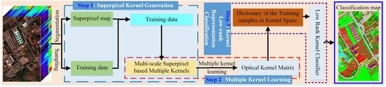
Figure 1 presents the architecture of proposed method, which is followed by detailed descriptions of each component.

2.1. Superpixel Kernel Generation

First, the PCA method is used to reduce the dimension of the hyperspectral data. Next, the ERS superpixel segmentation method [41] generates several superpixels in the first principal component image. Figure 2 shows the superpixel segmentation result of the Indian Pines dataset in which each successive neighborhood is a superpixel.

Assuming $x_i$ represents the $i$-th sample in the image and $x_{s{p}_i}$ represents the superpixel containing $x_i$, and $\varphi$ is a function mapping $x$ to the high-dimensional feature space to obtain the new feature $\varphi (x)$. The neighborhood information of $x_i$ in the kernel feature space is extracted by the mean filtering, which is defined as

$${\varphi }_{SPMF}(x_i)=\frac{1}{n_i}{\displaystyle \sum _{m=1}^{n_i}\varphi (x_{s{p}_i}^m)},m=1,2,\cdots ,n_i$$

(1)

where $n_i$ and $x_{s{p}_i}^m$ represent the number of pixels located in $x_{s{p}_i}$ and the $m$-th pixel in $x_{s{p}_i}$, respectively. The superpixel kernel between $x_i$ and $x_j$ can be represented as

$$K_{SPMF}^{\sigma }(x_i,x_j)=\langle {\varphi }_{SPMF}^{}(x_i),{\varphi }_{SPMF}^{}(x_j)\rangle$$

$$=\langle \frac{1}{n_i}{\displaystyle \sum _{m=1}^{n_i}\varphi (x_{s{p}_i}^m)},\frac{1}{n_j}{\displaystyle \sum _{m\prime =1}^{n_j}\varphi (x_{s{p}_i}^{m\prime })}\rangle$$

(2)

$$=\frac{1}{n_i{n}_j}{\displaystyle \sum _{m=1}^{n_i}{\displaystyle \sum _{m\prime =1}^{n_j}{K}^{\sigma }(x_{s{p}_i}^m,x_{s{p}_j}^{m\prime })}}$$

where $n_j$ is the number of pixels located in $x_{s{p}_j}$. $K^{\sigma }(x_{s{p}_i}^m,x_{s{p}_j}^{m\prime })=\exp (-{\Vert x_{s{p}_i}^m-x_{s{p}_j}^{m\prime }\Vert }^2/2{\sigma }^2)$ is the Gaussian RBF kernel function, and $\sigma$ is kernel scale.

Considering the training set $X=[x_1,x_2,\cdots ,x_t]\in {ℝ}^{b\times t}$ with $b$ bands and $t$ training samples, and a testing sample $y\in {ℝ}^{b\times 1}$, the column feature vector for training and testing samples can be given as,

$$K_{SPMF}^{\sigma }(X,X)=\left[\begin{array}{ccc}{K}_{SPMF}^{\sigma }(x_1,x_1)& \cdots & K_{SPMF}^{\sigma }(x_1,x_t)\\ ⋮& \ddots & ⋮\\ K_{SPMF}^{\sigma }(x_t,x_1)& \cdots & K_{SPMF}^{\sigma }(x_t,x_t)\end{array}\right]\in {ℝ}^{t\times t}$$

(3)

$$K_{SPMF}^{\sigma }(X,y)={\left[K_{SPMF}^{\sigma }(x_1,y),\cdots ,K_{SPMF}^{\sigma }(x_t,y)\right]}^T\in {ℝ}^t$$

(4)

From the above definitions, the superpixel kernel directly calculates the similarity between two pixels by averaging the pixels values in the kernel feature space within the corresponding superpixel. Thus, it eases the problem caused by window-based techniques, effectively overcomes the influence of outliers in superpixels and reflects the similarities between two superpixels in the kernel feature space other than the similarities between two vectors.

2.2. Multiple Kernel Learning

From Equations (3) and (4), columns of $K_{SPMF}^{\sigma }(X,X)$ and $K_{SPMF}^{\sigma }(X,y)$ can be viewed as new feature vectors that can be used for the pixel-based classifiers. However, the value of kernel scale $\sigma$ also affect the classification accuracy. In this subsection, the representative multiple kernel learning method is then utilized to determine the final multiple kernel learning expression by seeking the optimal low dimension representation in the original space, which is comprised of multiple basic kernel matrices in the superpixel. Given $f$ kernel scales, ${\sigma }_{\min }={\sigma }_1<\cdots <{\sigma }_f={\sigma }_{\max }$ within the range $[{\sigma }_{\min },{\sigma }_{\max }]$, the Gram matrixes $K_{SPMF}^{{\sigma }_i}$, $i=1,2,\cdots ,f$, of the essential kernel function are computed using Equation (3), and each matrix is transformed to a column vector according to a fixed order obtaining a new expression in the form of $f$ kernel matrixes, $H_{SPMF}={[vec(K_{SPMF}^{{\sigma }_1}),vec(K_{SPMF}^{{\sigma }_2}),\cdots ,vec(K_{SPMF}^{{\sigma }_f})]}^T\in {ℝ}^{f\times t^2}$. Here, $vec(·)$ is a stacking operator that turns a matrix into a vector.

According to Reference [38], the following model is established to find the low-dimensional linear subspaces in the kernel matrix group:

$$\ell (W,Z)={\Vert H_{SPMF}-WZ\Vert }_F^2$$

(5)

where $W\in {ℝ}^{f\times p}$ is a matrix space after feature mapping as well as a linear space formed by its column vector ${\left\{w_r\right\}}_{r=1}^p$. $Z\in {ℝ}^{p\times t^2}$ is the projected matrix onto the linear subspace spanned by $W$.

The dual form of minimizing Equation (5) regard to $W$ is given as

$$\underset{W}{\arg \max }{\Vert W^T{\displaystyle {\sum }_{H_{SPMF}}W}\Vert }_F=\underset{W}{\arg \max }{\Vert W^T{H}_{SPMF}\Vert }_F$$

(6)

$$\mathrm{s}.\mathrm{t}.W^{T}W=I_p,$$

where ${\displaystyle {\sum }_{H_{SPMF}}=}{H}_{SPMF}{H}_{SPMF}{}^T$ and $I_p$ is the identity matrix with size $p\times p$.

The optimization of Equations (5) and (6) is solved by eigenvalue decomposition or singular value decomposition. By searching the $W^{*}$, the variances of $Z$ will be maximized. Using the same strategy in [38], we only take max-variance projection vector into account and set $p=1$. Then, the projection vector $W^{*}={[w_{11}^{*},\cdots ,w_{1f}^{*}]}^T$ is obtained. Here, $W^{*}$ represents the optimal weight vector of the kernel function, and the optimal kernel function is a linear combination of these weights, such as

$$K^{*}={\displaystyle \sum _{i=1}^f{w}_{1i}^{*}{K}^{{\sigma }_i}}$$

(7)

Finally, the optimal superpixel kernel in Equation (2) is formulated as

$$K_{{}_{SPMF}}^{*}(x_i,x_j)=\frac{1}{n_i{n}_j}{\displaystyle \sum _{m=1}^{n_i}{\displaystyle \sum _{m\prime =1}^{n_j}{K}^{*}(x_{s{p}_i}^m,x_{s{p}_j}^{m\prime })}}$$

(8)

The procedure for the superpixel multiple kernel learning method is outlined in Algorithm 1.

Algorithm 1. Superpixel multiple kernel learning (Sp_MKL)

Step 1: Inputs：training dataset $X$ and corresponding labels $l(X)$. Step 2: Give the range of kernel scale values $[{\sigma }_{\min },{\sigma }_{\max }]$. Step 3: Select $f$ scales: ${\sigma }_{\min }={\sigma }_1<\cdots <{\sigma }_f={\sigma }_{\max }$ using the KA method. Step 4: Compute $f$ superpixel kernel matrices using Equation (2). Step 5: Transform the superpixel kernel matrices to vectors and use Equation (6) to determine the optimal   weights $W^{*}={[w_{11}^{*},\cdots ,w_{1f}^{*}]}^T$. Step 6: Compute the optimal superpixel kernel functions using Equation (8).

2.3. Superpixel Kernel Low Rank Representation Classifier

In HSIs, the spectral characteristics of the homogeneous region are also changed because of the light, environment, weather, and other factors. The spectrums of pixels belonging to the same class may also be similar or different. This phenomenon of inconsistency decreases the classification accuracy. To solve this problem, it is necessary to excavate the characteristics of the spectral kernel space in HSIs and to build a more robust classification model using structured prior. In Reference [42], low rank representation was employed for HSI classification resulting in smooth boundaries between different classes in HSIs. Compared with other sparse prior based methods, the effect becomes more apparent within a much larger homogeneous region. Inspired by References [42,43,44], the superpixel kernel is applied to the low rank representation model for HSI classification. Specifically, a combination of the smooth slicing effect of low rank representation, the spatial information, and high-dimensional separability constructed by the superpixel kernel is made to improve the classification accuracy further.

Let $Y=[y_1,y_2,\mathrm{\dots },y_r]\in {ℝ}^{n\times r}$ be the testing sample set with $b$ bands and $r$ samples. We use the superpixel mapping function ${\varphi }_{SPMF}$ to map testing sample set $Y$ and training sample set $X=[x_1,x_2,\cdots ,x_t]\in {ℝ}^{b\times t}$ to high-dimensional space, that is,

$${\varphi }_{SPMF}(Y)={\varphi }_{SPMF}([y_1,y_2,\mathrm{\dots },y_r])=[{\varphi }_{SPMF}(y_1),{\varphi }_{SPMF}(y_2),\mathrm{\dots },{\varphi }_{SPMF}(y_r)],$$

$${\varphi }_{SPMF}(X)={\varphi }_{SPMF}([x_1,x_2,\cdots ,x_t])=[{\varphi }_{SPMF}(x_1),{\varphi }_{SPMF}(x_2),\mathrm{\dots },{\varphi }_{SPMF}(x_t)],$$

where $y_i,i=1,2,\cdots ,r$ represents the $i$-th testing sample, $x_i，i=1,2,\cdots ,t$ represents the $i$-th training sample.

Having these definitions in mind, the low rank representation-based classification is given as

$$\underset{U}{\arg \min }\frac{1}{2}{\Vert {\varphi }_{SPMF}(Y)-{\varphi }_{SPMF}(X)U\Vert }_F^2+\lambda {\Vert U\Vert }_{*},$$

(9)

where $U$ is an unknown low rank coefficient matrix and $\lambda$ is a regulatory factor. A lower value of $\lambda$ indicates a weaker constraint on the rank of $U$.

After solving $U$, the classification criteria based on the kernel low rank can be defined as

$$class(y_i)=\underset{c=1,2,\cdots ,C}{\arg \min }{\Vert {\varphi }_{SPMF}(y_i)-{\varphi }_{SPMF}(X){\delta }_c(U_i)\Vert }_F^2,$$

(10)

where $c=\{1,2,\cdots ,C\}$ is a category index of a pixel, and ${\delta }_c(U_i)$ is an indicator operation zeroing out all elements of $y_i$ that do not belong to the class $c$.

Having $K(X,X)={\varphi }_{SPMF}{(X)}^T{\varphi }_{SPMF}(X)$, all high-dimensional mappings in Equation (9) are expressed in the form of an inner product as

$$\underset{U}{\arg \min }\frac{1}{2}Tr(U^{T}GU)-Tr(U^{T}P)+\lambda {\Vert U\Vert }_{*}+const,$$

(11)

where $const$ is a constant term, $G$ is a positive semi-definite matrix with elements $G_{ij}=K_{{}_{SPMF}}^{*}(x_i,x_j)$. $P$ is a matrix with elements $P_{ij}=K_{{}_{SPMF}}^{*}(x_i,y_j)$. Thus, the classification criteria is rewritten as

$$class(y_i)=\underset{c=1,2,\cdots ,C}{\arg \min }{\delta }_c^T(U_i)G{\delta }_c(U_i)-2{\delta }_c^T(U_i)P$$

(12)

The optimization of Equation (11) is a convex problem solvable using ADMM [45]. Substituting $U$ with variable $V$, Equation (11) is transmuted into the constrained optimization problem as

$$\underset{U}{\arg \min }\frac{1}{2}Tr(U^{T}GU)-Tr(U^{T}P)+\lambda {\Vert V\Vert }_{*}\mathrm{s}.\mathrm{t}.V=U.$$

(13)

Using the Lagrange multiplier method to transform Equation (13) into an unconstrained optimization problem, we obtain the following expression:

$$(U,V)=\underset{U,V}{\arg \min }\frac{1}{2}Tr(U^{T}GU)-Tr(U^{T}P)+\lambda {\Vert V\Vert }_{*}+Tr(L^T(U-V)+\frac{\mu }{2}{\Vert U-V\Vert }_F^2),$$

(14)

$$L=L+\mu (U-V),$$

(15)

where $L$ is the Lagrangian multiplier and $\mu$ is the Lagrangian parameter.

ADMM adopts an alternately updating variables strategy to solve the above optimization with

$$\begin{gathered} V^{*}=\underset{V}{\arg \min }\lambda {\Vert V\Vert }_{*}+Tr(L^T(U-V)+\frac{\mu }{2}{\Vert U-V\Vert }_F^2) \\ =\underset{V}{\arg \min }\frac{2\lambda }{\mu }{\Vert V\Vert }_{*}+({\Vert V-U-L/\mu \Vert }_F^2), \end{gathered}$$

(16)

$$U^{*}=\underset{U,V}{\min }\frac{1}{2}Tr(U^{T}GU)-Tr(U^{T}P)+Tr(L^T(U-V)+\frac{\mu }{2}{\Vert U-V\Vert }_F^2)$$

(17)

The optimum solution of Equation (16) is then formulated as:

$$V^{*}=T_{2\lambda /\mu }(U+L/\mu )=A{\mathsf{\Theta }}_{2\lambda /\mu }(\Sigma )B^T,$$

(18)

where $A(\Sigma )B^T$ is the singular value decomposition of the matrix $V+L/\mu$ and ${\mathsf{\Theta }}_{2\lambda /\mu }$ is a soft threshold operator: ${\mathsf{\Theta }}_{2\lambda /\mu }(x)=\mathrm{sgn}(x)\max (|x|-2\lambda /\mu ,0)$.

The optimization problem of Equation (17) has an explicit solution of the following equation:

$$U^{*}={(G+\mu I)}^{-1}(P+\mu (V-\frac{L}{\mu }))$$

(19)

In Equations (14)–(19), $\mu$ is a penalty parameter. A dynamic update strategy is applied to accelerate the speed of iteration with the equation:

$${\mu }^{k+1}=\{\begin{array}{cc}\rho {\mu }^k,& if{\mu }^k\max \{\Vert U^{k+1}-U^k\Vert ,\Vert V^{k+1}-V^k\Vert \}\le {\epsilon }_1\\ {\mu }^k,& otherwise\end{array}$$

(20)

where $\rho \ge 1$ and $0\le {\epsilon }_1\le 1$. The iteration stopping condition is set as:

$$\{\begin{array}{c}\Vert U^{k+1}-V^{k+1}\Vert \le {\epsilon }_2\\ {\mu }^k\max \{\Vert U^{k+1}-U^k\Vert ,\Vert V^{k+1}-V^k\Vert \}\le {\epsilon }_1\end{array}$$

(21)

The process of the superpixel kernel and low rank representation-based classifier is provided in Algorithm 2.

Algorithm 2. Superpixel kernel low rank representation-based classification algorithm

Step 1: Inputs：training sample set $X$ and corresponding category set along with the testing sample set $Y$. Step 2: Select the optimal superpixel kernel function using Algorithm 1. Step 3: Calculate $G$ ($G_{ij}=K_{SPMF}^{*}(x_i,x_j)$) and $P$ ($P_{ij}=K_{SPMF}^{*}(x_i,y_j)$) using Equation (8). Step 4: Initialize $k=0$, $U^0=V^0=0$, $Y^0=0$, $\mu ={10}^{-6}$, ${\mu }^{\max }={10}^6$, and $\rho =1.1$. while not converged do   Step 5: Update $V^{k+1}=T_{2\lambda /\mu }(U^k+L^k/\mu )=A^k{\mathsf{\Theta }}_{2\lambda /{\mu }^k}({\Sigma }^k){(B^k)}^T$.   Step 6: Update $U^{k+1}={(G+{\mu }^{k}I)}^{-1}(P+{\mu }^k(V^k-L^k/{\mu }^k))$.   Step 7: Update $L^{k+1}=L^k+{\mu }^k(U^{k+1}-V^{k+1})$.   Step 8: Update the penalty factor $\mu$ with Equation (20).   Step 9: Calculate the iteration stopping condition according to Equation (21).   if $\Vert U^{k+1}-V^{k+1}\Vert \le {\epsilon }_2$ or ${\mu }^k\max \{\Vert U^{k+1}-U^k\Vert ,\Vert V^{k+1}-V^k\Vert \}\le {\epsilon }_1$    Break;   otherwise    Go to Step 5 and update $k=k+1$.   end end while Step 10: Determine the class of each pixel with Equation (12). Step 11: Output：the categories of testing samples.

3. Results

3.1. Datasets Description and Assessment Indicators

To verify the effectiveness of the proposed method, two real hyperspectral image datasets are employed for performance evaluation of classification. They are downloaded from http://lesun.weebly.com/hyperspectral-data-set.html. These two datasets have been well pre-processed. Therefore, we can mainly focus on the task of HSI classification. The only preprocessing applied to these two datasets is normalization.

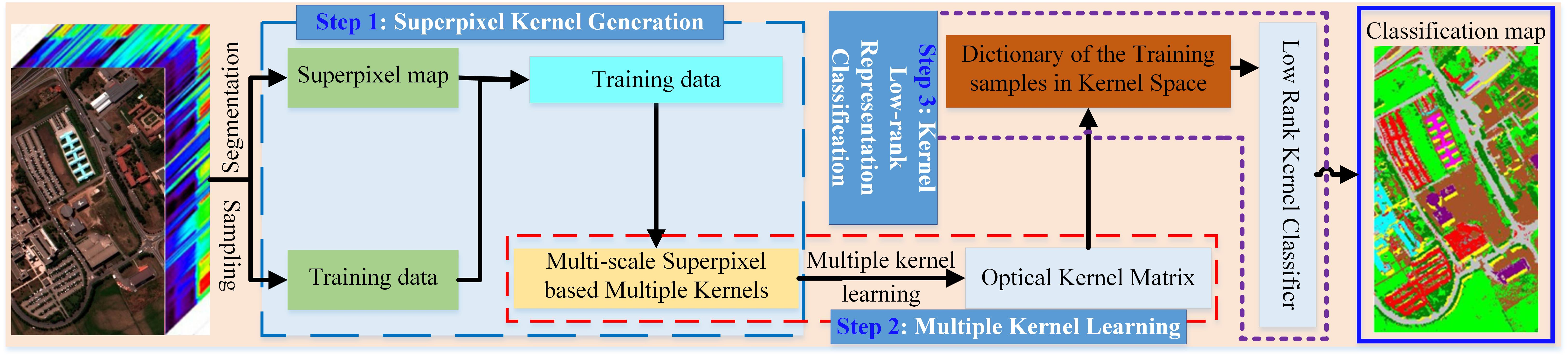
Indian Pines Data: This dataset was collected by the airborne visible light/infrared imaging spectrometer (Airborne Visible Infrared Imaging Spectrometer, AVIRIS) over the Indian Pine test site in Northwest Indiana, USA. The spatial size of the image is 145 × 145 pixels and the spatial resolution is 20 m/pixel. The original dataset contains 224 bands across the spectral range from 0.2 to 2.4 µm. In this experiment, 4 bands full of zero and 20 water vapor absorption bands are removed with the remaining 200 bands used for classification. Figure 3a shows a pseudo color image; moreover, Figure 3b shows the corresponding ground truth, that contains sixteen types of objects.

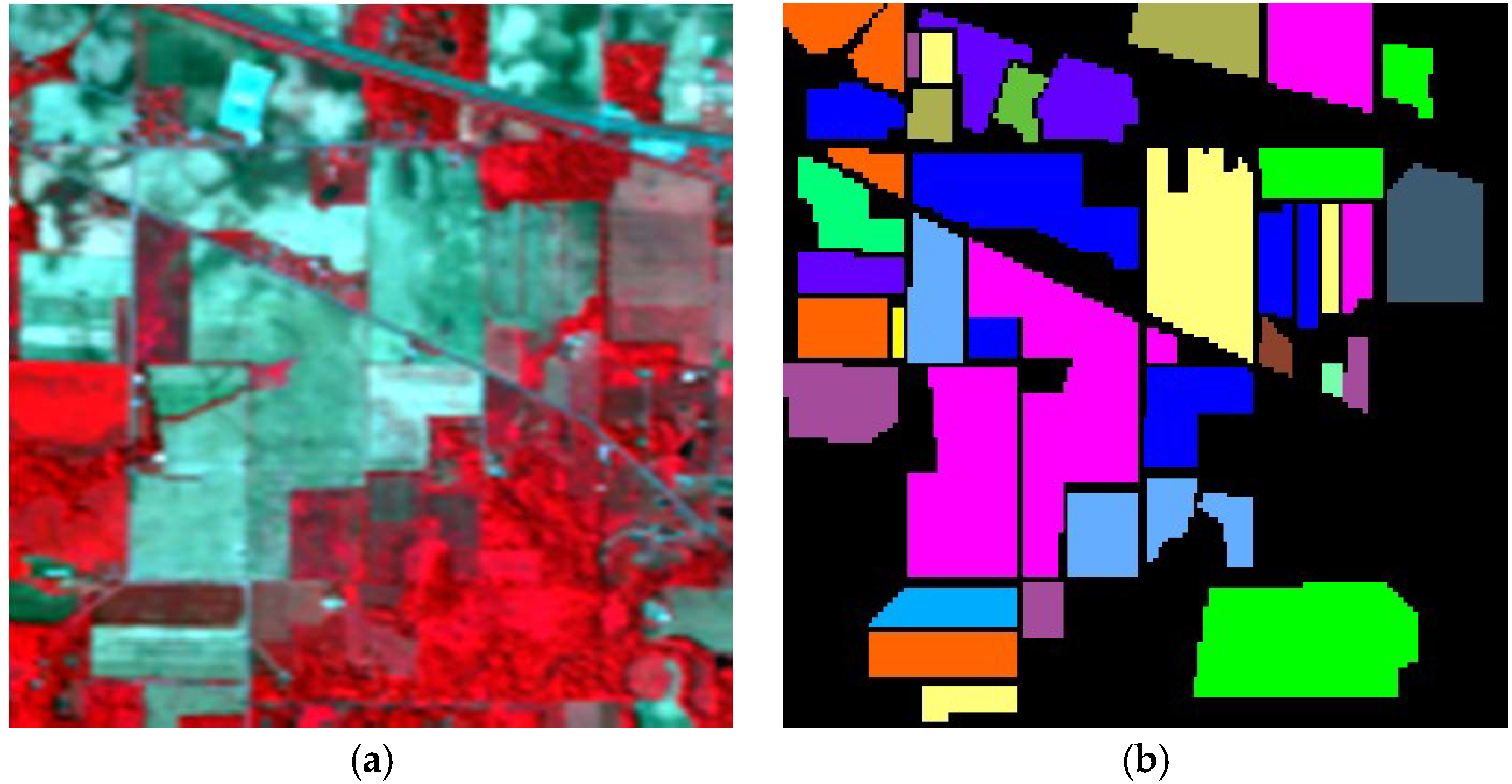
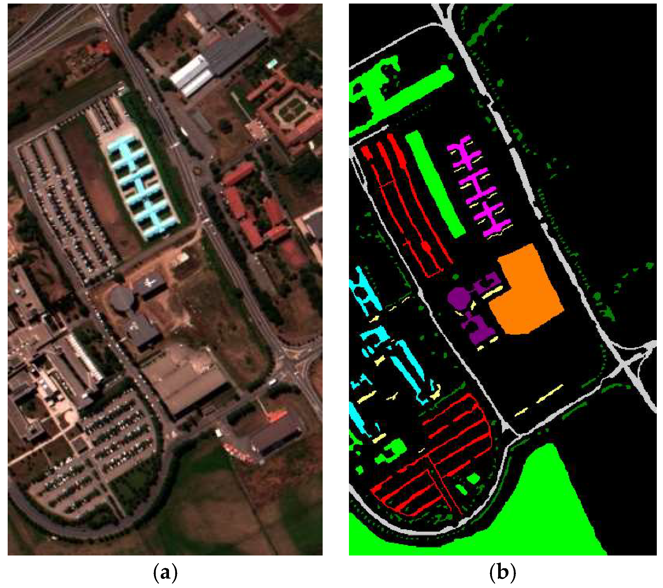
University of Pavia: This dataset was collected by the Reflective Optics System Imaging Spectrometer optical sensor (ROSIS) over an urban area surrounding the University of Pavia. The spatial size of the image is 610 × 340 and the spatial resolution is 1.3 m per pixel. The original dataset contains 115 bands across the spectral range from 0.43 to 0.86 µm. After removing 12 noisy bands, 103 bands remain for classification. Figure 4a shows its false color image and Figure 4b shows the corresponding ground truth, which contains nine types of objects.

Experiments have been carried out to compare the HSI classification with several methods, including the proposed Sp_MKL_LRR method, the traditional classifiers (e.g., SVM and LRR), spectral-spatial combined method (e.g., SMLR_SPTV), the kernel based method (e.g., SVMCK), the superpixel based methods (e.g., SPCK, SCMK) and multiple kernel learning method (e.g., RMLK). The simple definitions of these methods are given as follows:

(1)

SVM: Support vector marching-based classifier [46];

(2)

LRR: Low rank representation-based classifier [44];

(3)

SVMCK: Composite kernels and SVM-based method [32];

(4)

SMLR_SPTV: Multinomial logistic regression and spatially adaptive total variation based method [26];

(5)

SPCK: Superpixel based composite kernel and SVM classifier [37];

(6)

SCMK: Superpixel, multiple kernels and SVM-based method [42];

(7)

RMKL: Representative multiple kernel learning and SVM-based method [38];

(8)

Sp_MKL_SVM: The proposed superpixel multiple kernel learning and SVM-based method;

(9)

Sp_MKL_LRR: The proposed method.

The overall accuracy (OA), average accuracy (AA), and the kappa ($\kappa$) coefficient are used as key properties of performances evaluation. Assuming that a confusion matrix with $C$ classes is denoted by $M$, in which the matrix element $M_{ij}$ represents the sample amount of the $i$-th class that is classified as the $j$-th class. The expressions of OA, AA and $\kappa$ are given as follows:

$$\begin{gathered} \mathrm{OA}={\displaystyle \sum _{i=1}^C{M}_{ii}/r}, \\ \mathrm{AA}=\frac{1}{C}{\displaystyle \sum _{i=1}^C{(M_{ii}/r}_i)}, \\ \kappa =(r({\displaystyle \sum _{i=1}^C{M}_{ii}})-{\displaystyle \sum _{i=1}^C({\displaystyle \sum _{j=1}^C{M}_{ij}}{\displaystyle \sum _{j=1}^C{M}_{ji}})})/(r^2-{\displaystyle \sum _{i=1}^C({\displaystyle \sum _{j=1}^C{M}_{ij}}{\displaystyle \sum _{j=1}^C{M}_{ji}})}), \end{gathered}$$

where, $r$ is the number of all testing samples and $r_i$ is the number of testing samples in $i$-th class.

The experimental results are calculated by averaging the values obtained after ten Monte Carlo runs.

3.2. Parameters Analysis

3.2.1. The Number of Superpixels

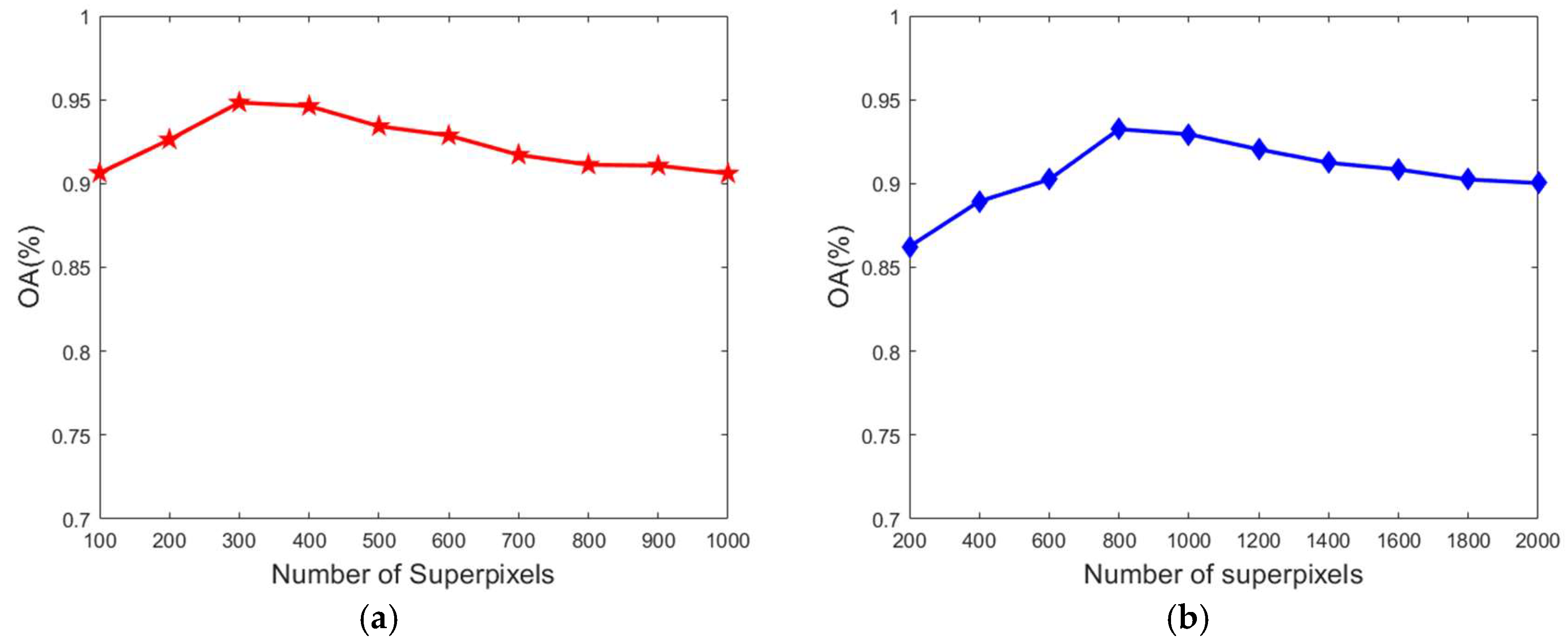
Different numbers of superpixels are used in the proposed method to study its influence on HSI classification accuracy. As a result, Figure 5 shows the OA values obtained from the proposed method based on two datasets. From these results, it is obvious that the classification results have poor performance when the scale of superpixel amount is extremely large or small. Such inferior performance is caused by the superpixel containing pixels from different substances in the condition of very large-scale of superpixel amount and even larger homogeneous. Conversely, in the condition of extremely small-scale amount of superpixels, the performance of the spatial constraint degrades and leads to a lower classification accuracy. In the experiments, the proposed method achieves better classification performance when the number of superpixels ranging in (200, 500) for the Indian Pines dataset and [600, 1600] for the University of Pavia dataset with an optimal number of superpixels of 300 and 800, respectively.

3.2.2. Impact of Parameter $\lambda$

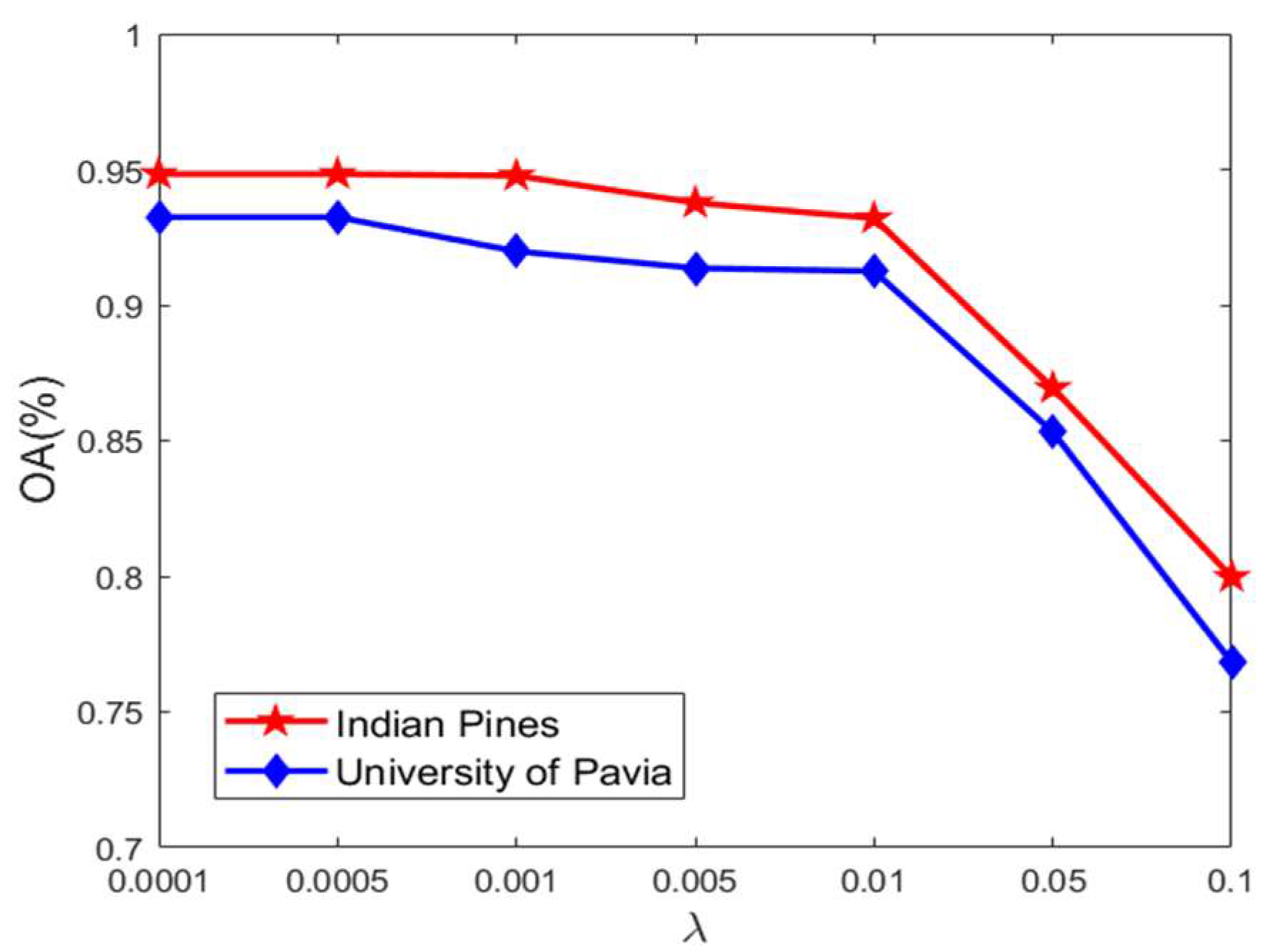
Figure 6 plots the OA results as a function of the parameter $\lambda$ from Equation (7) based on the Indian Pines and University of Pavia datasets. From the results, the best classification performance is obtained when the value of $\lambda$ is in the range of [0.0001, 0.001]. The OA value reduces rapidly after the value of $\lambda$ growing over 0.001. This is caused by the fact that the low rank constraint performance is stronger when a large value is set for $\lambda$. It also affects the similarity of the first half of Equation (9) and forces the pixels belonging to different categories to be classified into the same category with such a strong low rank constraint. In the experiments, the value of $\lambda$ is set to 0.0001.

3.2.3. Impact of the Number of Training Samples

Figure 7 shows the classification accuracy of the proposed method and the superpixel multiple kernel learning-based SVM classifier (Sp_MKL_SVM) which is obtained on a different number of training samples. The Sp_MKL_SVM classifier is generated by the SVM classifier to replace the low rank representation classifier in the Sp_MKL_LRR classifier. From these results, the classification accuracy of the Sp_MKL_SVM method depends on the number of training samples in more depth. Compared with Sp_MKL_SVM, the proposed method offers better classification accuracy with fewer training samples. The classification accuracy is more stable when more than 3% and 15% samples are selected as training samples from the Indian Pines and University of Pavia datasets, respectively. The comparison results show that the low rank representation method obtains better classification results when the training set is small.

3.3. Classification Results on AVIRIS Indian Pines Dataset

Figure 8 shows the classification results using different methods on the Indian Pines dataset. The corresponding OA, AA, and kappa coefficient are included in

Table 1. The classification results on Indian Pines dataset.

Class	Methods
	SVM	LRR	SVMCK [32]	SMLR_SPTV [26]	SPCK [37]	SCMK [42]	RMKL [38]	Sp_MKL_SVM	Sp_MKL_LRR
Alfalfa	0.446	0.824	0.445	0.565	0.829	0.963	0.659	0.86	1
Corn-no till	0.763	0.766	0.844	0.9	0.905	0.884	0.847	0.884	0.971
Corn-min till	0.662	0.713	0.833	0.836	0.919	0.892	0.76	0.929	0.996
Corn	0.604	0.882	0.659	0.794	0.792	0.774	0.667	0.833	0.956
Grass-pasture	0.903	0.914	0.853	0.851	0.893	0.905	0.944	0.836	0.817
Grass-trees	0.951	0.956	0.947	0.978	0.974	0.953	0.957	0.925	0.978
Grass-pasture-mowed	0	0.824	0.586	0.8	0.776	0.736	0.941	0.736	1
Hay-windrowed	0.993	0.99	0.973	1	0.987	0.987	0.996	0.984	0.998
Oats	0	0.333	0.711	0	0.979	0.995	0.125	0.7	0.842
Soybean-no till	0.566	0.596	0.801	0.835	0.814	0.913	0.726	0.891	0.978
Soybean-min till	0.822	0.842	0.867	0.969	0.913	0.944	0.851	0.972	0.992
Soybean-clean till	0.751	0.769	0.752	0.861	0.815	0.769	0.89	0.919	0.84
Wheat	0.984	0.994	0.941	0.995	0.995	0.989	0.99	0.986	0.942
Woods	0.965	0.962	0.848	0.985	0.965	0.987	0.967	0.979	0.998
Buildings-grass-trees	0.571	0.648	0.673	0.741	0.771	0.88	0.614	0.934	0.989
Stone-still-towers	0.817	0.923	0.933	0.571	0.989	0.899	0.933	0.903	1
OA	0.797	0.823	0.856	0.907	0.905	0.919	0.856	0.931	0.969
AA	0.677	0.809	0.798	0.895	0.895	0.904	0.804	0.892	0.956
Kappa	0.767	0.797	0.835	0.891	0.891	0.907	0.835	0.921	0.964

. The classification accuracy of the SVM classifier is much lower when using fewer training samples. The accuracy of the LRR classifier is much higher than that of the SVM classifier, which demonstrates that the LRR classifier can ensure better classification accuracy with fewer training samples. In the SVMCK method, the square window is used to select the homogeneous region, so the classification accuracy is not satisfactory. The SMLR_SpTV method used the MRF regular term of the TV first-order neighborhood system to describe the spatial information. Although the effect is good at the edge region in the image, the classification accuracy within the small regions is very low. Compared with SVMCK, the SPCK method using a superpixel to select homogeneous regions improves the classification accuracy of the edge pixels significantly. SCMK utilized the multiple kernel technique to improve the accuracy of its classification further. MKL_LRR is a multiple kernel learning-based low rank representation method, which has a higher classification accuracy in small object areas compared with the SCMK method. Sp_MKL_SVM is a method combining superpixel multiple kernel learning and SVM classification with an overall classification precision higher than that of the previous methods. The proposed Sp_MKL_LRR method provides the highest classification accuracy, especially for small objects, because it integrates the advantages of the superpixel kernel, multiple kernel learning, and low rank representation in HSI classification.

3.4. Classification Results on ROSIS University of Pavia Dataset

In this experiment, the proposed method is evaluated with the ROSIS University of Pavia data set while comparing with other state-of-the-art methods mentioned above. Figure 9 shows the classification results using different methods on the ROSIS University of Pavia dataset. The corresponding OA, AA, and kappa coefficient are included in

Table 2. The classification results on University of Pavia dataset.

Class	Methods
	SVM	LRR	SVMCK [32]	SMLR_SPTV [26]	SPCK [37]	SCMK [42]	RMKL [38]	Sp_MKL_SVM	Sp_MKL_LRR
Asphalt	0.7285	0.7026	0.8579	0.8478	0.8683	0.8213	0.7849	0.8037	0.8645
Meadows	0.6124	0.7704	0.8684	0.8873	0.8598	0.8803	0.8366	0.8763	0.9843
Gravel	0.633	0.7744	0.8402	0.8351	0.9012	0.9542	0.7519	0.9619	0.9981
Tress	0.953	0.9484	0.9233	0.8785	0.9612	0.9587	0.9295	0.7699	0.8233
Metal sheets	0.9894	0.9936	0.9913	0.9974	0.9798	0.9965	0.9936	0.9713	1
Bare soil	0.682	0.7277	0.8283	0.933	0.7849	0.8717	0.8174	0.9444	0.9241
Bitumen	0.8168	0.8659	0.9303	0.9977	0.9454	0.9378	0.8894	0.9897	1
Bricks	0.8258	0.6625	0.7384	0.9054	0.8581	0.87	0.7582	0.951	0.9629
Shadows	0.9666	0.9858	0.9943	0.3147	0.9837	0.9884	0.9988	0.99	0.6268
OA	0.708	0.7722	0.8619	0.8793	0.8705	0.8862	0.8316	0.885	0.9391
AA	0.8088	0.8257	0.8859	0.8441	0.9048	0.9199	0.8623	0.9176	0.9093
Kappa	0.6369	0.7068	0.8208	0.8435	0.8325	0.8523	0.781	0.8519	0.9192

. As concluded previously, the proposed Sp_MKL_LRR classifier achieves the highest accuracy among all the other classifiers. The results here also show that the proposed method can obtain better classification performance on irregularly shaped regions by using the superpixel kernel method. A kernel-based low rank classifier can also obtain better classification results on small object areas with fewer training samples. Meanwhile, the multiple kernel learning overcomes the single feature scale issue and difficult parameter determination of the kernel methods. All these advantages lead to the proposed method achieving the highest classification accuracy among all the reviewed classifiers.

4. Discussion

The airborne or space-borne hyperspectral sensors collect data in hundreds of adjacent narrow spectral bands. The differences of their spectral features provide a great important significance to conduct different materials classification. In the last decade, several HSI classification methods were proposed for improving the classification performance. In this paper, we proposed a novel superpixel kernel learning based low rank representation method for HSI classification. During this study, we find that the classification effect obtained by integrating spatial information in the classification process is better than those methods without spatial information, and the superpixel can well introduce spatial information. The kernel-based methods transform the linearly non-separable high-dimensional data to be linearly separable by mapping the data to the higher dimensional nonlinear feature space. Thus, the kernel-based methods are able to improve HSI classification accuracy further. Compared with the single kernel-based method, these multiple kernel-based methods are more conducive to enhance the interpretability of decision functions and to represent the properties of the original sample space fully. In this paper, the KA criterion is applied to find the optimal kernel function, thus effectively solves the problem of kernel selection. In the classifier design process, we use low rank representation classifier to execute HSI classification task. The experimental results on two datasets demonstrate that the classification performance of the low rank representation classifier is better than that of SVM classifier and MLR classifier. Moreover, the number of training samples required by the low rank classifier is not as strict as that of the other classifiers.

There are three parameters in the proposed Sp_MKL_LRR method. The first one is the number of superpixels. We find that the classification accuracy is not satisfactory when the number of superpixels is either in an extremely large-scale or in an extremely small-scale. The capacity of spatial constraint will be affected when the number of superpixels is too much, and the purity of a single superpixel will be reduced if the number of superpixel is too little. From the experimental results, we think that the choice of superpixel number in HSI image is related to the size and the content complexity of HSI image. The number of superpixels chosen between 0.3% and 0.5% of image size will deliver a good classification performance. It is also suggested that the number of superpixels can be reduced if the content of HSI image is relatively simple, and the number of superpixels should be increased if the content of HSI image is quite complex. The second parameter is $\lambda$ in low rank representation. This parameter is used to balance the class discrimination ability and low rank constraint. We suggest to take the value of $\lambda$ in the range of [0.0001, 0.001] when using the proposed KLRR method presented in Equation (7). The third parameter is the numbers of training samples. The experimental results show that the proposed method is not strict with the number of training samples. 15% of global samples in each class used for training is sufficient for obtaining an outstanding classification result. This demonstrates that the low rank representation-based classifier is robust to the number of training samples.

Based on the above analysis and discussion, the future work will focus on multi-scale superpixels fusion for HSI classification, automatic selection of parameter in LRR classifier and high-performance computing. We will continue to improve the efficiency of the proposed method to meet the practical application of massive hyperspectral imagery.

5. Conclusions

A hyperspectral classification method is proposed, which is designed on the basis of a superpixel kernel, multiple kernel learning, and low rank representation. With this method, we first construct superpixel graphics and select homogeneous regions for dimensionality reduction results on hyperspectral images. Second, according to the multiple kernel learning framework, an optimal superpixel kernel function is selected through the feature of the superpixel kernel matrix. Finally, the optimal superpixel kernel and low rank representation classifier are integrated to execute HSI classification. The proposed method is applied to the Indian Pines and University of Pavia datasets. OA, AA, and the kappa coefficient obtained on two datasets are 0.9685, 0.9560, 0.9641 and 0.9391, 0.9093, 0.9192, respectively. Compared with SVM classifier, the OA, AA and the kappa coefficient obtained by the proposed method improved 16%, 27%, 20% on Indian Pines dataset and 14%, 15%, 17% on the University of Pavia dataset. Compared with LRR classifier, the OA, AA and the kappa coefficient obtained by the proposed method improved 14%, 15%, 17% on Indian Pines dataset and 16%, 8%, 21% on the University of Pavia dataset. Compared with other state-of-art methods, the OA, AA and the kappa coefficient obtained by the proposed method improved 5–11%, 5–16%, 7–13% on Indian Pines dataset and 5–10%, −0.1–6%, 6–13% on the University of Pavia dataset. These results demonstrate the superiority of the proposed method in HSI classification. At the same time, the proposed method obtains higher classification accuracy under a variety of conditions, such as fewer training samples, small object areas, and irregular regions.

References

- Carrino, T.A.; Crósta, A.P.; Toledo, C.L.B.; Silva, A.M. Hyperspectral remote sensing applied to mineral exploration in southern Peru: A multiple data integration approach in the Chapi Chiara gold prospect. Int. J. Appl. Earth Obs. Geoinf. 2018, 64, 287–300. [Google Scholar] [CrossRef]
- Adão, T.; Hruška, J.; Pádua, L.; Bessa, J.; Peres, E.; Morais, R.; Sousa, J.J. Hyperspectral Imaging: A review on UAV-based sensors, Data Processing and Applications for Agriculture and Forestry. Remote Sens. 2017, 9, 1110. [Google Scholar]
- Xu, Y.; Wu, Z.; Chanussot, J.; Wei, Z. Joint reconstruction and anomaly detection from compressive hyperspectral images using mahalanobis distance-regularized tensor RPCA. IEEE Trans. Geosci. Remote Sens. 2018, 56, 2919–2930. [Google Scholar] [CrossRef]
- Niu, Y.; Wang, B. Extracting target spectrum for hyperspectral target detection: an adaptive weighted learning method using a self-completed background dictionary. IEEE Trans. Geosci. Remote Sens. 2017, 55, 1604–1617. [Google Scholar] [CrossRef]
- Zhu, J.; Hu, J.; Jia, S.; Jia, X.; Li, Q. Multiple 3-D feature fusion framework for hyperspectral image classification. IEEE Trans. Geosci. Remote Sens. 2018, 56, 1873–1886. [Google Scholar] [CrossRef]
- Sun, L.; Jeon, B.; Soomro, B.N.; Zheng, Y.; Wu, Z.; Xiao, L. Fast superpixel based subspace low rank learning method for hyperspectral denoising. IEEE Access. 2018, 6, 12031–12043. [Google Scholar] [CrossRef]
- Jia, S.; Deng, B.; Zhu, J.; Jia, X.; Li, Q. Local binary pattern-based hyperspectral image classification with superpixel guidance. IEEE J. Sel. Top. Appl. Earth Obs. Remote Sens. 2018, 56, 749–759. [Google Scholar] [CrossRef]
- Sun, L.; Jeon, B.; Zheng, Y.; Wu, Z. A novel weighted cross total variation method for hyperspectral image mixed denoising. IEEE Access. 2017, 5, 27172–27188. [Google Scholar] [CrossRef]
- Gao, Q.; Lim, S.; Jia, X. Hyperspectral image classification using convolutional neural networks and multiple feature learning. Remote Sens. 2018, 10, 299. [Google Scholar] [CrossRef]
- Sun, L.; Jeon, B.; Zheng, Y.; Wu, Z. Hyperspectral image restoration by using low rank representation on spectral difference image. IEEE Geosci. Remote Sens. Lett. 2017, 14, 1115–1155. [Google Scholar] [CrossRef]
- Li, J.; Bioucas-Dias, J.M.; Plaza, A. Spectral–spatial hyperspectral image segmentation using subspace multinomial logistic regression and Markov random fields. IEEE Trans. Geosci. Remote Sens. 2012, 50, 809–823. [Google Scholar] [CrossRef]
- Wu, Y.; Yang, X.; Plaza, A.; Qiao, F.; Gao, L.; Zhang, B.; Cui, Y. Approximate computing of remotely sensed data: SVM Hyperspectral image classification as a case study. IEEE J. Sel. Top. Appl. Earth Obs. Remote Sens. 2017, 9, 5806–5818. [Google Scholar] [CrossRef]
- Yuan, H.; Yang, G.; Li, C.; Wang, Y.; Liu, J.; Yu, H.; Feng, H.; Xu, B.; Zhao, X.; Yang, X. Retrieving soybean leaf area index from unmanned aerial vehicle hyperspectral remote sensing: analysis of RF, ANN, and SVM regression models. Remote Sens. 2017, 9, 309. [Google Scholar] [CrossRef]
- Chang, C.I. Recursive Hyperspectral sample processing of maximum likelihood estimation. In Real-Time Recursive Hyperspectral Sample and Band Processing; Springer International Publishing: New York, NY, USA, 2017; pp. 289–317. [Google Scholar]
- Wu, Z.; Wang, Q.; Plaza, A.; Li, J.; Sun, L.; Wei, Z. Parallel implementation of sparse representation classifiers for hyperspectral imagery on GPUs. IEEE J. Sel. Top. Appl. Earth Obs. Remote Sens. 2015, 8, 2912–2925. [Google Scholar] [CrossRef]
- Sun, L.; Wang, S.; Wang, J.; Zheng, Y.; Jeon, B. Hyperspectral classification employing spatial–spectral low rank representation in hidden fields. J. Ambient Intell. Humaniz. Comput. 2017, 1–12. [Google Scholar] [CrossRef]
- Xu, Y.; Wu, Z.; Wei, Z. Spectral–spatial classification of hyperspectral image based on low-rank decomposition. IEEE J. Sel. Top. Appl. Earth Obs. Remote Sens. 2015, 8, 2370–2380. [Google Scholar] [CrossRef]
- Chen, C.; Li, W.; Su, H.; Liu, K. Spectral-spatial classification of hyperspectral image based on kernel extreme learning machine. Remote Sens. 2014, 6, 5795–5814. [Google Scholar] [CrossRef]
- Chen, Y.; Lin, Z.; Zhao, X.; Wang, G.; Gu, Y. Deep learning-based classification of hyperspectral data. IEEE J. Sel. Top. Appl. Earth Obs. Remote Sens. 2017, 7, 2094–2107. [Google Scholar] [CrossRef]
- He, L.; Li, J.; Plaza, A.; Li, Y. Discriminative low-rank Gabor filtering for spectral-spatial hyperspectral image classification. IEEE Trans. Geosci. Remote Sens. 2017, 55, 1381–1395. [Google Scholar] [CrossRef]
- Gan, L.; Du, P.; Xia, J.; Meng, Y. Kernel fused representation-based classifier for hyperspectral imagery. IEEE Geosci. Remote Sens. Lett. 2017, 14, 684–688. [Google Scholar] [CrossRef]
- Jia, S.; Deng, B.; Zhu, J.; Jia, X.; Li, Q. Superpixel-based multitask learning framework for hyperspectral image classification. IEEE Trans. Geosci. Remote Sens. 2017, 55, 2575–2588. [Google Scholar] [CrossRef]
- Moser, G.; Serpico, S.B. Combining Support vector machines and Markov random fields in an integrated framework for contextual image classification. IEEE Trans. Geosci. Remote Sens. 2013, 51, 2734–2752. [Google Scholar] [CrossRef]
- Zhang, H.; Li, J.; Huang, Y.; Zhang, L. A nonlocal weighted joint sparse representation classification method for hyperspectral imagery. IEEE J. Sel. Top. Appl. Earth Obs. Remote Sens. 2017, 7, 2056–2065. [Google Scholar] [CrossRef]
- Yuan, Y.; Lin, J.; Wang, Q. Hyperspectral image classification via multitask joint sparse representation and stepwise MRF optimization. IEEE Trans. Cybern. 2017, 46, 2966–2977. [Google Scholar] [CrossRef] [PubMed]
- Sun, L.; Wu, Z.; Liu, J.; Xiao, L.; Wei, Z. Supervised spectral–spatial hyperspectral image classification with weighted Markov random fields. IEEE Trans. Geosci. Remote Sens. 2015, 53, 1490–1503. [Google Scholar] [CrossRef]
- Luo, H.; Tang, Y.; Yang, X.; Yang, L.; Li, H. Autoencoder with extended morphological profile for hyperspectral image classification. In Proceeding of the 3rd IEEE International Conference on Cybernetics (CYBCONF 2017), Exeter, UK, 21–23 June 2017; pp. 1–4. [Google Scholar]
- Gu, Y.; Liu, T.; Jia, X.; Benediktsson, J.; Chanussot, J. Nonlinear multiple kernel learning with multiple-structure-element extended morphological profiles for hyperspectral image classification. IEEE Trans. Geosci. Remote Sens. 2016, 54, 3235–3247. [Google Scholar] [CrossRef]
- Makantasis, K.; Doulamis, A.D.; Doulamis, N.D.; Nikitakis, A. Tensor-based classification models for hyperspectral data analysis. IEEE Trans. Geosci. Remote Sens. 2018. [Google Scholar] [CrossRef]
- Zhang, L.; Zhang, L.; Tao, D.; Huang, X. Tensor discriminative locality alignment for hyperspectral image spectral–spatial feature extraction. IEEE Trans. Geosci. Remote Sens. 2013, 51, 242–256. [Google Scholar] [CrossRef]
- Guo, X.; Huang, X.; Zhang, L.; Zhang, L.; Plaza, A.; Benediktsson, J.A. Support tensor machines for classification of hyperspectral remote sensing imagery. IEEE Trans. Geosci. Remote Sens. 2016, 54, 3248–3264. [Google Scholar] [CrossRef]
- Camps-Valls, G.; Gomez-Chova, L.; Munoz-Mari, J.; Vila-France, J.; Calpe-Maravilla, J. Composite kernels for hyperspectral image classification. IEEE Geosci. Remote Sens. Lett. 2006, 3, 93–97. [Google Scholar] [CrossRef]
- Li, J.; Marpu, P.; Plaza, A.; Bioucas-Dias, J.; Benediktsson, J. Generalized composite kernel framework for hyperspectral image classification. IEEE Trans. Geosci. Remote Sens. 2013, 51, 4816–4829. [Google Scholar] [CrossRef]
- Liu, J.; Wu, Z.; Wei, Z.; Xiao, L.; Sun, L. Spatial-spectral kernel sparse representation for hyperspectral image classification. IEEE J. Sel. Top. Appl. Earth Obs. Remote Sens. 2013, 6, 2462–2471. [Google Scholar] [CrossRef]
- Li, S.; Lu, T.; Fang, L.; Jia, X.; Benediktsson, J. Probabilistic fusion of pixel-level and superpixel-level hyperspectral image classification. IEEE Trans. Geosci. Remote Sens. 2016, 4, 7416–7420. [Google Scholar] [CrossRef]
- Zhang, G.; Jia, X.; Hu, J. Superpixel-based graphical model for remote sensing image mapping. IEEE Trans. Geosci. Remote Sens. 2015, 53, 5861–5871. [Google Scholar] [CrossRef]
- Duan, W.; Li, S.; Fang, L. Superpixel-based composite kernel for hyperspectral image classification. In Proceeding of the IEEE International Geoscience and Remote Sensing Symposium (IGARSS 2015), Millan, Italy, 26–31 July 2015; pp. 1698–1701. [Google Scholar]
- Gu, Y.; Wang, C.; You, D.; Zhang, Y.; Wang, S.; Zhang, Y. Representative multiple kernel learning for classification in hyperspectral imagery. IEEE Trans. Geosci. Remote Sens. 2012, 50, 2852–2865. [Google Scholar] [CrossRef]
- Gu, Y.; Chanussot, J.; Jia, X.; Benediktsson, J. Multiple kernel learning for hyperspectral image classification: A review. IEEE Trans. Geosci. Remote Sens. 2017, 55, 6547–6565. [Google Scholar] [CrossRef]
- Bajorski, P. Statistical inference in PCA for hyperspectral images. IEEE J. Sel. Top. Signal Process. 2011, 5, 438–445. [Google Scholar] [CrossRef]
- Liu, M.; Tuzel, O.; Ramalingam, S.; Chellappa, R. Entropy rate superpixel segmentation. In Proceedings of the Computer Vision and Pattern Recognition, Colorado Springs, CO, USA, 20–25 June 2011; IEEE: Piscataway, NJ, USA; pp. 2097–2104. [Google Scholar]
- Du, L.; Wu, Z.; Xu, Y.; Liu, W.; Wei, Z. Kernel low-rank representation for hyperspectral image classification. In Proceedings of the 2016 IEEE International Geoscience and Remote Sensing Symposium, Beijing, China, 10–15 July 2016; IEEE: Piscataway, NJ, USA; pp. 477–480. [Google Scholar]
- Fang, L.; Li, S.; Duan, W.; Ren, J.; Benediktsson, J. Classification of hyperspectral images by exploiting spectral–spatial information of superpixel via multiple kernels. IEEE Trans. Geosci. Remote Sens. 2015, 53, 6663–6674. [Google Scholar] [CrossRef]
- Liu, G.; Lin, Z.; Yan, S.; Sun, J.; Yu, Y.; Ma, Y. Robust recovery of subspace structures by low-rank representation. IEEE Trans. Pattern Anal. Machi. Intell. 2010, 35, 171–184. [Google Scholar] [CrossRef] [PubMed]
- Boyd, S.; Parikh, N.; Chu, E.; Peleato, B.; Eckstein, J. Distributed optimization and statistical learning via the alternating direction method of multipliers. Found. Trends Mach. Learn. 2010, 3, 1–122. [Google Scholar] [CrossRef]
- Chang, C.C.; Lin, C.J. LIBSVM: a library for support vector machines. ACM Trans. Intell. Systems Technol. 2011, 2, 1–27. [Google Scholar] [CrossRef]
Figure 1.
The overflow of the proposed Sp_MKL_LRR method.
Figure 2.
The superpixel segmentation of the Indian Pines dataset.
Figure 3.
(a) false color map and (b) ground truth of the Indian Pines dataset.
Figure 4.
(a) false color map and (b) ground truth of the University of Pavia dataset.
Figure 5.
Classification performances from different numbers of superpixels for (a) the Indian Pines and (b) University of Pavia datasets.
Figure 6.
Impact of the low rank constraint parameter .
Figure 7.
Impact of the number of training samples. (a) Indian Pines dataset and (b) University of Pavia dataset.
Figure 8.
Indian Pines dataset using (a) SVM; (b) LRR; (c) SVMCK; (d) SMLR_SpTV; (e) SPCK; (f) SCMK; (g) KLRR; (h) Sp_MKL_SVM; and (g) Sp_MKL_LRR.
Figure 9.
The classification results from the University of Pavia dataset using (a) SVM; (b) LRR; (c) SVMCK; (d) SMLR_SpTV; (e) SPCK; (f) SCMK; (g) KLRR; (h) Sp_SVM_MKL; and (i) Sp_MKL_LRR.