Hyperspectral Image Classification Based on Two-Stage Subspace Projection

Abstract

Hyperspectral image (HSI) classification is a widely used application to provide important information of land covers. Each pixel of an HSI has hundreds of spectral bands, which are often considered as features. However, some features are highly correlated and nonlinear. To address these problems, we propose a new discrimination analysis framework for HSI classification based on the Two-stage Subspace Projection (TwoSP) in this paper. First, the proposed framework projects the original feature data into a higher-dimensional feature subspace by exploiting the kernel principal component analysis (KPCA). Then, a novel discrimination-information based locality preserving projection (DLPP) method is applied to the preceding KPCA feature data. Finally, an optimal low-dimensional feature space is constructed for the subsequent HSI classification. The main contributions of the proposed TwoSP method are twofold: (1) the discrimination information is utilized to minimize the within-class distance in a small neighborhood, and (2) the subspace found by TwoSP separates the samples more than they would be if DLPP was directly applied to the original HSI data. Experimental results on two real-world HSI datasets demonstrate the effectiveness of the proposed TwoSP method in terms of classification accuracy.

1. Introduction

Due to rapid development, hyperspectral images (HSIs) play a very significant role in various hyperspectral remote sensing applications, e.g., military [1], astronomy [2], and classification [3,4,5]. Among these mentioned tasks, HSI classification is a fundamental yet important application to provide primary information for the subsequent tasks, which is the main focus of this paper.

The goal of HSI classification is to distinguish the land-cover types of each pixel, which often has hundreds of spectral bands [6]. Although the high-dimensional features may provide the advantages for more accurate classification, the Hughes phenomenon [7] still exists in the classification process. An effective way is to perform dimensionality reduction of these features before HSI classification.

The existing dimensionality reduction methods can be divided into two categories: feature selection [8,9] and feature extraction [10,11]. The design of feature selection is to select some valuable features from the original HSI data. By contrast, the focus of feature extraction is to project the original high-dimensional feature data into an optimal low-dimensional subspace, which is able to construct valuable features in the projective transformation. Consequently, many feature extraction methods have been presented [12,13,14,15,16,17,18]. Several popular feature extraction methods are principal component analysis (PCA) [19], independent component analysis (ICA) [20], linear discriminant analysis (LDA) [21], and locality preserving projection (LPP) [22]. In general, PCA is a popular global dimensionality reduction method, while LPP is an effective local dimensionality reduction method. Both global and local structures are important for projecting the original high-dimensional data into a low-dimensional subspace while preserving the valuable information. LDA constructs a linear transformation by minimizing the within-class scatter and maximizing the between-class distance. Many extended versions of LDA methods have been presented to improve the classification performance. For instance, a regularized version of LDA (RLDA) [23] was proposed by exploiting a regularized with-class scatter matrix. Wang et al. [24] proposed an HSI classification method by constructing a scatter matrix from a small neighborhood. Since the global structure of HSI data may be inconsistent with the local structure, the classification accuracy of the LDA-based methods is low for the HSI data [25]. To deal with the nonlinear problem involved in the original feature space, the kernel technique has been widely used, which is able to project the data from the original feature space into a kernel-induced space. The corresponding kernel-based versions have kernel principal component analysis (KPCA) [26], kernel independent component analysis (KICA) [27], and kernel discriminant analysis (KDA) [28]. To alleviate the nonlinear and inconsistent problems, Li et al. [29] proposed an unsupervised subspace projection method for single image super-resolution. However, it is difficult to obtain better classification performance because the discrimination information is underutilized.

The classifiers of the HSI data fall into two categories: generative and discriminative [30]. The generative classifiers are to learn the joint probability densities with the feature data and the label information and then compute the posterior probabilities via naive Bayesian [31] or Gaussian mixture model [32]. Although the generative model exploits the feature data exhaustively, it still lacks the discriminative information. The discriminative classifiers are able to find the optimal decision boundaries among different classes, including neighbor neighbors (NN) [33], logistic regression [34], support vector machine (SVM) [35], and random forest (RF) [36]. Compared to the generative classification methods, the discriminative model is able to distinguish between classes. Hence, we use the discriminative model for the corresponding HSI classification.

Due to high-dimensionality of the HSI data, the relationship between the features is often nonliear. Directly applying the linear transformation method for the high-dimensional feature data may lead to over-fitting problem during the training process and may provide low accuracy in the classification process. Kernel-based techniques [37] are designed to deal with the nonlinear problem. We chose the most popular kernel-based feature representation method, i.e., KPCA, as the first-stage subspace projection. However, the original feature data will be projected onto a higher-dimensional subspace to acquire the approximate linear relationship. In order to practically address the dimensionality reduction problem, we propose a new discrimination-information based locality preserving projection (DLPP) method by computing the kernel distances in a k-nearest neighborhood for the foregoing KPCA projected data when the training samples are belong to the same class. Overall, the proposed two-stage subspace projection framework first applies KPCA to the original high-dimensional HSI data and then exploits the proposed DLPP method for the preceding KPCA feature data, which is able to preserve both global and local structures.

In this work, we propose a new dimensionality reduction method for supervised HSI classification, termed as Two-stage Subspace Projection (TwoSP). In order to exploit the global and local structures of the original HSI data, the proposed TwoSP framework first projects the data onto the KPCA space to preserve the global structure and to alleviate the nonlinear problem. Furthermore, the discrimination information in a k-nearest neighborhood for the within-class samples is used to learn the DLPP transformation matrix in the training process. The final subspace found by TwoSP substantially separates the testing samples from different classes. In summary, the main contributions of this paper can be summarized as follows:

(1)

The discrimination information is utilized to compute the samples’ kernel distances from a k-nearest neighborhood in the subspace, so the local structure of the original HSI data can be captured adaptively.

(2)

The proposed TwoSP framework is an effective way for supervised HSI classification by combining the existing KPCA and the proposed DLPP methods, which not only extracts the nonlinear feature, but also exploits the discrimination information to preserve both global and local structures of the original HSI data. In an optimal low-dimensional subspace, the classification boundary can be found for the HSI data.

The remainder of this paper is organized as follows. In Section 2, we briefly introduce the traditional KPCA method. In Section 3, we describe the proposed DLPP method in detail. Section 4 summaries the proposed TwoSP framework for the HSI data. Section 5 evaluates the TwoSP on two real-world HSI databases compared with several previous works. Finally, we provide a conclusion of this work in Section 6.

2. Kernel Principal Component Analysis

In this section, we briefly introduce the kernel principal component analysis (KPCA) method [26,29]. Let $\mathit{X}=[{\mathit{x}}_1,{\mathit{x}}_2,\cdots ,{\mathit{x}}_n]\in {\mathbb{R}}^{d\times n}$ be the original feature data, where $d$ is the data dimensionality and $n$ is the number of the input samples. We then consider the nonlinear problem in a feature subspace $F$ induced by a mapping function $\varphi :{\mathbb{R}}^d\to F$. The projected feature data becomes linearly related in $F$, which is also named as reproducing kernel Hilbert space.

First, the mapping data, $\varphi ({\mathit{x}}_i)$ should be transformed by zero-mean normalization, i.e., subtracting the mean vector $\mathit{u}=1/n{\sum }_{i=1}^n\varphi ({\mathit{x}}_i)$. Similar to principal component analysis (PCA) [19], the corresponding covariance matrix $\mathit{C}$ for KPCA transformation can be defined as

$$\begin{array}{c}\hfill \mathit{C}=\frac{1}{n}\sum _{i=1}^n(\varphi ({\mathit{x}}_i)-\mathit{u}){(\varphi ({\mathit{x}}_i)-\mathit{u})}^T.\end{array}$$

(1)

We seek the optimal projection vector $\mathit{v}$ that maximizes the covariance matrix after projection, i.e., solving the eigenvalue problem, that is

$$\begin{array}{c}\hfill \mathit{Cv}=\lambda \mathit{v}\end{array}$$

(2)

where $\lambda$ and $\mathit{v}$ are the eigenvalue and the corresponding eigenvector, respectively. The eigenvector $\mathit{v}$ can be expanded as

$$\begin{array}{c}\hfill \mathit{v}=\sum _{i=1}^n{\alpha }_i(\varphi ({\mathit{x}}_i)-\mathit{u})\end{array}$$

(3)

where ${\alpha }_i$ is the i-th weighted coefficient and all the n weights are grouped into $\mathit{\alpha }={[{\alpha }_1,{\alpha }_2,\cdots ,{\alpha }_n]}^T$. Substituting Equations (1) and (3) into Equation (2), the eigenvalue problem can be reduced to the following equation (for the details, see [29]):

$$\begin{array}{c}\hfill \tilde{\mathit{K}}\mathsf{\alpha }=\lambda \mathsf{\alpha }\end{array}$$

(4)

where $\tilde{\mathit{K}}$ is the centered kernel matrix with size of $n\times n$. The relationship between $\tilde{\mathit{K}}$ and the kernel matrix $\mathit{K}$ of the original feature data can be defined as $\tilde{\mathit{K}}=\mathit{GKG}$, where $\mathit{G}={\mathit{I}}_n-1/n{\mathbf{1}}_n$, ${\mathit{I}}_n$ is an identity matrix with size of $n\times n$, and ${\mathbf{1}}_n$ is a matrix all for 1 with size of $n\times n$. Gaussian radial basis is the most popular kernel function, which is used in this paper, defined as ${\mathit{K}}_{i,j}=exp(-\parallel {\mathit{x}}_i-{\mathit{x}}_j{\parallel }_2^2/\sigma )$, where $\sigma$ is the kernel parameter [38].

The optimal KPCA projection matrix $\mathit{W}$ for problem (4) is formed by the $r$ eigenvectors of the centered kernel matrix $\tilde{\mathit{K}}$ with respect to the $r$ largest eigenvalues. Therefore, the original feature data can be converted onto the KPCA subspace:

$$\begin{array}{c}\hfill {\mathit{X}}_r={\mathit{W}}^T\tilde{\mathit{K}}.\end{array}$$

(5)

Therefore, the original features are mapped from the d-dimensional space ${\mathbb{R}}^d$ to a r-dimensional subspace ${\mathbb{R}}^r$, where the optimal value of r may be larger than d. Although the original features may be projected onto a higher-dimensional feature space, the linear relationship and global structure can be captured, which is important for the subsequent dimensionality reduction.

3. Discrimination-Information-Based Locality Preserving Projection

In this section, the proposed discrimination-information based locality preserving projection (DLPP) method is introduced in detail.

After applying the first-stage KPCA subspace projection, we can obtain the mapping data ${\mathit{X}}_r=[{\mathit{x}}_r^1,{\mathit{x}}_r^2,\cdots ,{\mathit{x}}_r^n]\in {\mathbb{R}}^{r\times n}$, which preserves the global structure of the original high-dimensional feature data. However, in the real-world HSI classification, the local structure may be inconsistent with the global structure. Therefore, the extraction of the local structure should be taken into consideration in the process of dimensionality reduction.

Denote another nonlinear mapping function as $\psi :{\mathbb{R}}^r\to F$. Denote the value of kernel matrix be ${\mathit{K}}_{i,j}^r=\psi {({\mathit{x}}_r^i)}^T\psi ({\mathit{x}}_r^j)$. As mentioned, we also chose the Gaussian kernel function in the computation of the kernel distances, i.e., ${\mathit{K}}_{i,j}^r=exp(-\parallel {\mathit{x}}_r^i-{\mathit{x}}_r^j{\parallel }_2^2/\rho )$, where $\rho$ is the corresponding kernel parameter. Then, we can compute the kernel distances among the KPCA mapping data ${\mathit{X}}_r$ as follows:

$$\begin{array}{c}\hfill \begin{array}{cc}\hfill {\mathit{D}}_{i,j}^{\psi }& =\parallel \psi ({\mathit{x}}_r^i)-\psi ({\mathit{x}}_r^j){\parallel }_2\hfill \\ & =\sqrt{\psi {({\mathit{x}}_r^i)}^T\psi ({\mathit{x}}_r^i)+\psi {({\mathit{x}}_r^j)}^T\psi ({\mathit{x}}_r^j)-2\psi {({\mathit{x}}_r^i)}^T\psi ({\mathit{x}}_r^j)}\hfill \\ & =\sqrt{{\mathit{K}}_{i,i}^r+{\mathit{K}}_{j,j}^r-2{\mathit{K}}_{i,j}^r}\hfill \\ & =\sqrt{2-2{\mathit{K}}_{i,j}^r}\because {\mathit{K}}_{i,i}^r=1 \mathrm{and} {\mathit{K}}_{j,j}^r=1.\hfill \end{array}\end{array}$$

(6)

To further preserve the local structures, an adjacency matrix $\mathit{S}$ is designed to measure the similarity relationship between feature vectors ${\mathit{x}}_r^i$ and ${\mathit{x}}_r^j$ that are from the same class, i.e.,

$$\begin{array}{c}\hfill {\mathit{S}}_{i,j}=\left\{\begin{array}{cc}1-{\mathit{D}}_{i,j}^{\psi },\hfill & \mathrm{if}\left({\mathit{x}}_r^i\in \mathcal{N}({\mathit{x}}_r^j)\mathrm{or}{\mathit{x}}_r^j\in \mathcal{N}({\mathit{x}}_r^i)\right)\hfill \\ & \mathrm{and}\left(\ell ({\mathit{x}}_r^i)=\ell ({\mathit{x}}_r^j)\right)\hfill \\ 0,\hfill & \mathrm{otherwise}\hfill \end{array}\right.\end{array}$$

(7)

where $\mathcal{N}({\mathit{x}}_r^i)$ and $\mathcal{N}({\mathit{x}}_r^j)$ indicate the k-nearest neighbors of ${\mathit{x}}_r^i$ and ${\mathit{x}}_r^j$, respectively. $\ell (·)$ is the function to obtain the class information of the input feature vector. That is to say, when the two feature vectors ${\mathit{x}}_r^i$ and ${\mathit{x}}_r^j$ have the same class information and exist in each other’s neighborhood, the value of the adjacency matrix $\mathit{S}$ is computed by the corresponding kernel distances; otherwise, zero.

The proposed DLPP is to adjust the adjacency during the dimensionality reduction. Denote $\mathit{P}$ be the projection matrix that embeds the first-stage KPCA mapping data ${\mathit{X}}_r$ into an optimal low-dimensional subspace transformed by ${\mathit{X}}_m={\mathit{P}}^T{\mathit{X}}_r$, which yields the following formula:

$$\begin{array}{c}\hfill \underset{\mathit{P}}{min}\sum _{i,j=1}^n{\parallel {\mathit{P}}^T({\mathit{x}}_r^i-{\mathit{x}}_r^j)\parallel }_2^2{\mathit{S}}_{i,j}.\end{array}$$

(8)

Problem (8) can be further reduced to

$$\begin{array}{c}\hfill \begin{array}{cc}\hfill & \underset{\mathit{P}}{min}\mathit{tr}\left(\frac{1}{2}\sum _{i,j=1}^n{\mathit{P}}^T\left({\mathit{x}}_r^i-{\mathit{x}}_r^j\right){\left({\mathit{x}}_r^i-{\mathit{x}}_r^j\right)}^T\mathit{P}{\mathit{S}}_{i,j}\right)\hfill \\ \hfill =& \underset{\mathit{P}}{min}\mathit{tr}\left(\frac{1}{2}\sum _{i,j=1}^n\left(2{\mathit{P}}^T{\mathit{x}}_r^i{\mathit{S}}_{i,j}{\left({\mathit{x}}_r^i\right)}^T\mathit{P}-2{\mathit{P}}^T{\mathit{x}}_r^i{\mathit{S}}_{i,j}{\left({\mathit{x}}_r^i\right)}^T{\mathit{P}}^T\right)\right)\hfill \\ \hfill =& \underset{\mathit{P}}{min}\mathit{tr}\left(\sum _{i=1}^n{\mathit{P}}^T{\mathit{x}}_r^i\left(\sum _{j=1}^n{\mathit{S}}_{i,j}\right){\left({\mathit{x}}_r^i\right)}^T\mathit{P}-\sum _{i,j=1}^n{\mathit{P}}^T{\mathit{x}}_r^i{\mathit{S}}_{i,j}{\left({\mathit{x}}_r^j\right)}^T\mathit{P}\right)\hfill \\ \hfill =& \underset{\mathit{P}}{min}\mathit{tr}\left({\mathit{P}}^T{\mathit{X}}_r{\mathit{Z}}_s{\mathit{X}}_r^T\mathit{P}-{\mathit{P}}^T{\mathit{X}}_r\mathit{S}{\mathit{X}}_r^T\mathit{P}\right)\hfill \\ \hfill =& \underset{\mathit{P}}{min}\mathit{tr}\left({\mathit{P}}^T{\mathit{X}}_r{\mathit{L}}_s{\mathit{X}}_r^T\mathit{P}\right)\hfill \end{array}\end{array}$$

(9)

where ${\mathit{L}}_s={\mathit{Z}}_s-\mathit{S}$ and ${\mathit{Z}}_s=\mathit{diag}(\mathit{S}\tilde{\mathbf{1}})$, $\tilde{\mathbf{1}}$ is a vector all for 1 with size of $n\times 1$, $\mathit{tr}(·)$ and $\mathit{diag}$ are the trace function and the diagonal function. To obtain an optimal solution of problem (9), a normalized scale constraint is imposed as

$$\begin{array}{c}\hfill {\mathit{P}}^T{\mathit{X}}_r{\mathit{Z}}_s{\mathit{X}}_r^T\mathit{P}={\mathit{I}}_m\end{array}$$

(10)

where ${\mathit{I}}_m$ is a $m\times m$ identity matrix. Therefore, the optimal DLPP projection matrix ${\mathit{P}}^{*}$ can be computed as

$$\begin{array}{c}\hfill {\mathit{P}}^{*}=arg\underset{\mathit{P}}{min}\mathit{tr}\left({\mathit{P}}^T{\mathit{X}}_r{\mathit{L}}_s{\mathit{X}}_r^T\mathit{P}\right)s.t.{\mathit{P}}^T{\mathit{X}}_r{\mathit{Z}}_s{\mathit{X}}_r^T\mathit{P}={\mathit{I}}_m\end{array}$$

(11)

which can be solved analytically through generalized eigenvalue decomposition between ${\mathit{X}}_r{\mathit{L}}_s{\mathit{X}}_r^T$ and ${\mathit{X}}_r{\mathit{Z}}_s{\mathit{X}}_r^T$. ${\mathit{P}}^{*}$ is then formed by the $m$ eigenvectors corresponding to the m smallest eigenvalues.

When the optimal DLPP projection matrix ${\mathit{P}}^{*}$ is obtained, the second-stage projected feature data can be computed by

$$\begin{array}{c}\hfill {\mathit{X}}_m={\left({\mathit{P}}^{*}\right)}^T{\mathit{X}}_r.\end{array}$$

(12)

After the two-stage subspace projection, the dimensionality of the final projected feature data is $m$, which is significantly lower than the original dimensionality, i.e., $m\ll d$.

4. The Proposed Framework

In this section, we will show the proposed TwoSP method can be applied to the HSI data. According to the class information in an ascending sort order, the input HSI feature data $\mathit{X}=[{\mathit{x}}_1,{\mathit{x}}_2,\cdots ,{\mathit{x}}_n]$ is changed into $\mathit{X}=[{\mathit{X}}_1,{\mathit{X}}_2,\cdots ,{\mathit{X}}_c]$, where ${\mathit{X}}_i=[{\mathit{x}}_{n_{i-1}+1},{\mathit{x}}_{n_{i-1}+2},\cdots ,{\mathit{x}}_{n_i}]$, $i=1,2,\cdots ,c$, $n=n_1+n_2+\cdots +n_c$, and $n_0=0$ (i.e., excluding the samples with the class information of 0). These samples are then further partitioned as the training samples and the test ones. Like the dataset partition method in [39], a small portion of the training set is enough for a good classification performance. For each subset ${\mathit{X}}_i$ ($i=1,2,\cdots ,c$), we randomly select $5\%$ samples to compose the training subset and all the remaining samples are used as the test subset. Therefore, we can denote the training dataset as ${\mathit{X}}_s=[{\mathit{X}}_{s,1},{\mathit{X}}_{s,2},\cdots ,{\mathit{X}}_{s,c}]$, where ${\mathit{X}}_{s,i}=[{\mathit{x}}_{s,i}^1,{\mathit{x}}_{s,i}^2,\cdots ,{\mathit{x}}_{s,i}^{n_{s,i}}]$, and $n_{s,i}=\lceil n_i*5\%\rceil$, and the test subset is defined as ${\mathit{X}}_t=[{\mathit{X}}_{t,1},{\mathit{X}}_{t,2},\cdots ,{\mathit{X}}_{t,c}]$, where ${\mathit{X}}_{t,i}=[{\mathit{x}}_{t,i}^1,{\mathit{x}}_{t,i}^2,\cdots ,{\mathit{x}}_{t,i}^{n_{t,i}}]$, and $n_{t,i}=n_i-n_{s,i}$. Moreover, the number of training and test samples are denoted as $n_s=n_{s,1}+n_{s,2}+\cdots +n_{s,c}$ and $n_t=n_{t,1}+n_{t,2}+\cdots +n_{t,c}$.

For simplicity, the training dataset and the corresponding class information are marked as ${\mathit{X}}_s=[{\mathit{x}}_s^1,{\mathit{x}}_s^2,\cdots ,{\mathit{x}}_s^{n_s}]$ and ${\mathit{Y}}_s=[y_s^1,y_s^2,\cdots ,y_s^{n_s}]$, where $y_s^i\in [1,2,\cdots ,c]$. On the other hand, the test dataset is labeled as ${\mathit{X}}_t=[{\mathit{x}}_t^1,{\mathit{x}}_t^2,\cdots ,{\mathit{x}}_t^{n_t}]$. After the HSI classification, the estimated class information of the test samples is denoted as ${\mathit{Y}}_t=[y_t^1,y_t^2,\cdots ,y_t^{n_t}]$, where $y_t^i$ also belongs to $[1,2,\cdots ,c]$. The details of the whole framework is described in Algorithm 1.

Algorithm 1: The Proposed Framework for HSI classification.

Input:  Training dataset ${\mathit{X}}_s$, training class information set ${\mathit{Y}}_s$, test dataset ${\mathit{X}}_t$, the number of neighbors in DLPP $k$, first-stage dimensionality r, and second-stage dimensionality m. Output:  Estimate the test class information set ${\mathit{Y}}_t$. First-Stage Subspace Projection: merge ${\mathit{X}}_s$ and ${\mathit{X}}_t$ into the whole dataset $\mathit{X}=[{\mathit{X}}_s,{\mathit{X}}_t]=[{\mathit{x}}_1,\cdots ,{\mathit{x}}_{n_s},{\mathit{x}}_{n_s+1},\cdots ,{\mathit{x}}_{n_s+n_t}]$; compute the original kernel matrix $\mathit{K}$, where ${\mathit{K}}_{i,j}=exp(-\parallel {\mathit{x}}_i-{\mathit{x}}_j{\parallel }_2^2/\sigma )$ and $\sigma ={\left(3{\sum }_{i,j=1}^n{\parallel {\mathit{x}}_i-{\mathit{x}}_j\parallel }_2/n^2\right)}^2$; n is equal to $n_s+n_t$; compute the centered kernel matrix $\tilde{\mathit{K}}=\mathit{GKG}$, where $\mathit{G}={\mathit{I}}_n-1/n{\mathbf{1}}_n$; solve the eigenvalue problem as Equation (4); select the r eigenvectors of $\tilde{\mathit{K}}$ corresponding to the r largest eigenvalues, to construct the first-stage subspace projection matrix $\mathit{W}$; according to Equation (5), obtain the KPCA feature data ${\mathit{X}}_r$; Second-Stage Subspace Projection: 7. extract the projected training samples ${\mathit{X}}_{s,r}=[{\mathit{x}}_{s,r}^1,{\mathit{x}}_{s,r}^2,\cdots ,{\mathit{x}}_{s,r}^{n_s}]$, and compute the corresponding kernel matrix ${\mathit{K}}^r$, where ${\mathit{K}}_{i,j}^r=exp(-\parallel {\mathit{x}}_{s,r}^i-{\mathit{x}}_{s,r}^j{\parallel }_2^2/\rho )$ and $\rho ={\left(3{\sum }_{i,j=1}^{n_s}{\parallel {\mathit{x}}_{s,r}^i-{\mathit{x}}_{s,r}^j\parallel }_2/n_s^2\right)}^2$; 8. compute the adjacency matrix $\mathit{S}$ in the corresponding k-nearest neigbhors with the same class using Equation (7), where $y_s^i=\ell ({\mathit{x}}_{s,r}^i)$; 9. solve problem (11), where ${\mathit{Z}}_s=\mathit{diag}(\mathit{S}\tilde{\mathbf{1}})$ and ${\mathit{L}}_s={\mathit{Z}}_s-\mathit{S}$; 10. choose the m eigenvectors corresponding to the m smallest eigenvalues, to construct the second-stage subspace projection matrix ${\mathit{P}}^{*}$; 11. for the training samples, the DLPP feature data ${\mathit{X}}_{s,m}$ is obtained using Equation (12), i.e., ${\mathit{X}}_{s,m}={\left({\mathit{P}}^{*}\right)}^T{\mathit{X}}_{s,r}$.; Classification: for$i=1,2,\cdots ,n_t$do 12. also according to Equation (12), the final projected feature vector for each test sample can be computed as ${\mathit{x}}_{t,m}^i={\left({\mathit{P}}^{*}\right)}^T{\mathit{x}}_{t,r}^i$; 13. using the NN classifier, find the nearest training sample in the optimal low-dimensional feature space, i.e., $j^{*}=arg{\min }_j{\parallel {\mathit{x}}_{t,m}^i-{\mathit{x}}_{s,m}^j\parallel }_2^2$, where $j=1,\cdots ,n_s$; 14. obtain the corresponding class information, i.e., $y_t^i=\ell ({\mathit{x}}_{s,m}^{j^{*}})$; and then set $i=i+1$; end Result: Obtain the class estimation for all the test samples, i.e., ${\mathit{Y}}_t$.

5. Experimental Results

To validate the effectiveness of the proposed algorithm for hyperspectral image classification, experiments are conducted to compare with several existing dimensionality reduction methods including principal component analysis (PCA) [19], independent component analysis (ICA) [20], linear discriminant analysis (LDA) [21], kernel discriminant analysis (KDA) [28], kernel principal component analysis (KPCA) [26], the proposed discrimination-information based locality preserving projection (DLPP), and the proposed two-stage subspace projection (TwoSP). In addition, we also compare the classification results of the raw spectral features (RAW).

5.1. Experimental Setting

In this paper, we conduct the experiments on two real-world HSI datasets, i.e., Indian Pines and Kennedy Space Center (KSC) datasets [40], to demonstrate the effectiveness of the proposed TwoSP method compared with the existing dimensionality reduction algorithms.

The Indian Pines dataset in the corrected version consists of $145\times 145$ pixels and 200 spectral bands, which was gathered by an Airborne Visible/Infrared Imaging Spectrometer (AVIRIS) sensor over Northwestern Indiana. By removing the background with the class information of 0, 10,249 pixels are annotated from 16 classes. On the other hand, the KSC dataset was acquired by an AVIRIS sensor over the Kennedy Space Center, Florida. The size of this HSI is 512 × 614. Each pixel has 176 spectral bands with the annotated 13 classes. By removing the background pixels, 5211 valuable pixels remain.

Table 1. Land-cover classes with the number of training and test samples for the Indian Pines and KSC.

Indian Pines				KSC
Class No.	Land Cover	Training	Test	Class No.	Land Cover	Training	Test
1	Alfalfa	3	43	1	Scurb	39	722
2	Corn-notill	72	1356	2	Willow-swamp	13	230
3	Corn-mintill	42	788	3	Cabbage-palm-hammock	13	243
4	Corn	12	225	4	Cabbage-palm/oak-hammock	13	239
5	Grass-pasture	25	458	5	Slash-pine	9	152
6	Grass-tree	37	693	6	Oak/broadleaf-hammock	12	217
7	Grass-pasture-mowed	2	26	7	Hardwood-swamp	6	99
8	Hay-windrowed	24	454	8	Graminoid-marsh	22	409
9	Oats	1	19	9	Spartina-marsh	26	494
10	Soybeans-notill	49	923	10	Cattail-marsh	21	383
11	Soybeans-mintill	123	2332	11	Salt-marsh	21	398
12	Soybeans-clean	30	563	12	Mud-flats	26	477
13	Wheat	11	194	13	Water	47	880
14	Woods	64	1201
15	Bldg-grass-tree-drives	20	366
16	Stone-steel-towers	5	88
Total		520	9729	Total		268	4943

shows various land-cover types and the selected sizes of the training and test subsets for the two aforementioned HSI datasets.

For classification, we use the nearest neighbor (NN), support vector machine (SVM), and random forest (RF) classifiers to obtain the estimated classes of the test samples. For SVM, we use the “libsvm” toolbox in a Matlab version with a linear kernel [41]. After that, we select three widely used classification measurements, i.e., average accuracy (AA), overall accuracy (OA), and kappa coefficient (KC) between the estimates and the ground-truths of all the classes, to objectively assess the performance of HSI classification. All the experiments we performed on a personal computer with Intel Xeon CPU E5-2643 v3, 3.40 GHz, 64 GB memory, and 64-bit Windows 7 using Matlab R2017b.

5.2. Performance on Hyperspectral Image Datasets

To alleviate the random error caused by the randomly selecting $5\%$ samples as the training set and all the remaining samples as the test set, we repeated the experimental results five times and reported the average accuracy for each class, average AAs for all the classes, average OAs and average KCs for all the test samples with their corresponding standard deviations (STDs) in this paper. The quantitative classification accuracy of these methods are given in

Table 2. Performance (%) of different methods (with the best reduced dimensionality in brackets) on the Indian Pines dataset using the NN classifier.

Class No.	RAW (200)	PCA (17)	ICA (17)	LDA (11)	KDA (16)	KPCA (40)	DLPP (14)	TwoSP (20)
1	40.0 ± 12.6	42.3 ± 20.6	41.4 ± 22.2	42.8 ± 17.8	45.1 ± 11.2	43.3 ± 23.5	49.3 ± 15.7	31.6 ± 12.2
2	48.1 ± 1.2	49.3 ± 2.0	38.9 ± 4.1	57.0 ± 2.1	68.1 ± 3.6	39.5 ± 3.3	59.8 ± 3.1	67.0 ± 1.7
3	44.2 ± 2.4	44.0 ± 2.3	29.0 ± 3.2	42.6 ± 6.6	59.4 ± 3.4	29.9 ± 4.4	48.6 ± 5.4	56.1 ± 3.2
4	30.2 ± 6.3	28.2 ± 6.9	29.4 ± 5.6	27.9 ± 3.2	39.3 ± 5.0	29.9 ± 5.8	31.8 ± 5.3	40.1 ± 4.8
5	76.3 ± 5.1	75.9 ± 3.6	44.4 ± 3.2	83.6 ± 5.5	82.6 ± 2.9	47.8 ± 4.1	83.4 ± 3.3	84.1 ± 4.4
6	92.2 ± 1.9	92.4 ± 2.2	78.0 ± 4.5	91.2 ± 2.1	92.0 ± 2.5	78.8 ± 4.1	90.1 ± 2.5	92.3 ± 1.7
7	80.0 ± 10.0	79.2 ± 10.4	55.4 ± 15.5	76.2 ± 14.7	73.1 ± 12.5	59.2 ± 15.0	85.4 ± 9.2	82.3 ± 6.4
8	94.5 ± 2.3	94.9 ± 2.5	87.5 ± 2.9	96.0 ± 1.4	84.7 ± 1.8	87.1 ± 1.0	93.7 ± 2.8	89.3 ± 5.8
9	14.7 ± 10.8	14.7 ± 10.8	1.1 ± 2.4	12.6 ± 9.6	6.3 ± 6.9	2.1 ± 4.7	24.2 ± 13.2	30.5 ± 9.4
10	61.3 ± 6.5	62.2 ± 6.7	50.3 ± 6.1	46.8 ± 3.8	61.2 ± 3.0	51.3 ± 5.1	57.4 ± 2.9	69.1 ± 1.4
11	67.4 ± 3.4	67.4 ± 2.1	56.4 ± 2.4	64.8 ± 1.7	75.9 ± 2.8	57.6 ± 2.3	63.1 ± 1.1	74.8 ± 2.0
12	35.0 ± 2.6	34.6 ± 3.7	29.5 ± 1.9	46.8 ± 3.9	59.3 ± 8.0	29.6 ± 1.9	48.4 ± 4.9	56.0 ± 6.3
13	93.3 ± 1.5	93.2 ± 1.7	77.9 ± 6.7	92.6 ± 3.7	97.4 ± 1.0	78.6 ± 6.6	93.7 ± 5.0	96.4 ± 1.3
14	90.3 ± 2.9	89.3 ± 3.8	81.1 ± 3.0	93.4 ± 1.6	94.2 ± 1.1	81.6 ± 2.8	94.0 ± 2.0	95.2 ± 2.1
15	27.2 ± 2.0	27.3 ± 2.3	20.3 ± 3.2	44.6 ± 8.1	44.2 ± 3.3	20.9 ± 3.6	44.5 ± 7.7	46.7 ± 6.1
16	86.4 ± 3.0	86.4 ± 3.1	89.1 ± 4.9	79.8 ± 8.3	76.6 ± 9.9	80.9 ± 5.6	82.1 ± 6.0	86.4 ± 3.2
AA	61.3 ± 1.4	61.3 ± 2.0	50.6 ± 1.9	62.4 ± 2.7	66.2 ± 1.5	51.1 ± 2.1	65.6 ± 0.8	68.6 ± 0.9
OA	64.8 ± 1.0	64.9 ± 0.8	53.6 ± 1.0	65.8 ± 1.7	73.4 ± 0.9	54.4 ± 0.7	67.5 ± 0.9	73.9 ± 1.2
KC	59.7 ± 1.1	59.8 ± 0.8	47.1 ± 1.1	60.8 ± 2.1	61.0 ± 18.4	48.0 ± 0.7	62.9 ± 1.0	70.1 ± 1.4

and

Table 3. Performance (%) of different methods (with the best reduced dimensionality in brackets) on the KSC dataset using the NN classifier.

Class No.	RAW (176)	PCA (23)	ICA (8)	LDA (10)	KDA (10)	KPCA (87)	DLPP (41)	TwoSP (22)
1	87.7 ± 3.2	87.6 ± 3.2	60.9 ± 3.7	86.1 ± 4.2	66.9 ± 3.4	65.9 ± 5.7	82.4 ± 1.8	90.6 ± 2.3
2	75.7 ± 13.3	75.7 ± 13.2	50.9 ± 13.4	86.4 ± 1.9	58.2 ± 14.3	49.7 ± 12.7	87.8 ± 2.4	77.4 ± 2.0
3	66.7 ± 3.7	66.8 ± 3.8	26.2 ± 3.1	53.4 ± 7.1	27.7 ± 5.1	28.0 ± 4.6	55.3 ± 7.7	77.4 ± 3.5
4	50.0 ± 3.3	49.9 ± 3.0	24.4 ± 2.5	39.9 ± 4.5	26.0 ± 4.8	23.3 ± 3.7	39.3 ± 5.1	64.0 ± 4.2
5	45.8 ± 13.1	45.4 ± 12.9	29.3 ± 8.7	50.4 ± 4.7	33.6 ± 12.7	27.9 ± 11.2	51.3 ± 1.9	73.0 ± 1.8
6	34.2 ± 5.2	34.5 ± 5.1	23.8 ± 0.4	50.6 ± 8.2	22.8 ± 3.5	23.7 ± 5.5	52.9 ± 8.8	59.0 ± 7.5
7	64.0 ± 11.2	63.0 ± 10.3	23.0 ± 6.4	53.7 ± 13.0	23.6 ± 11.1	24.7 ± 7.4	47.3 ± 9.2	78.8 ± 9.5
8	69.4 ± 6.8	69.0 ± 7.4	42.4 ± 6.8	78.4 ± 4.4	46.0 ± 7.3	44.7 ± 7.7	77.7 ± 3.8	83.1 ± 3.5
9	88.5 ± 4.0	88.5 ± 4.0	67.4 ± 6.3	82.3 ± 3.2	67.7 ± 7.8	68.2 ± 5.7	80.7 ± 2.3	93.5 ± 2.6
10	81.1 ± 2.4	81.2 ± 2.5	50.2 ± 8.8	94.8 ± 0.8	61.9 ± 5.5	54.6 ± 6.0	91.6 ± 1.6	82.5 ± 1.7
11	92.8 ± 1.6	92.8 ± 1.6	88.3 ± 1.7	87.6 ± 2.6	94.4 ± 1.6	88.2 ± 3.6	87.5 ± 3.1	85.2 ± 3.0
12	78.3 ± 4.7	78.2 ± 4.6	62.9 ± 9.1	89.1 ± 2.6	68.1 ± 6.1	64.1 ± 5.3	88.3 ± 4.1	80.9 ± 4.2
13	98.4 ± 0.9	98.4 ± 0.9	98.0 ± 1.0	99.6 ± 0.4	98.1 ± 0.7	98.2 ± 0.9	98.5 ± 0.9	98.5 ± 0.9
AA	71.7 ± 1.8	71.6 ± 1.8	49.8 ± 1.7	73.3 ± 1.1	53.5 ± 1.9	50.9 ± 1.7	72.4 ± 1.3	80.3 ± 0.9
OA	79.6 ± 0.6	79.5 ± 0.6	60.9 ± 1.6	81.4 ± 0.6	64.6 ± 0.9	62.4 ± 1.0	80.3 ± 0.6	85.0 ± 0.6
KC	77.3 ± 0.6	77.2 ± 0.6	56.5 ± 1.8	79.3 ± 0.7	60.6 ± 1.0	58.1 ± 1.1	78.1 ± 0.7	83.3 ± 0.8

for the Indian Pines dataset and KSC dataset, respectively. Each method uses its best reduced dimensionality shown in brackets.

From the two tables, we can see that TwoSP outperforms all the competitors in terms of AA, OA, and KC. Especially, the classification performance of TwoSP is better than directly applying the proposed DLPP method to the original HSI feature data. PCA neglects the nonlinear relationship from the original high-dimensional feature data, although it achieves the dimensionality reduction. Due to the nonlinear problem, which may lead to a one-to-many relationship among the feature vector, ICA is unable to capture the global and local structures. LDA preserves the local manifold structure by exploiting the discrimination information of the training samples. However, the global structure is lost in the dimensionality reduction. KDA considers both the global and local data relationship in the discriminant analysis. For a small number of training samples, the classification accuracy is often low. For instance, “Class No. 9” in Table 2, the average OA value (%) for individual class No. 9 of KDA, is 6.3, while that of our TwoSP reaches up to 30.5 in spite of having only one training sample. To achieve dimensionality reduction, KDA introduces the discrimination information of all the within-class and between-class samples. However, the within-class samples that are far away from the referred sample may have a negative effect on the final classification accuracy. Therefore, the discrimination information in a small neighborhood should be taken into consideration in the dimensionality reduction process, which is proposed in this paper. KPCA largely alleviates the nonlinear problem from the HSI data, but it cannot preserve the local data relationship with the valuable discrimination information. The proposed DLPP method directly applying to the original feature data is better than the traditional linear feature transformation approaches, i.e., PCA, ICA, and LDA. The proposed TwoSP method investigates the local structure of the HSI data adaptively, and preserves the global structure in the first-stage subspace projection. Therefore, TwoSP can achieve the best classification performance on a large proportion of the occasions shown in the quantitative results.

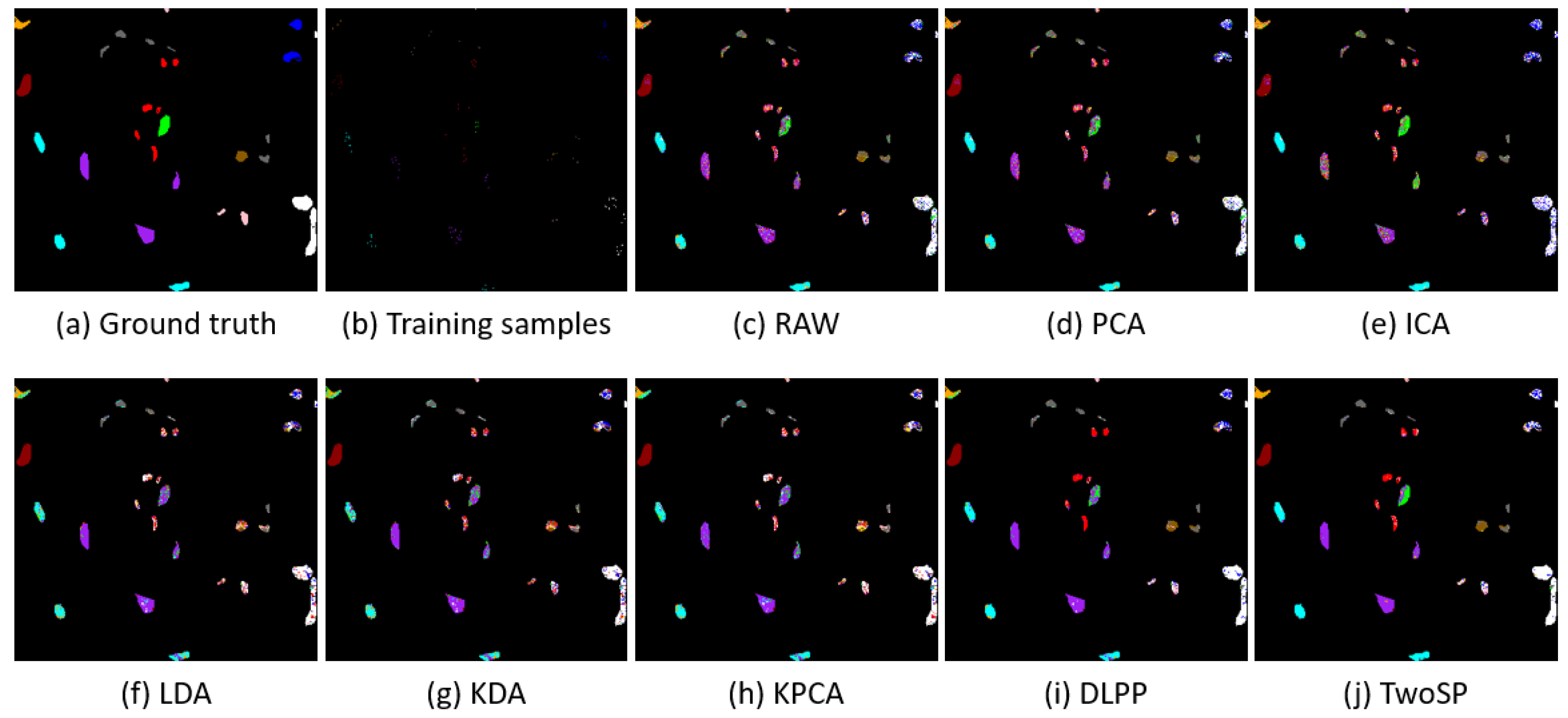
Furthermore, the classification maps of the aforementioned methods on Indian Pines and KSC datasets are visualized in Figure 1 and Figure 2. RAW, PCA, ICA, and KPCA have low classification performance because they cannot use the discrimination information in the subspace projection process. Although LDA and KDA use the discrimination information, they introduce all the within-class and between-class samples in the discriminant analysis, which is difficult to preserve the local manifold structure. From the subfigures (f) and (g) in Figure 1 and Figure 2, a clear classification map is shown for several classes. TwoSP, which enforces the discrimination information in a small neighborhood, shows better visualization quality than the others, since it not only preserves the global structure in the first-stage KPCA subspace projection, but also learns the local data relationship in the second-stage DLPP subspace projection. It also demonstrates that the utilization of discrimination information within a small neighborhood can largely improve the classification performance in the corresponding nonlinear feature space.

To further validate the effectiveness of the proposed method, we conducted an additional experiment by the effective cross validation method, i.e., the McNemar test [42].

Table 4. McNemar test of different methods on the Indian Pines and KSC datasets.

Methods	Indian Pines							KSC
	PCA	ICA	LDA	KDA	KPCA	DLPP	TwoSP	PCA	ICA	LDA	KDA	KPCA	DLPP	TwoSP
RAW	−0.3	20.8	−1.9	−1.3	20.2	−4.9	−18.7	0.9	26.6	−3.0	24.3	26.9	−1.3	−9.4
PCA	-	21.5	−1.7	−1.2	20.9	−4.7	−18.1	-	26.5	−3.1	24.2	26.8	−1.2	−9.5
ICA	-	-	−19.3	−19.1	−1.5	−22.1	−33.7	-	-	−24.5	−4.7	−1.0	−21.7	−25.4
LDA	-	-	-	0.7	18.6	−3.6	−15.5	-	-	-	21.9	24.3	5.5	−7.1
KDA	-	-	-	-	18.5	−3.9	−17.4	-	-	-	-	4.2	−18.8	−23.1
KPCA	-	-	-	-	-	−21.4	−33.2	-	-	-	-	-	−21.5	−25.1
DLPP	-	-	-	-	-	-	−12.8	-	-	-	-	-	-	−10.2

shows the results of the McNemar test for the proposed method and the baselines, where the methods on the vertical direction are the test methods, while those on the horizontal direction are the reference methods. When the value is greater than zero, it illustrates that the classification performance of the test method is better than that of the reference method; otherwise, the reference method has more advantages. Generally, the threshold of significance in the McNemar test is set to $0.05$. Furthermore, when the absolute value is larger than $1.96$, it indicts that the two methods have obvious differences. From Table 4, we can see that the TwoSP has the highest classification performance when compared with the existing approaches. In addition, the simplified version of our TwoSP, i.e., DLPP, also has good performance to some extent.

5.3. Discussion on Computational Cost

In this subsection, we only discuss the computational cost of the proposed method compared with state-of-the-art approaches. Considering the main steps in Algorithm 1, the proposed HSI classification method takes account of three parts: KPCA subspace projection, DLPP subspace projection, and classification.

Let $n_s$ and $n_t$ be the number of training and test samples, respectively. $n=n_s+n_t$. The computational complexity of first-stage subspace projection matrix, i.e., $\mathit{W}$, is $\mathcal{O}(n^3)$. Here, we can obtain the KPCA feature data ${\mathit{X}}_r$ with the dimensionality of r. k is denoted as the number of neighbors in the computation of adjacency matrix. The computational complexity of the second-stage subspace projection process is then $\mathcal{O}(rk{n}_s+r^3)$. After the two-stage subspace projection framework, the original HSI data is projected onto an optimal low-dimensional feature space with the dimensionality of m. For classification using NN classifier, each test sample is compared with all the training samples to find the nearest neighbor. Therefore, the computational complexity of classification is $\mathcal{O}(m{n}_t{n}_s)$.

Table 5. Computational time (s) of different methods on Indian Pines and KSC datasets.

Methods	Indian Pines				KSC
	T1	T2	T3	T4	T1	T2	T3	T4
RAW	-	1.67	35.48	2.84	-	0.42	20.63	2.88
PCA	0.68	0.70	21.48	0.92	0.28	0.19	12.81	0.67
ICA	11.69	0.66	21.36	3.19	5.41	0.17	8.44	0.52
LDA	0.20	0.62	17.64	0.63	0.08	0.18	7.58	0.31
KDA	1.05	0.69	19.42	0.80	0.35	0.16	7.64	0.30
KPCA	423.63	0.83	26.03	1.60	89.23	0.31	16.70	0.66
DLPP	0.61	0.67	18.48	0.53	0.17	0.22	10.20	0.41
TwoSP	428.25	0.68	21.28	0.83	89.38	0.19	12.00	0.41

shows the computational time (in terms of seconds) of the proposed method and the baselines, where T1 represents the computation of projection for different methods, and T2, T3, and T4 are the classification time obtained by NN, RF, and SVM classifiers, respectively. Since the first-stage projection of TwoSP needs to compute the kernel matrix (i.e., $\mathit{K}$) with all the training and test samples, T1 of TwoSP is larger than that of other methods. The T1s of KPCA and TwoSP are similar because they both involve in the computation of a large kernel matrix. KDA uses the discriminant information of a small portion of training samples, so the computation of its kernel matrix is small. RAW directly puts the original HSI data into the classification process, so its T1 is null. Among the T2, T3, and T4 of different methods, we can see that the RF classifier needs more time to classify all test samples. Considering classification performance and computational time simultaneously, we chose the NN classifier in the experiments.

5.4. Performance of Reduced Dimensionality

Each method is performed with different reduced dimensionality. To demonstrate the optimal reduced dimensionality for the corresponding method, the classification accuracy in terms of overall accuracy is obtained by the NN classifier when the dimensionality varies within $\{2,3,\cdots ,30\}$ on Indian Pines and KSC, respectively.

Figure 3 shows the curves of OA versus the reduced dimensionality on two different HSI datasets. The quantitative results are obtained with a random dataset partition. The proposed TwoSP method achieves the highest OA constantly. Especially, the OA value obtained by TwoSP exceeds that of the other methods to a large extent when the reduced dimensionality is more than 7. In Figure 3, the classification performance becomes stable when the dimensionality increases to a certain value. In most cases, the performance with low-dimensional projected data is better than the original high-dimensional data, which also validates that the dimensionality reduction does improve the classification accuracy.

5.5. Analysis of Classifier

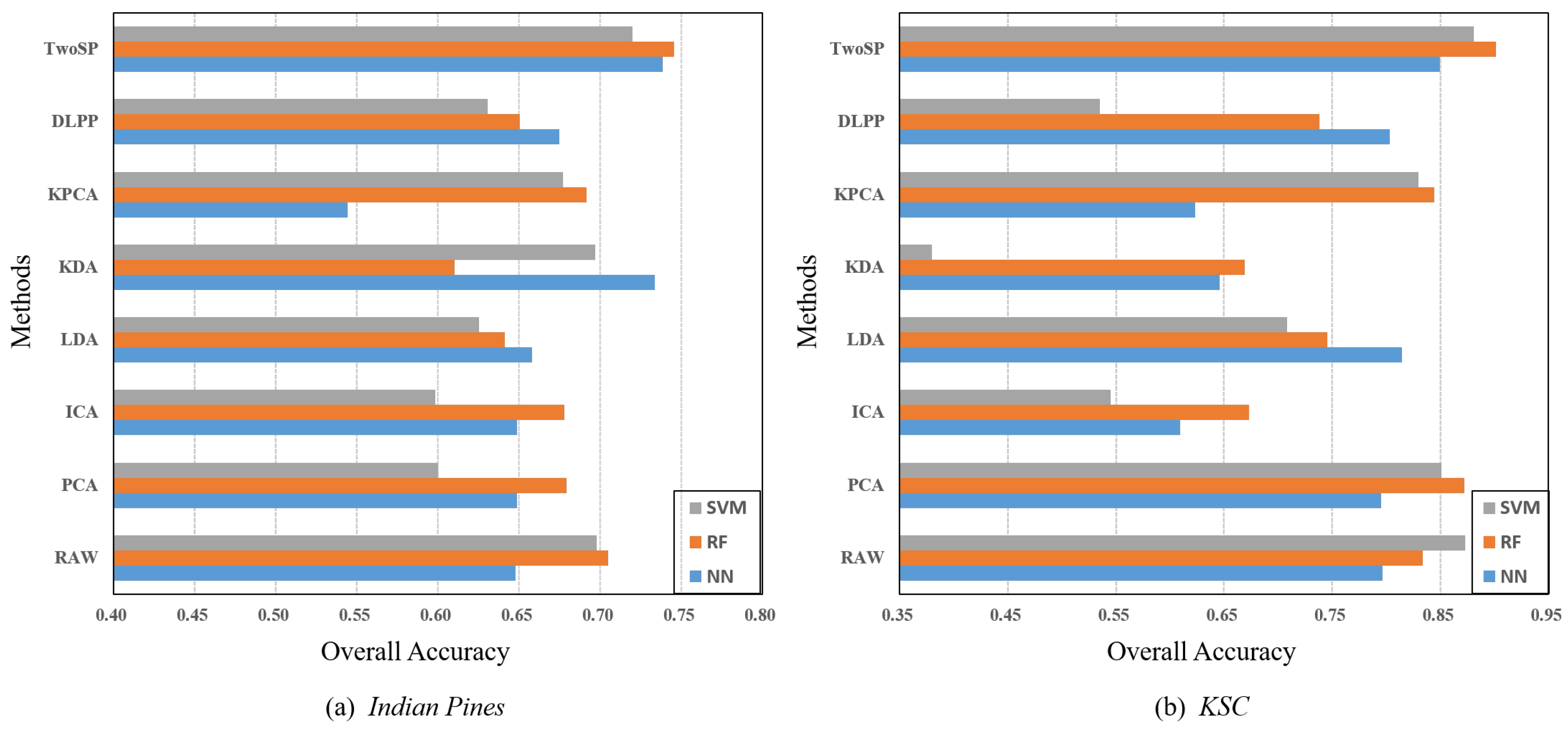
To evaluate the classification performance of each dimensionality reduction method with three different classifiers, i.e., NN, RF, and SVM, we randomly selected five different dataset partitions and then computed the average OA values. After the projected feature data was obtained by one of these dimensionality reduction methods, the classes of the test set were discriminated by the NN, RF, and SVM classifiers, respectively. Figure 4 shows the classification results vs. different classifiers on two HSI datasets.

In Figure 4a,b, the proposed TwoSP method presents the best classification performance for different classifiers when compared with the other dimensionality reduction methods, which also demonstrates that TwoSP has better robustness in different classifiers. For most cases on the Indian Pines dataset, the NN and RF classifiers generates better OAs than the SVM classifier. On the other hand, the RF classifier achieves better results on the KSC dataset, while the results with NN are superior to RF for LDA and DLPP. It also illustrates the classification accuracy of different classifiers on different datasets may have relatively large differences. To unify the utilization of the classification model, we applied the NN classifier to evaluate the classification performance of each class in Table 2 and Table 3.

5.6. Analysis of Parameters

In our proposed TwoSP method, there are three parameters set first, as shown in the input of Algorithm 1. Therefore, the first- and second-stage subspace projection dimensionality r and m and the number of neighbors k are studied experimentally. We randomly choose one of the training and test set partition and mainly take the Indian Pines dataset for instance. The objective values of the parameters are changed during the analysis process.

Figure 5a shows the overall accuracy results obtained by simultaneously varying the dimensionalities r and m. Since the first-stage subspace projection is designed to preserve the global structure of the original HSI data, the dimensionality of the second-stage subspace projection m should be smaller than r. From this subfigure, we can see that TwoSP is robust to r and m in a wide range. When r and m increase to a certain value, the classification performance in terms of OA is the best. Therefore, we select $r=45$ and $m=20$ for the Indian Pines dataset in the experiments. Figure 5b shows the different OA values vs. different number of neighbors in the second-stage subspace projection. TwoSP achieves the highest OA value when the number of neighbors $k=200$, which is chosen in this paper. Note that the neighbors are selected by comparing the kernel distances first. Only the within-class samples are used to compute the value of adjacency matrix, and zero otherwise. Therefore, in practice a small number of training samples are used to learn the local structure of the first-stage projected data.

6. Conclusions

In this paper, we proposed the TwoSP method on the basis of the preservation of global and local structures to learn the optimal low-dimensional feature space for HSI classification. TwoSP first applies the traditional KPCA method to address the nonlinear problem which often exists in the HSI data. However, the dimensionality of the first-stage subspace projection is not small enough. It needs to apply the second-stage subspace projection to the preceding projected features. TwoSP exploits the a priori knowledge of the training samples to construct an adjacency matrix for the within-class samples, which can enhance the discrimination information of projected features.

Compared with the state of the art, TwoSP is better able to learn the data manifold relationship in the desired feature space, which creates various valuable features for HSI classification. In addition, TwoSP strongly retains the local smoothness within a small neighborhood. Through the experiments on two real-world HSI datasets, i.e., Indian Pines and KSC, TwoSP provides better classification performance than the existing dimensionality reduction methods, which also validates the effectiveness of the proposed method.

Our future work will focus on how to extend the proposed method to train the optimal transformation matrix for each test sample quickly. It is desirable to improve the classification performance and increase the computation efficiency of the dimensionality reduction.

References

- Stein, D.W.J.; Beaven, S.G.; Hoff, L.E.; Winter, E.M.; Schaum, A.P.; Stocker, A.D. Anomaly detection from hyperspectral imagery. IEEE Signal Process. Mag. 2002, 19, 58–69. [Google Scholar] [CrossRef] [Green Version]
- Gevaert, C.M.; Suomalainen, J.; Tang, J.; Kooistra, L. Generation of Spectral-Temporal Response Surfaces by Combining Multispectral Satellite and Hyperspectral UAV Imagery for Precision Agriculture Applications. IEEE J. Sel. Top. Appl. Earth Obs. Remote Sens. 2015, 8, 3140–3146. [Google Scholar] [CrossRef]
- Luo, F.; Du, B.; Zhang, L.; Zhang, L.; Tao, D. Feature Learning Using Spatial-Spectral Hypergraph Discriminant Analysis for Hyperspectral Image. IEEE Trans. Cybern. 2018, PP, 1–14. [Google Scholar] [CrossRef] [PubMed]
- Liu, W.; Ma, X.; Zhou, Y.; Tao, D.; Cheng, J. p-Laplacian Regularization for Scene Recognition. IEEE Trans. Cybern. 2018, 1–14. [Google Scholar] [CrossRef] [PubMed]
- Wang, Q.; Liu, S.; Chanussot, J.; Li, X. Scene Classification with Recurrent Attention of VHR Remote Sensing Images. IEEE Trans. Geosci. Remote Sens. 2018, PP, 1–13. [Google Scholar] [CrossRef]
- Ma, X.; Liu, W.; Li, S.; Tao, D.; Zhou, Y. Hypergraph p-Laplacian Regularization for Remotely Sensed Image Recognition. IEEE Trans. Geosci. Remote Sens. 2018, 1–11. [Google Scholar] [CrossRef]
- Hughes, G. On the mean accuracy of statistical pattern recognizers. IEEE Trans. Inf. Theory 1968, 14, 55–63. [Google Scholar] [CrossRef]
- Mitra, P.; Murthy, C.A.; Pal, S.K. Unsupervised feature selection using feature similarity. IEEE Trans. Pattern Anal. Mach. Intell. 2002, 24, 301–312. [Google Scholar] [CrossRef] [Green Version]
- Wang, Q.; Lin, J.; Yuan, Y. Salient Band Selection for Hyperspectral Image Classification via Manifold Ranking. IEEE Trans. Neural Netw. Learn. Syst. 2016, 27, 1279–1289. [Google Scholar] [CrossRef] [PubMed]
- Liu, W.; Yang, X.; Tao, D.; Cheng, J.; Tang, Y. Multiview dimension reduction via Hessian multiset canonical correlations. Inf. Fusion 2018, 41, 119–128. [Google Scholar] [CrossRef]
- Wang, Q.; He, X.; Li, X. Locality and Structure Regularized Low Rank Representation for Hyperspectral Image Classification. IEEE Trans. Geosci. Remote Sens. 2018, PP, 1–13. [Google Scholar] [CrossRef]
- Zhang, L.; Zhang, L.; Tao, D.; Huang, X.; Du, B. Hyperspectral Remote Sensing Image Subpixel Target Detection Based on Supervised Metric Learning. IEEE Trans. Geosci. Remote Sens. 2014, 52, 4955–4965. [Google Scholar] [CrossRef]
- Luo, Y.; Wen, Y.; Tao, D.; Gui, J.; Xu, C. Large Margin Multi-Modal Multi-Task Feature Extraction for Image Classification. IEEE Trans. Image Process. 2016, 25, 414–427. [Google Scholar]
- Zhang, L.; Zhang, Q.; Du, B.; Huang, X.; Tang, Y.Y.; Tao, D. Simultaneous Spectral-Spatial Feature Selection and Extraction for Hyperspectral Images. IEEE Trans. Cybern. 2018, 48, 16–28. [Google Scholar] [CrossRef] [PubMed]
- Tao, D.; Tang, X.; Li, X. Which Components Are Important For Interactive Image Searching? IEEE Trans. Circuits Syst. Video Technol. 2008, 18, 3–11. [Google Scholar]
- Sun, W.; Tian, L.; Xu, Y.; Du, B.; Du, Q. A Randomized Subspace Learning Based Anomaly Detector for Hyperspectral Imagery. Remote Sens. 2018, 10, 417. [Google Scholar] [CrossRef]
- Luo, F.; Huang, H.; Duan, Y.; Liu, J.; Liao, Y. Local Geometric Structure Feature for Dimensionality Reduction of Hyperspectral Imagery. Remote Sens. 2017, 9, 790. [Google Scholar] [CrossRef]
- Li, X.; He, H.; Wang, R.; Tao, D. Single Image Superresolution via Directional Group Sparsity and Directional Features. IEEE Trans. Image Process. 2015, 24, 2874–2888. [Google Scholar] [CrossRef] [PubMed]
- Prasad, S.; Bruce, L.M. Limitations of Principal Components Analysis for Hyperspectral Target Recognition. IEEE Geosci. Remote Sens. Lett. 2008, 5, 625–629. [Google Scholar] [CrossRef]
- Wang, J.; Chang, C.I. Independent component analysis-based dimensionality reduction with applications in hyperspectral image analysis. IEEE Trans. Geosci. Remote Sens. 2006, 44, 1586–1600. [Google Scholar] [CrossRef] [Green Version]
- Wang, H.; Lu, X.; Hu, Z.; Zheng, W. Fisher Discriminant Analysis With L1-Norm. IEEE Trans. Cybern. 2014, 44, 828–842. [Google Scholar] [CrossRef] [PubMed]
- Wang, Z.; He, B. Locality perserving projections algorithm for hyperspectral image dimensionality reduction. In Proceedings of the 2011 19th International Conference on Geoinformatics, Shanghai, China, 24–26 June 2011; pp. 1–4. [Google Scholar]
- Bandos, T.V.; Bruzzone, L.; Camps-Valls, G. Classification of Hyperspectral Images With Regularized Linear Discriminant Analysis. IEEE Trans. Geosci. Remote Sens. 2009, 47, 862–873. [Google Scholar] [CrossRef] [Green Version]
- Wang, Q.; Meng, Z.; Li, X. Locality Adaptive Discriminant Analysis for Spectral-Spatial Classification of Hyperspectral Images. IEEE Geosci. Remote Sens. Lett. 2017, 14, 2077–2081. [Google Scholar] [CrossRef]
- Dong, Y.; Du, B.; Zhang, L.; Zhang, L. Dimensionality Reduction and Classification of Hyperspectral Images Using Ensemble Discriminative Local Metric Learning. IEEE Trans. Geosci. Remote Sens. 2017, 55, 2509–2524. [Google Scholar] [CrossRef]
- Fauvel, M.; Chanussot, J.; Benediktsson, J.A. Kernel Principal Component Analysis for the Classification of Hyperspectral Remote Sensing Data over Urban Areas. EURASIP J. Adv. Signal Process. 2009, 2009, 783194. [Google Scholar] [CrossRef]
- Mei, F.; Zhao, C.; Wang, L.; Huo, H. Anomaly Detection in Hyperspectral Imagery Based on Kernel ICA Feature Extraction. In Proceedings of the 2008 Second International Symposium on Intelligent Information Technology Application, Shanghai, China, 20–22 December 2008; Volume 1, pp. 869–873. [Google Scholar]
- Baudat, G.; Anouar, F. Generalized Discriminant Analysis Using a Kernel Approach. Neural Comput. 2000, 12, 2385–2404. [Google Scholar] [CrossRef] [PubMed] [Green Version]
- Li, X.; He, H.; Yin, Z.; Chen, F.; Cheng, J. Single image super-resolution via subspace projection and neighbor embedding. Neurocomputing 2014, 139, 310–320. [Google Scholar] [CrossRef]
- Feng, J.; Liu, L.; Cao, X.; Jiao, L.; Sun, T.; Zhang, X. Marginal Stacked Autoencoder With Adaptively-Spatial Regularization for Hyperspectral Image Classification. IEEE J. Sel. Top. Appl. Earth Obs. Remote Sens. 2018, 11, 3297–3311. [Google Scholar] [CrossRef]
- Borges, J.S.; Bioucas-Dias, J.M.; Marcal, A.R.S. Bayesian Hyperspectral Image Segmentation With Discriminative Class Learning. IEEE Trans. Geosci. Remote Sens. 2011, 49, 2151–2164. [Google Scholar] [CrossRef] [Green Version]
- Fauvel, M.; Dechesne, C.; Zullo, A.; Ferraty, F. Fast Forward Feature Selection of Hyperspectral Images for Classification With Gaussian Mixture Models. IEEE J. Sel. Top. Appl. Earth Obs. Remote Sens. 2015, 8, 2824–2831. [Google Scholar] [CrossRef]
- Cariou, C.; Chehdi, K. A new k-nearest neighbor density-based clustering method and its application to hyperspectral images. In Proceedings of the 2016 IEEE International Geoscience and Remote Sensing Symposium (IGARSS), Beijing, China, 10–15 July 2016; pp. 6161–6164. [Google Scholar]
- Li, J.; Bioucas-Dias, J.M.; Plaza, A. Semisupervised Hyperspectral Image Segmentation Using Multinomial Logistic Regression With Active Learning. IEEE Trans. Geosci. Remote Sens. 2010, 48, 4085–4098. [Google Scholar] [CrossRef]
- Xu, Y. Maximum Margin of Twin Spheres Support Vector Machine for Imbalanced Data Classification. IEEE Trans. Cybern. 2017, 47, 1540–1550. [Google Scholar] [CrossRef] [PubMed]
- Pullanagari, R.R.; Kereszturi, G.; Yule, I. Integrating Airborne Hyperspectral, Topographic, and Soil Data for Estimating Pasture Quality Using Recursive Feature Elimination with Random Forest Regression. Remote Sens. 2018, 10, 1117. [Google Scholar] [CrossRef]
- De Bie, T.; Cristianini, N. Kernel Methods for Exploratory Pattern Analysis: A Demonstration on Text Data. In Structural, Syntactic, and Statistical Pattern Recognition; Springer: Berlin/Heidelberg, Germany, 2004; pp. 16–29. [Google Scholar]
- Li, X.; He, H.; Yin, Z.; Chen, F.; Cheng, J. KPLS-based image super-resolution using clustering and weighted boosting. Neurocomputing 2015, 149, 940–948. [Google Scholar] [CrossRef]
- Chen, M.; Wang, Q.; Li, X. Discriminant Analysis with Graph Learning for Hyperspectral Image Classification. Remote Sens. 2018, 10, 836. [Google Scholar] [CrossRef]
- Hyperspectral Remote Sensing Scenes. Available online: http://www.ehu.eus/ccwintco/index.php?title=Hyperspectral_Remote_Sensing_Scenes (accessed on 31 July 2018).
- Chang, C.C.; Lin, C.J. LIBSVM: A library for support vector machines. ACM Trans. Intell. Syst. Technol. 2011, 2, 27:1–27:27. Available online: http://www.csie.ntu.edu.tw/~cjlin/libsvm (accessed on 15 July 2018). [CrossRef]
- Eyden, R.J.V.; Wit, P.W.C.D.; Arron, J.C. Predicting company failure-a comparison between neural networks and established statistical techniques by applying the McNemar test. In Proceedings of the Conference on Computational Intelligence for Financial Engineering (CIFEr), New York, NY, USA, 9–11 April 1995; pp. 91–96. [Google Scholar]
Figure 1.
Classification maps for the Indian Pines dataset with different dimensionality reduction algorithms using NN classifier. (a) The ground truth of the classes. (b) Randomly selected training samples. (c) Result obtained by using RAW features. (d) PCA. (e) ICA. (f) LDA. (h) KDA. (g) KPCA. (i) the proposed DLPP. (j) The proposed TwoSP.
Figure 2.
Classification maps (cropped to a size of 290 × 310) for the KSC dataset with different dimensionality reduction algorithms using NN classifier. (a) The ground truth of the classes. (b) Randomly selected training samples. (c) Result obtained by using RAW features. (d) PCA. (e) ICA. (f) LDA. (h) KDA. (g) KPCA. (i) The proposed DLPP. (j) The proposed TwoSP.
Figure 3.
Overall Accuracy (OA) obtained by the NN classifier versus the reduced dimensionality of various different methods on two real-world HSI datasets, i.e., (a) Indian Pines and (b) KSC.
Figure 4.
Classification Results in terms of Overall Accuracy (OA) of each dimensionality reduction method with different classifiers on (a) Indian Pines and (b) KSC.
Figure 5.
Parameter analysis of (a) OAs with simultaneously varying the first-stage subspace projection dimensionality r and the second-stage subspace projection dimensionality m on Indian Pines, and (b) OAs with varying the number of neighbors k in the computation of adjacency matrix.