Bias Removal for Goldstein Filtering Power Using a Second Kind Statistical Coherence Estimator

Abstract

The adaptive Goldstein filter driven by InSAR coherence is one of the most famous frequency domain-based filters and has been widely used to improve the quality of InSAR measurement with different noise features. However, the filtering power is biased to varying degrees due to the biased coherence estimator and empirical modelling of the filtering power under a given coherence level. This leads to under- or over-estimation of phase noise over the entire dataset. Here, the authors present a method to correct filtering power on the basis of the second kind statistical coherence estimator. In contrast with regular statistics, the new estimator has smaller bias and variance values, and therefore provides more accurate coherence observations. In addition, a piece-wise function model determined from the Monte Carlo simulation is used to compensate for the nonlinear relationship between the filtering parameter and coherence. This method was tested on both synthetic and real data sets and the results were compared against those derived from other state-of-the-art filters. The better performance of the new filter for edge preservation and residue reduction demonstrates the value of this method.

1. Introduction

Synthetic aperture radar interferometry (InSAR) has developed rapidly in the last three decades. Because of its accuracy, convenience, and efficiency, InSAR is an effective tool for surface deformation monitoring [1], forest management and classification [2,3], and ocean currents and earthquake inversion [4,5]. Successful applications of this technique rely on the quality of the interferogram. However, SAR instruments suffer from both temporal and spatial decorrelation, leading to stochastic phase noises with different spatial features in InSAR measurements [6,7]. The general consensus among previous studies is that phase noise likely causes error propagation in data processing (e.g., phase unwrapping) and increases the uncertainty of the final InSAR products [8]. It is therefore imperative to provide effective filtering methods to enhance the quality of the interferogram and simultaneously preserve spatial information.

In recent years, many studies have tried to resolve the problem from spatial and frequency viewpoints. The Goldstein filter has proven to be a feasible method to improve the tradeoff between estimation accuracy and computational efficiency [7]. It smoothens the Fourier spectrum of the interferogram by using the strong anti-noise capacity available in the frequency domain. Although this approach is promising, it was developed for geophysical applications that span large geographic regions. Therefore, the fringe pattern and spatial information cannot be preserved in detail in the interferogram, leading to blurred image features and loss of the phase signal.

In order to identify higher resolution surface changes, variants to overcome the shortcoming of classical Goldstein filtering have been developed based on the quality maps of interferometric signals [9,10,11,12]. The key principle behind this is that strong noise areas are filtered more than low noise areas. The quality maps include coherence, theoretical phase standard deviation, the signal-to-noise ratio (SNR), and pseudo-correlation [9,10,13]. A common limitation of these methods is that statistical estimators of these quality maps are usually highly biased and therefore under-estimate the phase noise in the real word. Although some of them mitigate the bias by modeling the bias with empirical functions, most of the models are determined using subjective criteria. To compensate for the impact of biased estimation, several methods also consider iterative filtering, especially over fast decorrelation areas [12,13,14]. However, this behavior will likely cause artifactual fringe patterns because pure noise will contribute to the Fourier spectrum and filtering will confuse noise for fringes.

The primary objective of this paper was to develop, test, and validate a new method for InSAR interferogram filtering. This method resolves the issues mentioned above by accurately estimating the Goldstein filtering power. Specifically, (1) the weighted coherence estimator based on a second kind statistic is developed to calculate sample coherence. In contrast with regular statistics used in previous studies, this estimator has smaller bias and variance values, and can therefore infer better noise information for the interferogram; (2) a piece-wise function is established to quantify the filtering power using the Monte Carlo simulation. This model allows for heavy filtering over strong noise areas and preserves phase signals in areas with low noise. In the following sections, the authors outline the definition, describe the methods and results, and conclude with a discussion of lessons learned from this research.

2. Methodology

2.1. Adaptive Goldstein Filtering

Goldstein and Werner first proposed an adaptive radar interferogram filter and defined it as the multiplication of the Fourier spectrum $Z(u,v)$ of the interferogram patch by the smoothed modulus $S\left\{\left|Z(u,v)\right|\right\}$ raised to the power of an exponent $\alpha$:

$$H\left(u,v\right)=S{\left\{\left|Z\left(u,v\right)\right|\right\}}^{\alpha }\cdot Z\left(u,v\right),$$

(1)

where $H(u,v)$ denotes the filter response; $S\{\cdot \}$ denotes the smoothing operator; and $u$ and $v$ are spatial frequencies in each interferogram patch (e.g., $32\times 32$ window). The filtering power $\alpha$ is used to control the smoothness of filtering, which increases with larger $\alpha$ values. According to the definition in [7], $\alpha$ ranges from 0 to 1.

Each interferogram patch has different noise features. The use of a uniform value of $\alpha$ will under- or over-estimate the degree of noise, leading to significant changes to the structure of the interferogram. Therefore, adaptive behavior can be used to change $\alpha$ according to the quality of the interferogram [9]. For example, $\alpha$ can be defined as a linear model:

$$\alpha =1-\gamma ,$$

(2)

where parameter $\gamma$ is used to evaluate the phase noise and usually measured by InSAR coherence [15,16]. A higher value of $\gamma$ implies a lower noise degree and vice versa. $\gamma =1$ denotes a noise-free signal where the filter power $\alpha$ becomes zero and no filtering occurs.

2.2. Coherence Estimation Based on the Second Kind Statistic

2.2.1. Definition of the Coherence Estimator

One of the difficulties with Equation (2) is the fact that the estimator of coherence parameter $\gamma$ is highly biased. This limitation further under-estimates the value of $\alpha$, leading to under-filtering over low coherence regions. Therefore, it is necessary to obtain an accurate coherence estimation before filtering. The coherence estimator $\widehat{\gamma }$ is defined as:

$$\widehat{\gamma }=\frac{\left|{\displaystyle \sum _{i=1}^{n}w(i)z_1(i)z_2^{\ast }(i)}\right|}{\sqrt{{\displaystyle \sum _{i=1}^{n}w(i){\left|z_1(i)\right|}^2}{\displaystyle \sum _{i=1}^{n}w(i){\left|z_2(i)\right|}^2}}},$$

(3)

where $z_1$ and $z_2$ are single complex images (SLC) used for interferogram formalization and $n$ is the sample number in each estimate window. When weight $w=1$, the equation converts to the conventional coherence estimator defined in [15]. The effect of weight is to reduce the heterogeneity of neighboring pixels that need to be averaged. Therefore, according to the theory of WML estimation investigated in [17], $\widehat{\gamma }$ is a weighted maximum likelihood (WML) estimator.

2.2.2. Weight Determination Weight

The study takes advantage of the similarity between the reference pixel and its neighbors to determine the weight for Equation (3). The similarity is designed from the two-sample Anderson-Darling test statistic by [18,19]:

$$AD=\frac{ab}{N}{\displaystyle \underset{-\infty }{\overset{+\infty }{\int }}\frac{{\left(F_a(x)-G_b(x)\right)}^2}{H_N(x)\left(1-H_N(x)\right)}}d{H}_N(x),$$

(4)

where $F_a(x)$, $G_b(x)$, and $H_N(x)$ with $N=a+b$ are the empirical distribution functions (EDF) of a—samples, b—samples, and combined samples, respectively, and $H_N(x)=(a{F}_a(x)+b{G}_b(x))/N$. In this case, replacing a—samples and b—samples with $m$ pixels in a patch centered at the reference pixel ${\mathsf{\Theta }}_{ref}$ and a neighbor ${\mathsf{\Theta }}_{neig}$, respectively, to get $a=b=m$ and $N=2m$, and the test statistic, can be rewritten as:

$$AD=\frac{m}{2}{\displaystyle \sum \frac{{\left(F_{{\mathsf{\Theta }}_{ref}}(x)-G_{{\mathsf{\Theta }}_{neig}}(x)\right)}^2}{H_{{\mathsf{\Theta }}_{ref}\cup {\mathsf{\Theta }}_{neig}}(x)\left(1-H_{{\mathsf{\Theta }}_{ref}\cup {\mathsf{\Theta }}_{neig}}(x)\right)}},$$

(5)

where $F_{{\mathsf{\Theta }}_{ref}}(x)$ and $G_{{\mathsf{\Theta }}_{neig}}(x)$ denote the EDF of reference and neighboring pixels, respectively, and are estimated from $m$ samples in each patch, while $H_{{\mathsf{\Theta }}_{ref}\cup {\mathsf{\Theta }}_{neig}}(x)$ is the EDF of the combined samples in both patches.

The Anderson-Darling (AD) test is a non-parametric test and a measurement of distance between two distributions [19]. Looking at the numerator in Equation (5), the AD distance places more weight on observations towards the tails of the distribution. Thus, it is a better measure than its competitors, such as the Cramér–von Mises and Kolmogorov–Smirnov statistics. Given the fact that AD is proportional to the difference between two distributions, it can be used to measure the homogeneity between two pixels by using their samples in patches.

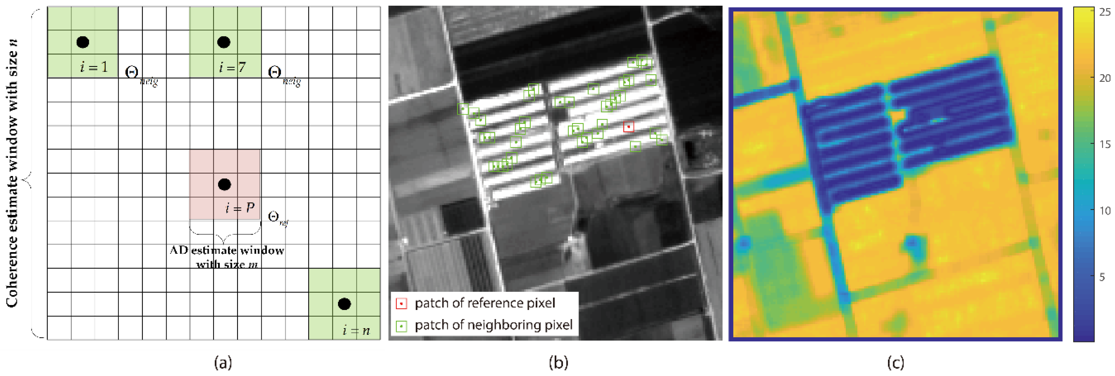
Let AD(i) be the value of the ith pixel in the coherence estimate window centered at a reference pixel P. Each AD(i) corresponding to P is estimated by sliding a window of size $m$ (Figure 1a). This procedure is repeated until the estimation for the nth pixel is finished. Throughout this paper, a $5\times 5$ window size is used to estimate AD values and $m=25$. It is always less than that used to calculate coherence in Equation (3) and therefore $n>m$. Figure 1b presents footprints of similarity patches ${\mathsf{\Theta }}_{neig}$ (green) passed by the Anderson-Darling test under a significance level of $\alpha =0.01$, and all AD values corresponding to the reference pixel P have been shown in Figure 1c. Visually, pixels sharing similar backscattering features with the reference pixel (Figure 1b) have smaller AD values, while pixels with other textures have larger AD values.

The weight by the reciprocal of the test statistic is defined as:

$$w(i)=\frac{1/AD(i)}{{\displaystyle \sum _{i=1}^n\left(1/AD(i)\right)}},$$

(6)

It is worth pointing out that for patch ${\mathsf{\Theta }}_{ref}={\mathsf{\Theta }}_{neig}$, $AD(P)=0$, and it makes no sense to apply weighting in coherence estimation. Instead, $AD(P)=0.1$ is set according to 1000 simulated scenes with different textures. The method used to determine the optimal weight as 0.1 for the reference pixel is the same as in [20], where overall errors between true and estimated values from all possible weight values were explored for each scene and the weight with minimum error was selected.

From a statistical viewpoint, there is no significance in estimating coherence by means of samples from different populations. Thus, the effect of weighting is to reduce spatial sample heterogeneity and to assign larger weights to those pixels that follow the same distribution as the reference pixel. Since SAR backscattering is usually used as a proxy for phase stability, the AD test is applied to intensity SAR [21]. From the image processing viewpoint, same surface targets generally share similar backscattering properties, showing the same textures in SAR images. The selection of homogeneous pixels with respect to the reference pixel can preserve the image resolution and mitigate the edge-smearing phenomenon [22]. However, because isolated targets may increase the variance of the estimated coherence image, the weighting strategy was developed to reduce the variance.

2.2.3. Bias Removal Using Second Kind Statistic Estimator

Nicolas and Anfinsen (2002) introduced second kind statistics based on the characteristic functions that substitute the Fourier transformation with the Mellin transformation [23]. It has been demonstrated that the second kind variances are considerably lower than regular variances for probability density functions defined on $R^{+}$ and slightly higher than the Cramer-Rao bound [23]. By deriving the second kind first characteristic function, the Mellin transformation allows the user to define the following second kind moments [23,24],

$${\tilde{m}}_v={{\displaystyle {\int }_0^{+\infty }\left(\ln \left(u\right)\right)}}^v{p}_x\left(u\right)du,$$

(7)

where ${\tilde{m}}_v$ denotes the second kind moment of the order $v$ and $p_x(u)$ is the probability density function (PDF) of a specified random variable. Given PDF of sample coherence $\widehat{\gamma }$ [24],

$$p(\widehat{\gamma }|\gamma ,n)=2\widehat{\gamma }\left(n-1\right){\left(1-{\gamma }^2\right)}^n{\left(1-{\widehat{\gamma }}^2\right)}^{\left(n-2\right)}{}_{2}F_1\left(n,n;1;{\widehat{\gamma }}^2{\gamma }^2\right),$$

(8)

where $\gamma$ and $n$ are the true coherence and the number of samples used to estimate sample coherence $\widehat{\gamma }$ in Equation (3), respectively, and ${}_{2}F_1(\cdot )$ denotes the ordinary hypergeometric function. Let $v=1$ and one can deduce the second kind mean by:

$${\tilde{m}}_1={\displaystyle {\int }_0^1\ln \left(\widehat{\gamma }\right)}p\left(\widehat{\gamma }|\gamma ,n\right)d\widehat{\gamma },$$

(9)

and the equivalent expectation of second kind mean is then defined as:

$$E\left(\widehat{\gamma }\right)=e^{{\tilde{m}}_1},$$

(10)

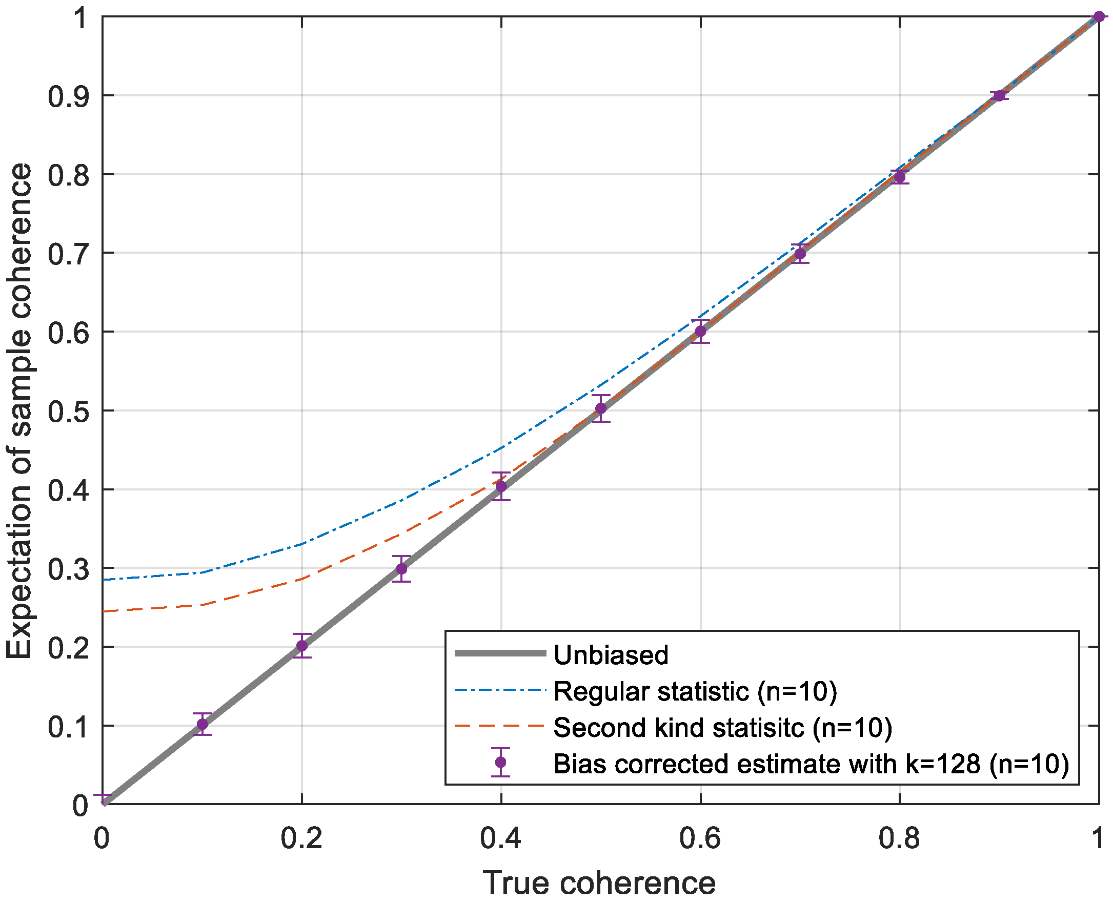
Figure 2 represents the expectation of sample coherence as a function of true coherence, in which the dashed line indicates the bias of the second kind statistic coherence estimator and is calculated by combining Equations (8)–(10) under each true coherence $\gamma$, while the dash-dotted line denotes the bias of the regular coherence estimator and is calculated by Equation (6) in [16]. It can be seen that the sample coherence from the regular statistic is more biased than from the second kind statistic in Equation (10), especially over low coherence regions. However, the bias of the second kind estimator cannot be completely removed by inverting (10) because the analytical expressions for Equation (9) are not existent. If a sufficiently large number k of independent sample coherence $\widehat{\gamma }$ are averaged:

$$\overline{\widehat{\gamma }}=\frac{{\displaystyle \sum _{i=1}^k\ln \left(\widehat{\gamma }(i)\right)}}{k},$$

(11)

the second kind mean estimate $\overline{\widehat{\gamma }}$ tends to be distributed normally around ${\tilde{m}}_1$, with the variance var($\widehat{\gamma }$)/k. Therefore, a bias corrected estimate can be obtained at $E\left(\widehat{\gamma }\right)\approx e^{\overline{\widehat{\gamma }}}$,

$$\tilde{\gamma }:Fun{c}^{-1}\left(E\left(\widehat{\gamma }\right)\approx e^{\overline{\widehat{\gamma }}}\right),$$

(12)

$E\left(\widehat{\gamma }\right)$ can be substituted with its ML estimate $e^{\overline{\widehat{\gamma }}}$ in Equation (10), which is inverted according to Equation (12) to deduce an unbiased coherence estimate $\tilde{\gamma }$. Tables of inversion are first calculated using Equations (8)–(10) to reduce the computational burden. Similar tables were obtained in [16] using simulations in the open source SHPS-InSAR toolbox that is available at http://mijiang.org.cn/index.php/software/. In reality, the sample mean in Equation (11) is calculated from the area in the coherence map covered by an effective patch in Goldstein filtering (patch minus the overlapping area: $32\times 32$ window size with 28 overlapping pixels). Thus, $k=128$ so that $\overline{\widehat{\gamma }}$ approximates to $E\left(\widehat{\gamma }\right)$. The performance of the unbiased estimate at $k=128$ with its standard deviation is shown in purple in Figure 2.

2.3. Modeling Filtering Power Using Unbiased Coherence

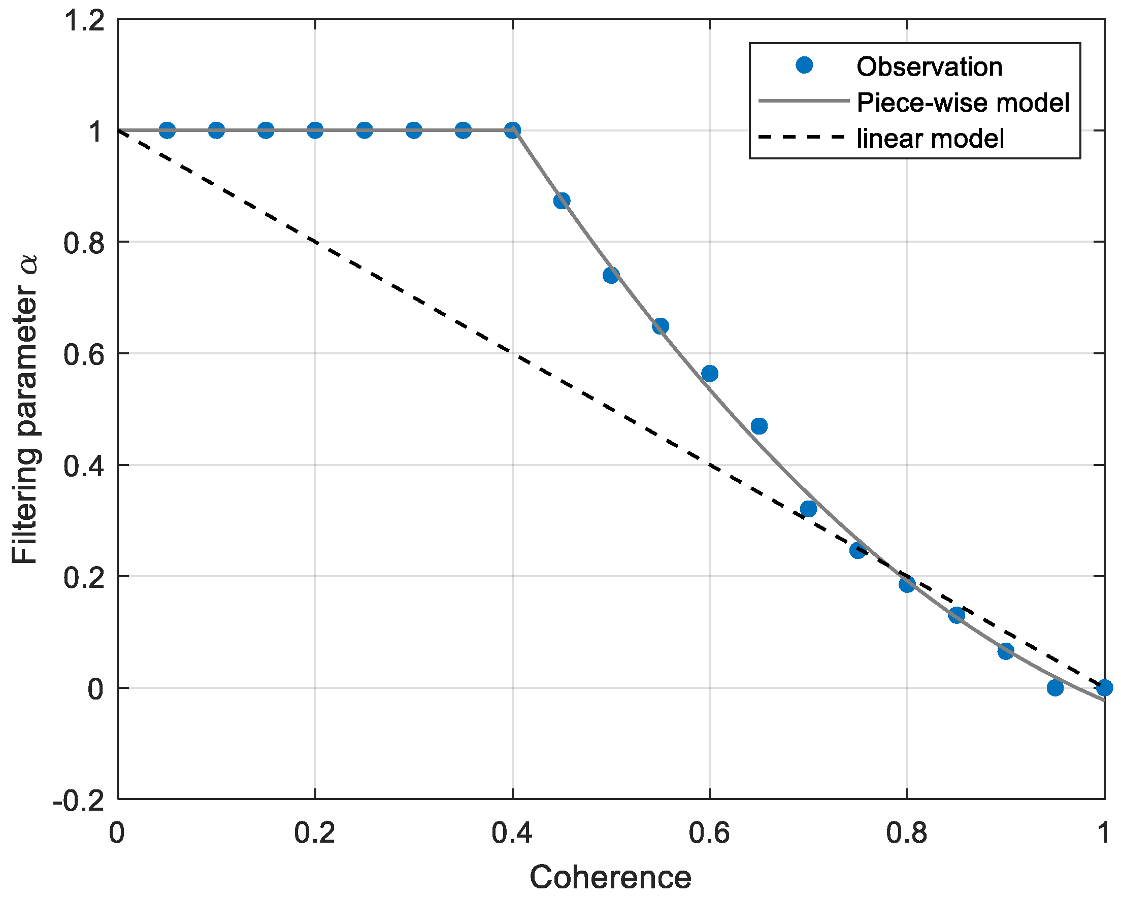
Unbiased coherence can quantify the quality of the interferogram more accurately and the mitigation of heterogeneity in the coherence map further increases the spatial resolution of filtering. This ensures that the coherence map can guide Goldstein filtering correctly. However, the filtering power over noise areas is still biased due to the unknown relationship between the filtering parameter used and the coherence magnitude. Therefore, the impact of filtering on different fringe patterns is investigated under each coherence level and the optimal filtering power is determined by minimizing the difference between the noise-free and filtered interferograms based on the Monte Carlo simulation. Specifically, the noise-free interferogram was first simulated using the universal multifractal technique with random multifractal parameter settings [25]. The noise interferogram was then generated by adding phase noise with specified phase standard deviation, which is a function of coherence [26]. Given 1000 noise interferograms with different patterns under a coherence level $\gamma \in \{0,0.1,\dots ,1\}$, each of them was filtered by Goldstein filtering with discrete parameter ($\alpha$) values from 0 to 1 and evaluated against the noise-free image using root mean square error (RMSE). The optimal filtering power $\alpha$ was finally determined by maximizing the number of times that $\alpha$ corresponding to minimum RMSE in each of 1000 trials was considered optimal.

Figure 3 presents the coherence level versus optimal filtering power. Compared with the empirical model (dashed line) of the Baran filter presented in previous studies [9], non-linear characteristics can be clearly observed in this case. This explains one of the reasons why under-filtering generally occurs in the Baran filter. To correct this bias, the piece-wise function model (solid line) was deployed to fit the trajectory by iterative reweighted least squares and can be expressed as:

$$\alpha =\{\begin{array}{ll}1,& \tilde{\gamma }\le 0.4\\ 1.61{\tilde{\gamma }}^2-3.96\tilde{\gamma }+2.33,& \tilde{\gamma }>0.4\end{array},$$

(13)

2.4. Filter Development

The modification of bias correction for filtering power leads to a newly developed Goldstein filter, which can be presented schematically as follows:

(1)

For each image pixel P, a coherence estimate window of size n is defined. The similarity between P and its neighbors is compared individually on an average intensity SAR image with patch size m (Figure 1a), and the weight of the coherence estimate window is confirmed using Equation (6). The sample coherence for pixel P is then estimated using Equation (3).

(2)

The procedure is repeated until the sample coherence of the last pixel in the whole image is estimated and coherence map is generated.

(3)

Goldstein filtering is performed on the interferogram in which the coherence sample with size k in each filtering patch is first averaged to obtain $\overline{\widehat{\gamma }}$ using Equation (11), and is further corrected to unbiased coherence $\tilde{\gamma }$ according to Equation (12).

(4)

The filtering power is adjusted according to Equation (13) and Goldstein filtering is performed on such patches.

(5)

Steps (3) and (4) are repeated until the whole interferogram has been filtered.

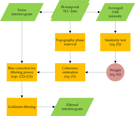
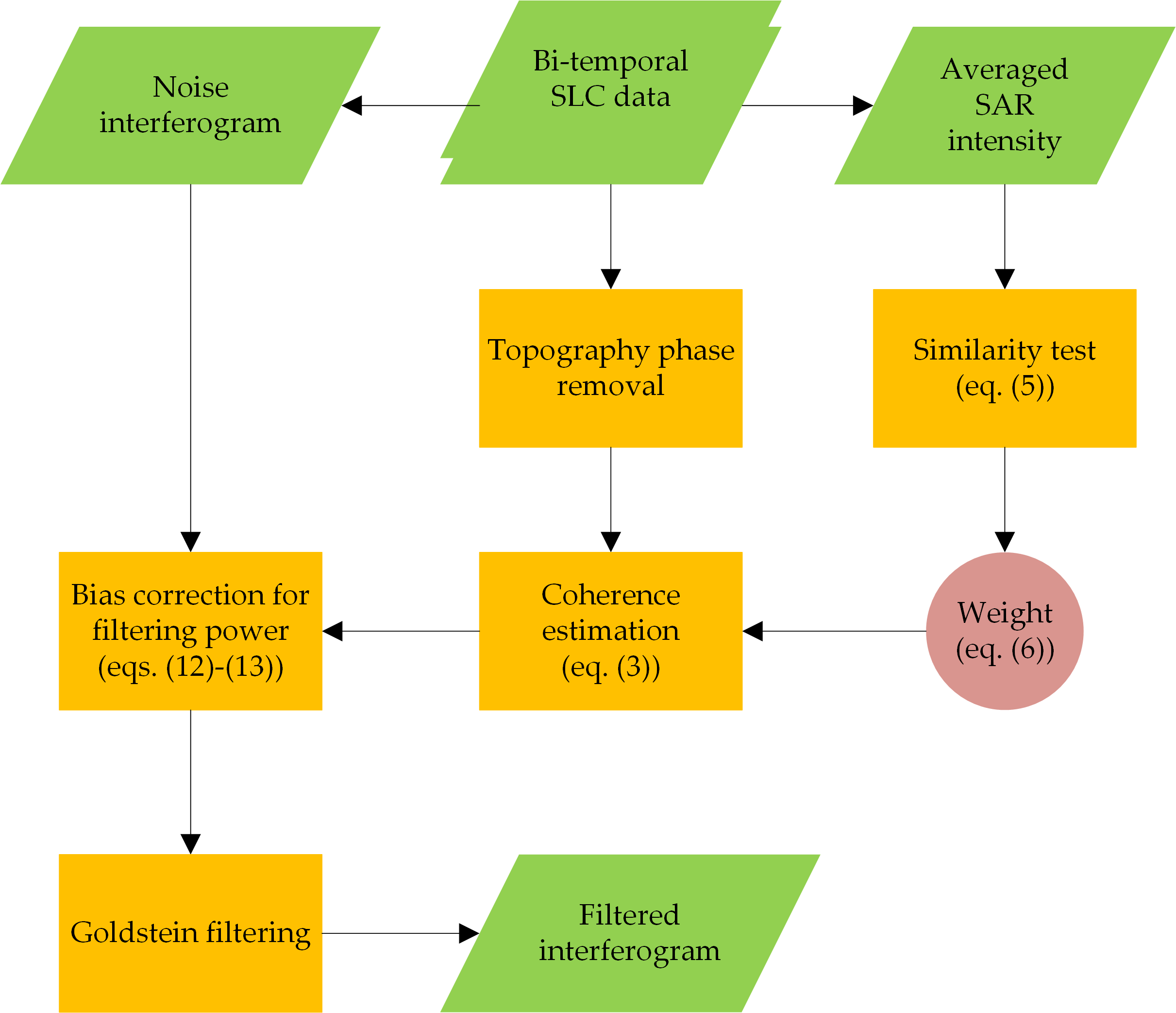
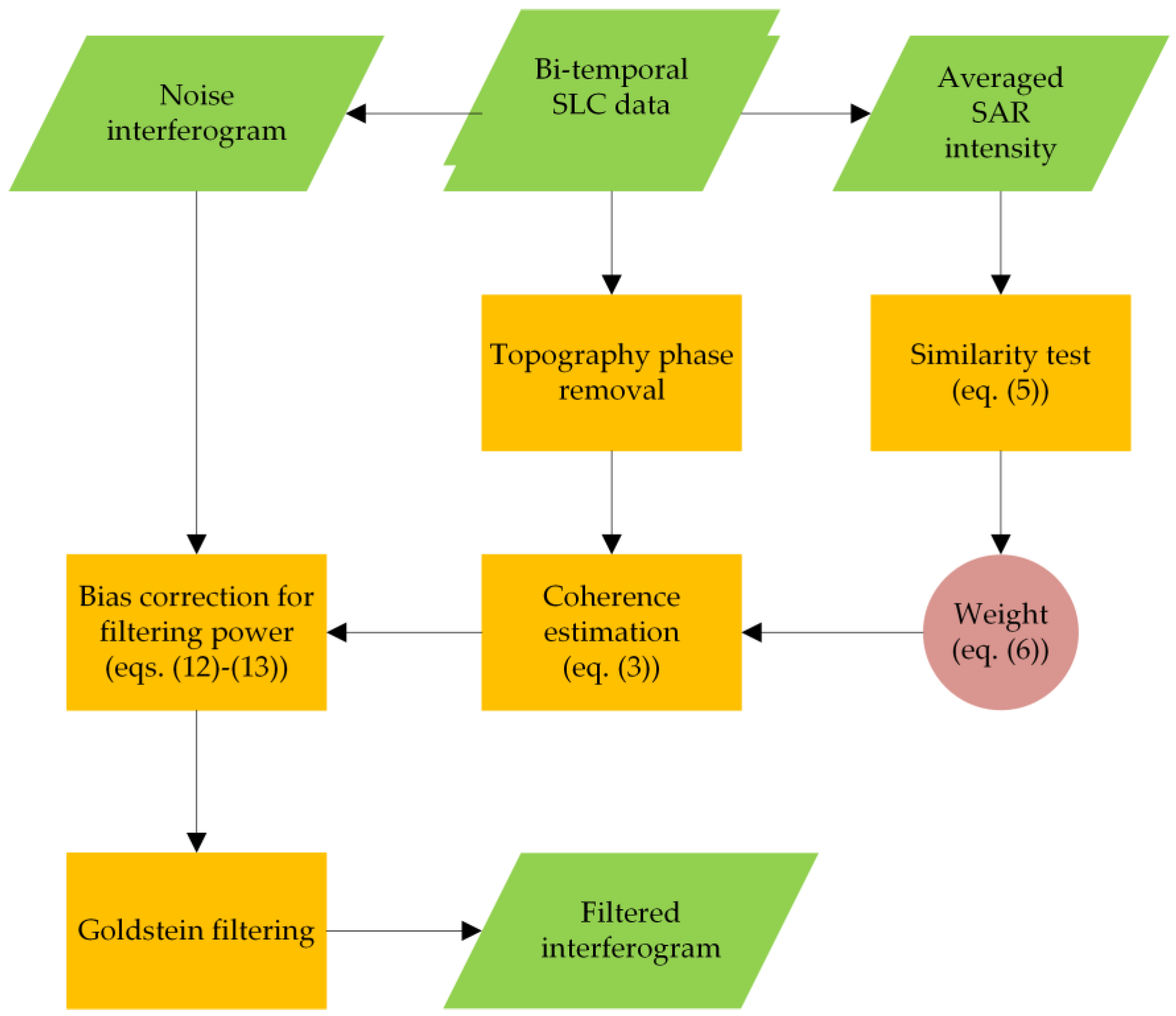
For this paper, the coherence window size in step (1) is set to $15\times 15(n=225)$ and the similarity patch is $5\times 5(m=25)$. In steps (3) and (4), the filtering window is set to be $32\times 32$ with the overlaps between windows set at 28 pixels, leading to the averaged coherence sample number k = 128. The flowchart of the proposed algorithm is shown in Figure 4.

3. Results and Discussion

3.1. Synthetic Data

To investigate the effectiveness of the newly developed filter, the authors compared the results from both synthetic and real data against those of state-of-the-art filters, including the Baran filter [9], the adaptive Goldstein filter derived from unbiased coherence under regular statistics (AGFC) [11], and iterative pseudo-correlation (AGFP) [13]. Without loss of generality, the classical window size $7\times 7$ was used for AGFC and AGFP to estimate map quality.

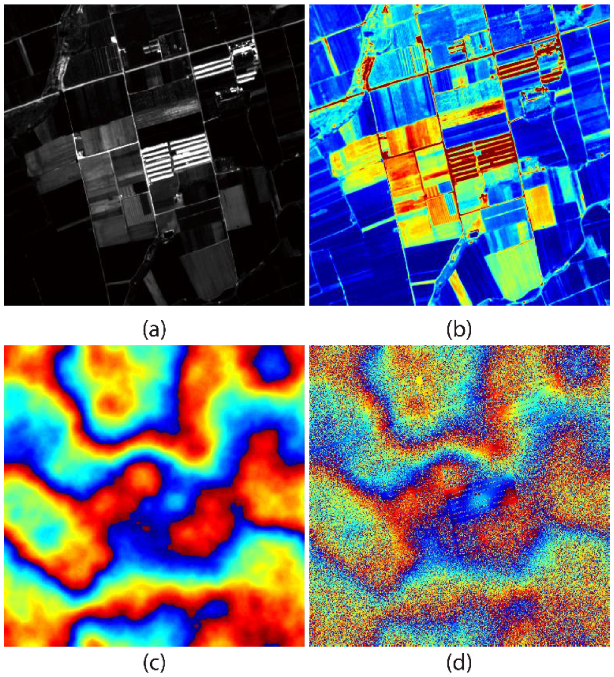
The simulation starts from bi-temporal SLC imagery $z_1$ and $z_2$, and proceeds as follows: (1) generate image patterns with different spatial distributions. Given the independence between intensity and phase pattern, a panchromatic Gaofen-2 image with $400\times 400$ pixels over the Shandong area was used as a noise-free SAR intensity images ($I$) (Figure 5a), and the coherence map ($\gamma$) was simulated by normalizing the Gaofen-2 image in the interval [0,1] (Figure 5b). The noise-free interferometric phase $\varphi$ was simulated using the universal multifractal technique (Figure 5c); (2) generate noise image according to a covariance matrix:

$$\left(\begin{array}{l}{z}_1\\ z_2\end{array}\right)={\left(\begin{array}{cc}I& I\gamma e^{-j\varphi }\\ I\gamma e^{j\varphi }& I\end{array}\right)}^{1/2}\left(\begin{array}{l}{x}_1\\ x_2\end{array}\right),$$

(14)

where $x_1$ and $x_2$ are independent complex Gaussian random variables with zero mean and unit variance. The corresponding noise interferogram after the conjugation operator $z_1{z}_2^{\ast }$ is shown in Figure 5d.

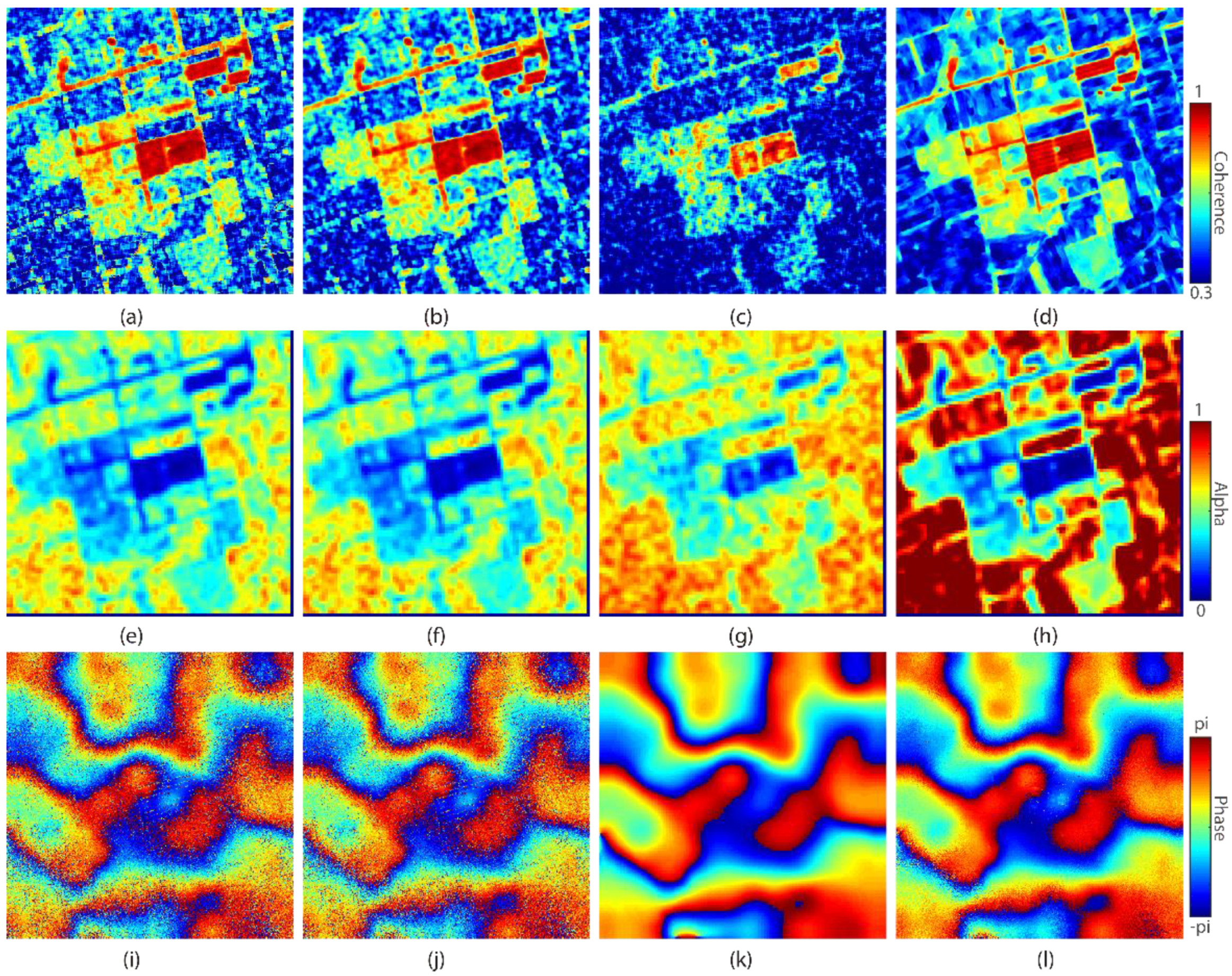
A result of the filtering process is shown in Figure 6. Clearly, the filtering results strongly depend on estimated parameters. For example, there is no significant difference between the Baran filter (i) and AGFC (j), because they use the same linear model and similar coherence magnitudes (>0.3) to estimate the filtering power (e and f). However, larger variances of coherence can be observed in (a) and (b). On the contrary, the coherence estimated by the new method (d) looks better for both edge preservation and magnitude because of the reduction of heterogeneity and also due to bias removal. More accurate coherence estimation in conjunction with the piece-wise model also leads to enhanced contrast in the filtering power (h), and therefore significant noise mitigation in (l). Although the filtering power of AGFP in (g) is still under-estimated and does not follow the noise features in Figure 5d, the filtered interferogram in (k) is smoother than those estimated from other methods. This is expected since AGFP is an iterative filtering process that removes noise from the previous result.

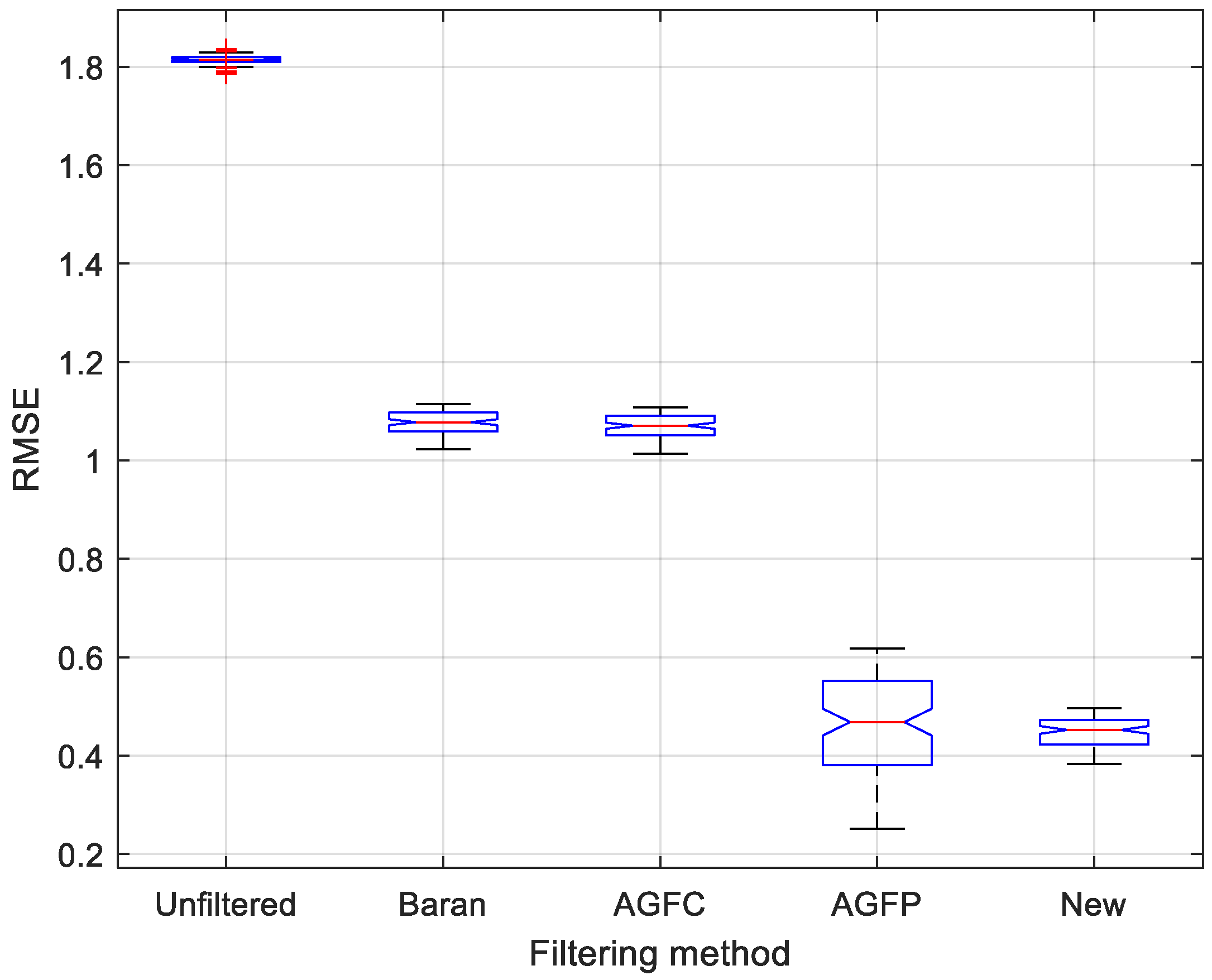
Quantitatively, the RMSEs between each filtered interferogram and true values are counted to evaluate the performance of different filters. As expected, Figure 6i,j have the largest RMSEs, at 1.10 rad and 1.09 rad, respectively. The RMSE of Figure 6l is 0.49 rad, slightly larger than that filtered by AGFP in Figure 6k (0.46 rad) because the iterative filtering enhanced smoothness at the cost of lost resolution. To further confirm this, the authors performed 100 iterations for each method using Equation (14), in which the universal multifractal technique can generate phase patterns with varying details. The results are shown in Figure 7. It can be seen that the Baran filter and AGFC under-estimate strong noise areas due to their biased filtering power and therefore have larger mean values for RMSEs. The iterative AGFP has a smaller mean but larger variance. The reason for this is that reduplicative filtering results in the loss of signal and consequent image blurring, and the degree of loss is related to the complexity of phase patterns in each simulation. In testing, the new filter performs better than all other filtering methods.

3.2. Real Data

Two SAR subsets acquired from Sentinel-1A with TOPS mode and TanDEM-X bistatic strip map mode were used to evaluate the performance of the new filter over incoherent and coherent scenarios, respectively. The results are shown in

Table 1. SAR dataset and study area.

Sensor	Track	Acquisition Date	Perp. Baseline	Imaging Area	Interferometric Feature	Mean Coherence
Sentinel-1A	128	30 July 2017	35 m	Jiuzhaigou, China	Incoherent	0.25
		11 August 2017
TanDEM-X	-	1 January 2013	286 m	Hong Kong, China	Coherent	0.76
		1 January 2013

. During pre-processing, the TOPS SAR images were co-registered, using precise satellite orbits and an external digital elevation model, followed by a refinement of shifts to estimate the azimuth offset between the two images. The TanDEM-X data was co-registered using a cross-correlation algorithm at a 0.1 pixel accuracy. Both datasets were compensated for topographic phase contribution before coherence estimation was conducted.

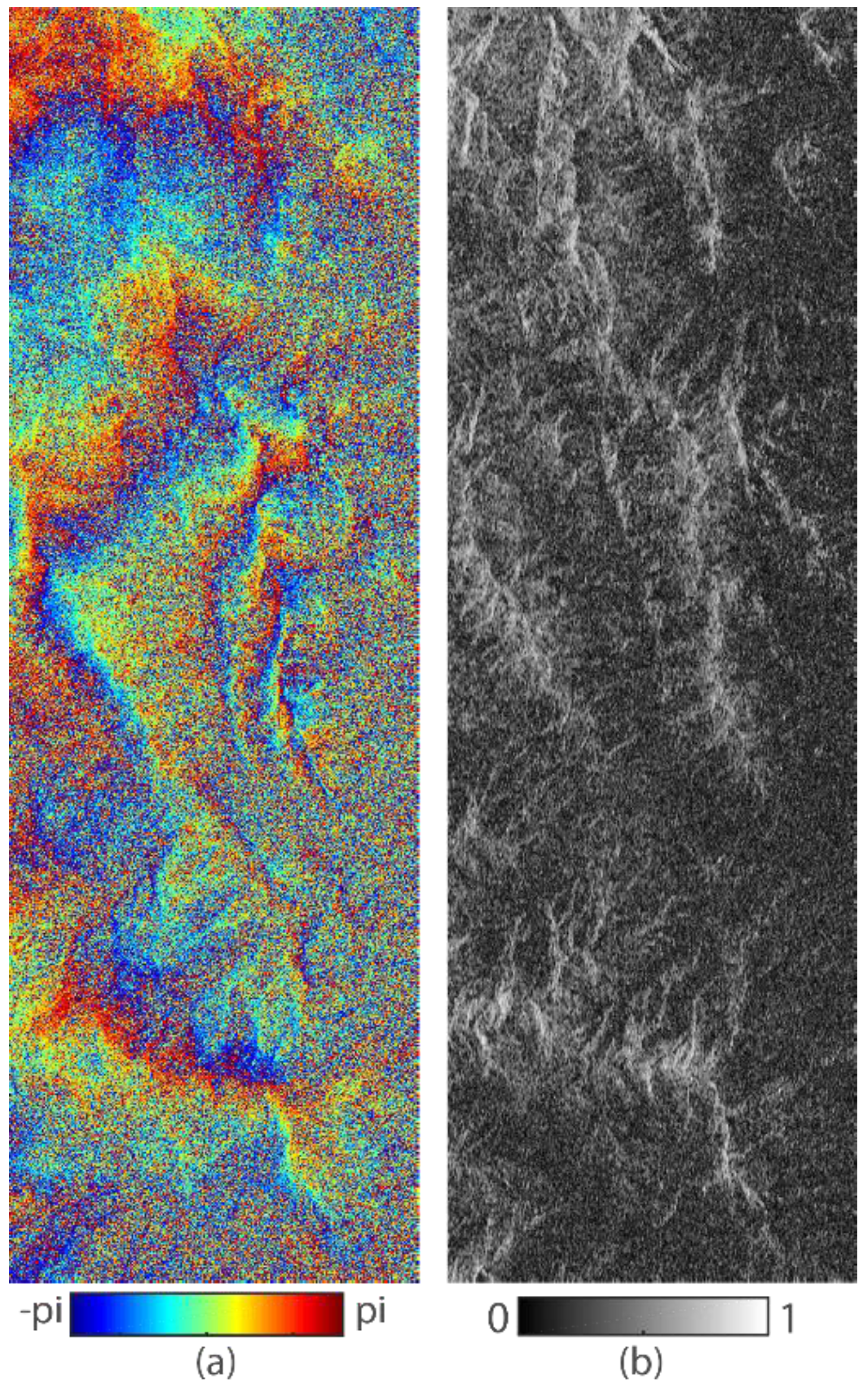
Figure 8a presents the original differential interferogram over the Jiuzhaigou area, where an earthquake with magnitude 7.0 occurred on 8 August 2017. After burst and sub-swath merging of the TOPS image, the non-linear deformation signals can be observed in the whole image. However, the low coherence in Figure 8b hinders a clear interpretation of the fringes. The purpose of this trial was to test the capability of the new filter to correct under-estimation of the Goldstein filtering power over an incoherent area.

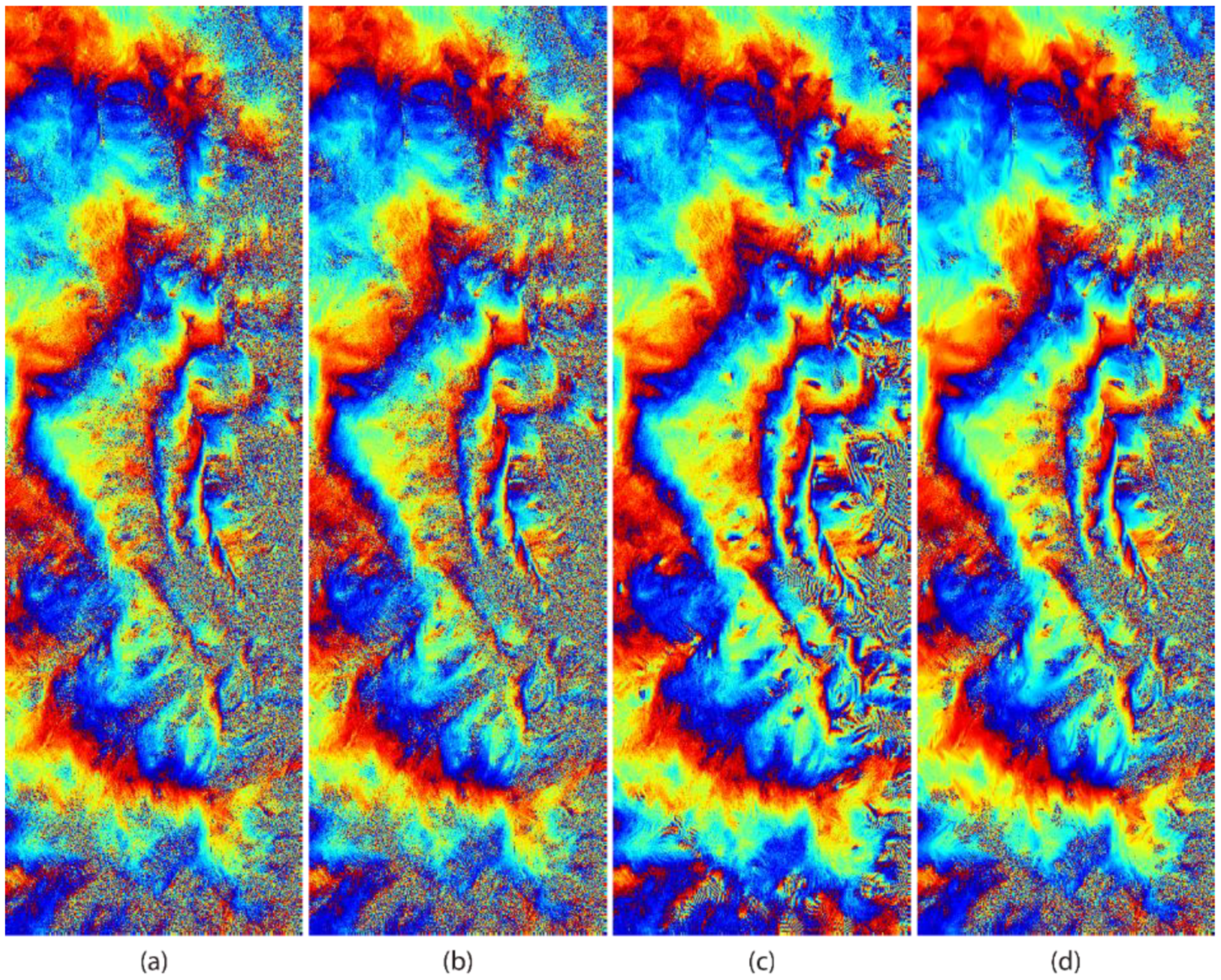
Compared with the Baran filter and AGFC in Figure 9a,b, the noise is significantly mitigated in interferograms from AGFP and for the new method in Figure 9c,d. This can also be confirmed from the sum of phase difference (SPD) [11] and the number of unwrapping residues in

Table 2. Statistics of SPD and residue reduction in interferograms estimated from different filters using Sentinel-1A data over the Jiuzhaigou area.

Method	$\mathit{SPD}(\times {10}^7)$	Residue Number	Residue Reduction (%)
Unfiltered	2.88	393,230	-
Baran	1.80	136,828	65.20
AGFC	1.72	125,197	68.16
AGFP	1.05	17,647	95.51
New	1.35	94,460	75.98

, in which a smaller SPD and residue value demonstrate the better performance of the new method for filtering for noise suppression [9,10]. Despite having minimum values for AGFP, it seems to yield spurious fringe patterns on the right in Figure 9c, where pure noise dominates. This issue is understandable as pure noise will contribute to the Fourier spectrum due to the missing estimation of spatial frequencies. This becomes an important drawback for iterative methods that cannot accurately threshold the boundary between completely decorrelated and low coherence areas. Therefore, the authors conclude that although the noise may be further reduced by iteration, the result shows that the bias removal for Goldstein filtering power can avoid artifacts and simultaneously mitigate noise.

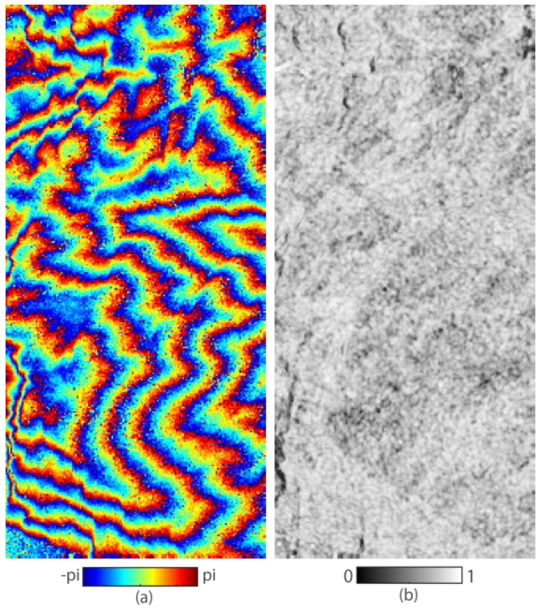
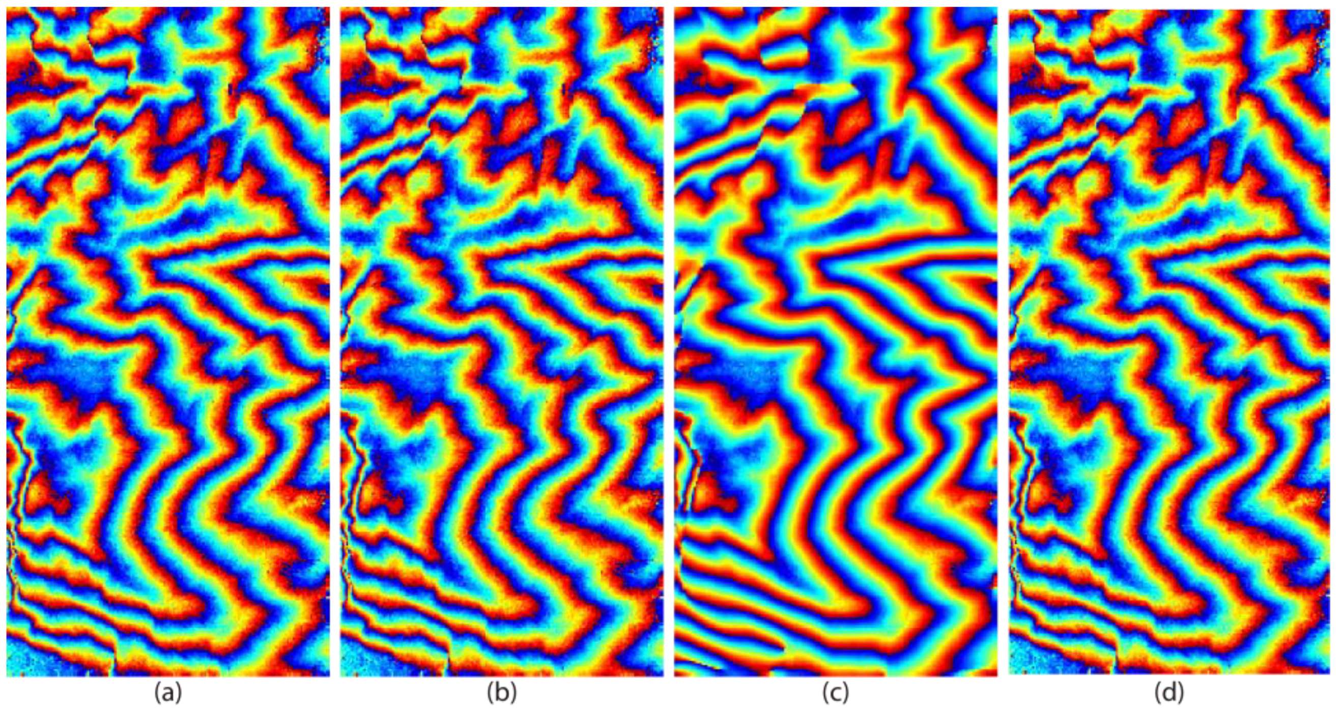
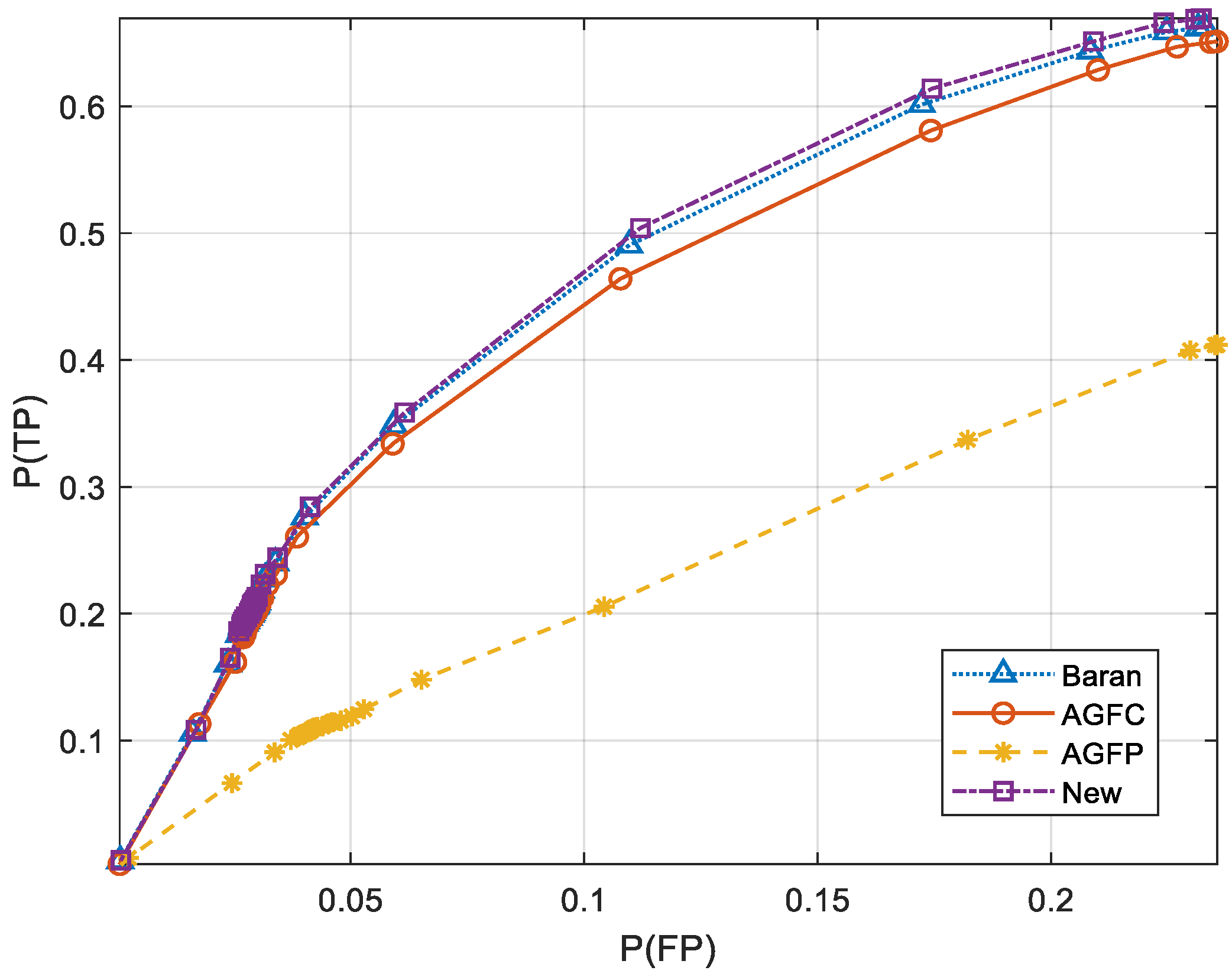
Finally, the authors present the results over a coherent area to demonstrate the effectiveness of the new filter for edge preservation. To this end, a mountainous area with very high coherence was selected and is shown in Figure 10. Figure 11 shows the filtered interferograms using different methods, where the differences among filters in Figure 11a,b,d are not distinguishable, while the result from AGFP seems to over-smooth the interferogram. This is identical to the previous case of synthetic data. The authors then deployed the receiver operating characteristics (ROC) to quantify the impact of the filtering effect on edge preservation. To do this, the Canny operator was first used to binarize the image. The edge of the original interferogram (Figure 10a) was assumed to be the positive instance and its complement the negative instance. Then, all true positive and false positive instances were counted for binary images estimated from each interferogram. By thresholding the Canny detector with various magnitudes for each filtered interferogram, the ROC curves were constructed as shown in Figure 12. The more the ROC curves toward the upper left, the better the edge preservation. The curve estimated from ADFP is located in the bottom right corner, showing the worst performance for the quality of edge preservation. It is also important to note similar ROC features for other methods in the case. This is due to the fact that there is no bias on high coherence levels in Figure 2 and weak differences between the linear model and piece-wise model in Figure 3, which results in similar filtering powers.

4. Conclusions

Bias correction for Goldstein filtering power is crucial for interferometric data post-processing and the subsequent multitemporal analysis. Having an accurate filtering power can mitigate both under- and over-estimation of phase noise in interferograms showing different features. This paper presents a method for bias removal from accurate coherence estimation and model development that links coherence and filtering power. Based on the weighted coherence estimator that combines a second kind statistic with an Anderson-Darling test statistic, the unbiased sample coherence with a better spatial distribution is deduced. Driven by sample coherence, the optimal filtering power for each filtered patch is then determined from a piece-wise model, which detects the best filtering performance under each coherence level using a Monte Carlo simulation. The authors finally evaluate the effectiveness of the bias corrected Goldstein filter using both synthetic and real data and compare it against other adaptive filters that fix filter power by biased coherence, unbiased coherence with regular statistics, and iteration. A series of experimental results validated the improvements resulting from the newly developed method for noise reduction and edge preservation.

References

- Shi, X.; Jiang, H.; Zhang, L.; Liao, M. Landslide displacement monitoring with split-bandwidth interferometry: A case study of the shuping landslide in the three gorges area. Remote Sens. 2017, 9, 937. [Google Scholar] [CrossRef]
- Solberg, S.; Astrup, R.; Breidenbach, J.; Nilsen, B.; Weydahl, D. Monitoring spruce volume and biomass with insar data from tandem-x. Remote Sens. Environ. 2013, 139, 60–67. [Google Scholar] [CrossRef]
- Jiang, M.; Yong, B.; Tian, X.; Malhotra, R.; Hu, R.; Li, Z.; Yu, Z.; Zhang, X. The potential of more accurate insar covariance matrix estimation for land cover mapping. ISPRS J. Photogramm. Remote Sens. 2017, 126, 120–128. [Google Scholar] [CrossRef]
- Romeiser, R.; Runge, H. Theoretical evaluation of several possible along-track insar modes of terrasar-x for ocean current measurements. IEEE Trans. Geosci. Remote Sens. 2007, 45, 21–35. [Google Scholar] [CrossRef]
- Zhou, Y.; Thomas, M.Y.; Parsons, B.; Walker, R.T. Time-dependent postseismic slip following the 1978 m w 7.3 tabas-e-golshan, iran earthquake revealed by over 20 years of esa insar observations. Earth Planet. Sci. Lett. 2018, 483, 64–75. [Google Scholar] [CrossRef]
- Zebker, H.A.; Villasenor, J. Decorrelation in interferometric radar echoes. IEEE Trans. Geosci. Remote Sens. 1992, 30, 950–959. [Google Scholar] [CrossRef] [Green Version]
- Goldstein, R.M.; Werner, C.L. Radar interferogram filtering for geophysical applications. Geophys. Res. Lett. 1998, 25, 4035–4038. [Google Scholar] [CrossRef] [Green Version]
- Hooper, A.; Zebker, H.A. Phase unwrapping in three dimensions with application to insar time series. J. Opt. Soc. Am. A Opt. Image Sci. Vis. 2007, 24, 2737–2747. [Google Scholar] [CrossRef] [PubMed]
- Baran, I.; Stewart, M.P.; Kampes, B.M.; Perski, Z.; Lilly, P. A modification to the goldstein radar interferogram filter. IEEE Trans. Geosci. Remote Sens. 2003, 41, 2114–2118. [Google Scholar] [CrossRef]
- Li, Z.; Ding, X.; Huang, C.; Zhu, J.; Chen, Y. Improved filtering parameter determination for the goldstein radar interferogram filter. ISPRS J. Photogramm. Remote Sens. 2008, 63, 621–634. [Google Scholar] [CrossRef]
- Jiang, M.; Ding, X.; Li, Z.; Tian, X.; Zhu, W.; Wang, C.; Xu, B. The improvement for baran phase filter derived from unbiased insar coherence. IEEE J. Sel. Top. Appl. Earth Obs. Remote Sens. 2014, 7, 3002–3010. [Google Scholar] [CrossRef]
- Wang, B.-H.; Zhao, C.-Y.; Liu, Y.-Y. An improved sar interferogram denoising method based on principal component analysis and the goldstein filter. Remote Sens. Lett. 2018, 9, 81–90. [Google Scholar] [CrossRef]
- Zhao, C.; Zhang, Q.; Ding, X.; Zhang, J. An iterative goldstein sar interferogram filter. Int. J. Remote Sens. 2012, 33, 3443–3455. [Google Scholar] [CrossRef]
- Mestre-Quereda, A.; Lopez-Sanchez, J.M.; Selva, J.; Gonzalez, P.J. An improved phase filter for differential sar interferometry based on an iterative method. IEEE Trans. Geosci. Remote Sens. 2018, 56, 4477–4491. [Google Scholar] [CrossRef]
- Touzi, R.; Lopes, A.; Bruniquel, J.; Vachon, P.W. Coherence estimation for sar imagery. IEEE Trans. Geosci. Remote Sens. 1999, 37, 135–149. [Google Scholar] [CrossRef]
- Jiang, M.; Ding, X.; Li, Z. Hybrid approach for unbiased coherence estimation for multitemporal insar. IEEE Trans. Geosci. Remote Sens. 2014, 52, 2459–2473. [Google Scholar] [CrossRef]
- Fan, J.; Farmen, M.; Gijbels, I. Local maximum likelihood estimation and inference. J. R. Stat. Soc. Ser. B 1998, 60, 591–608. [Google Scholar] [CrossRef] [Green Version]
- Pettitt, A.N. A two-sample anderson-darling rank statistic. Biometrika 1976, 63, 161–168. [Google Scholar]
- Darling, D. The kolmogorov-smirnov, cramer-von mises tests. Ann. Math. Stat. 1957, 28, 823–838. [Google Scholar] [CrossRef]
- Rother, C.; Kolmogorov, V.; Blake, A. Grabcut: Interactive Foreground Extraction Using Iterated Graph Cuts; ACM Transactions on Graphics (TOG); ACM: New York, NY, USA, 2004; pp. 309–314. [Google Scholar]
- Ferretti, A.; Fumagalli, A.; Novali, F.; Prati, C.; Rocca, F.; Rucci, A. A new algorithm for processing interferometric data-stacks: Squeesar. IEEE Trans. Geosci. Remote Sens. 2011, 49, 3460–3470. [Google Scholar] [CrossRef]
- Jiang, M.; Ding, X.; Hanssen, R.F.; Malhotra, R.; Chang, L. Fast statistically homogeneous pixel selection for covariance matrix estimation for multitemporal insar. IEEE Trans. Geosci. Remote Sens. 2015, 53, 1213–1224. [Google Scholar] [CrossRef]
- Nicolas, J.M. Introduction to second kind statistics: Application of log-moments and log-cumulants to sar image law analysis. Trait. Signal 2002, 19, 139–168. [Google Scholar]
- Abdelfattah, R.; Nicolas, J.M. Interferometric sar coherence magnitude estimation using second kind statistics. IEEE Trans. Geosci. Remote Sens. 2006, 44, 1942–1953. [Google Scholar] [CrossRef]
- Pecknold, S.; Lovejoy, S.; Schertzer, D.; Hooge, C.; Malouin, J. The simulation of universal multifractals. In Cellular Automata: Prospects in Astronomy and Astrophysics; Perdang, J.M., Lejeune, A., Eds.; World Scientific Pub Co Inc.: Singapore, 1993; pp. 228–267. [Google Scholar]
- Lee, J.-S.; Pottier, E. Polarimetric Radar Imaging: From Basics to Applications; CRC Press LLC: Boca Raton, FL, USA, 2009; Volume 142. [Google Scholar]
Figure 1.
Similarity measurement using the patch-based Anderson-Darling test: (a) The procedure of AD estimation; (b) some similar patches (green) with respect to the reference patch (red); (c) the corresponding AD values of the whole window.
Figure 2.
Bias of coherence estimators.
Figure 3.
The best filtering power under each coherence level. The dashed line denotes the empirical model presented in [9].
Figure 4.
Bias corrected adaptive Goldstein filter diagram.
Figure 5.
Synthetic data with 400 400 pixels. (a) Noise-free SAR intensity; (b) original coherence; (c) noise-free interferogram; and (d) noise-added interferogram after the conjugation operator .
Figure 6.
The results estimated from different methods. Each column corresponds to a filtering procedure: first (Baran filter), second (AGFC), third (AGFP), and last (new filter). Each row corresponds to a parameter: first (coherence), second (filtering power), and third (filtered phase).
Figure 7.
The boxplot of RMSEs between the truth and interferogram filtered by different methods.
Figure 8.
Interferometric feature over Jiuzhaigou area, China. (a) Phase and (b) coherence.
Figure 9.
Interferogram filtering over incoherent area. (a) Baran filter; (b) AGFC; (c) AGFP; (d) New.
Figure 10.
Interferometric feature over a mountain area, Hong Kong. (a) Phase and (b) coherence.
Figure 11.
Interferogram filtering over coherent area. (a) Baran filter; (b) AGFC; (c) AGFP; (d) New.
Figure 12.
The ROC curves for evaluating the filtering performances on edge preservation over the coherent area.