Mining Hard Negative Samples for SAR-Optical Image Matching Using Generative Adversarial Networks


Abstract
: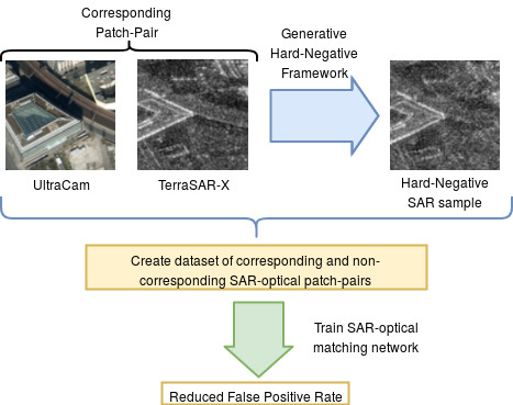
1. Introduction
2. Generative Framework for Hard Negative Mining
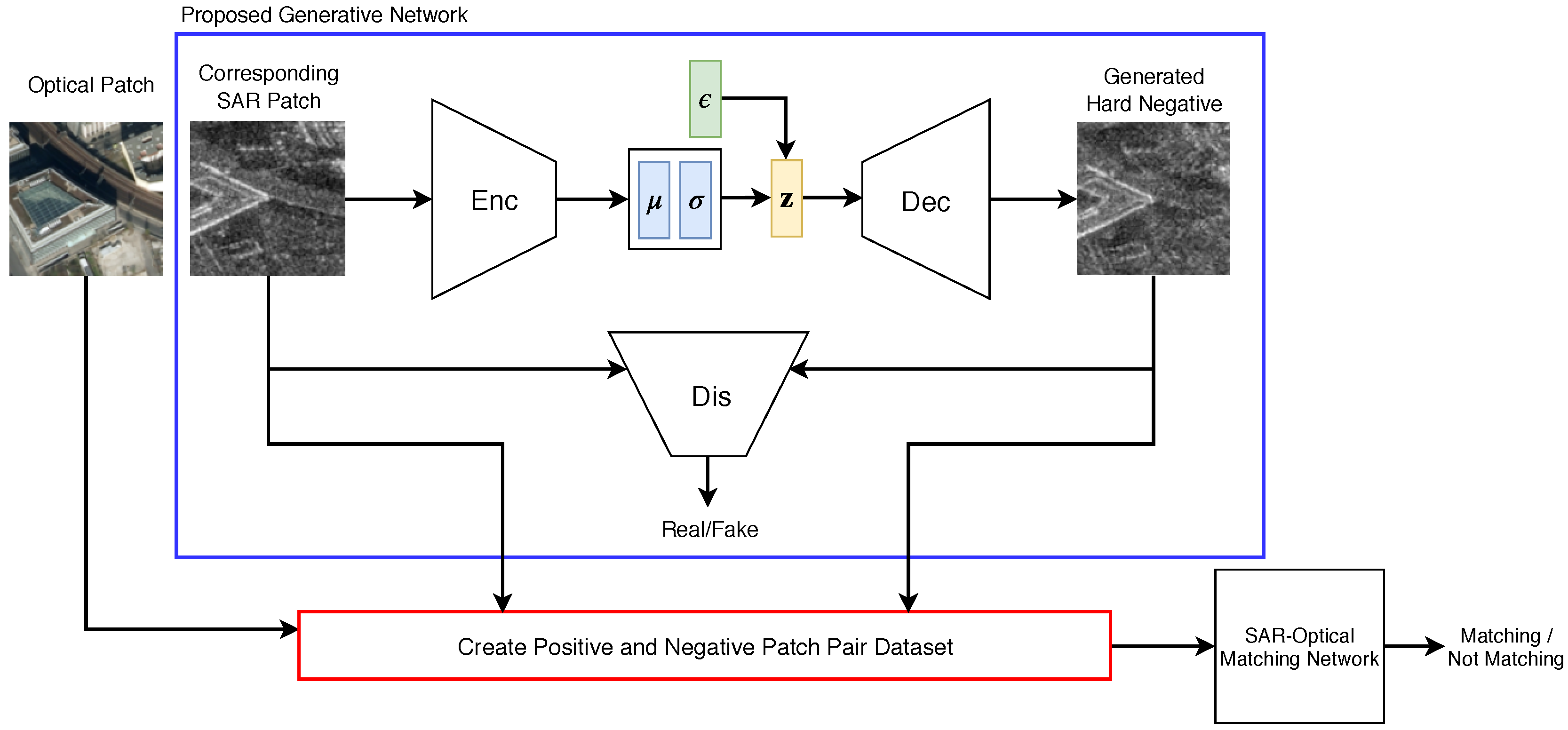
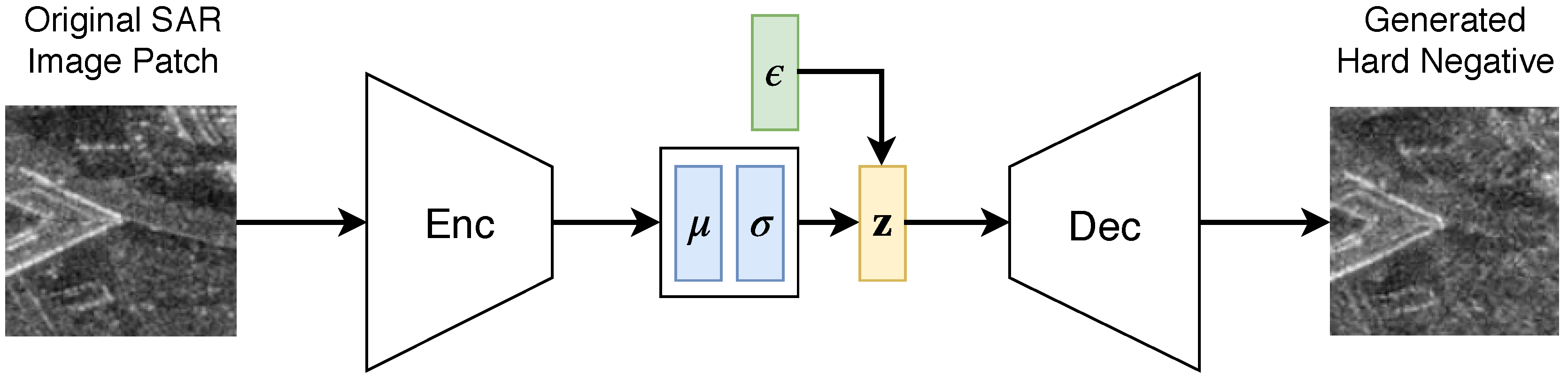
2.1. Proposed Generative Architecture
2.1.1. Generator
2.1.2. Discriminator
2.2. Training Procedure
2.2.1. Progressive Growing
2.2.2. WGAN-GP Loss
2.2.3. Additional Training Details
| Algorithm 1: Training our Hard Negative GAN |
,, |
2.3. Generating Hard Negative Samples
3. Experiments and Results
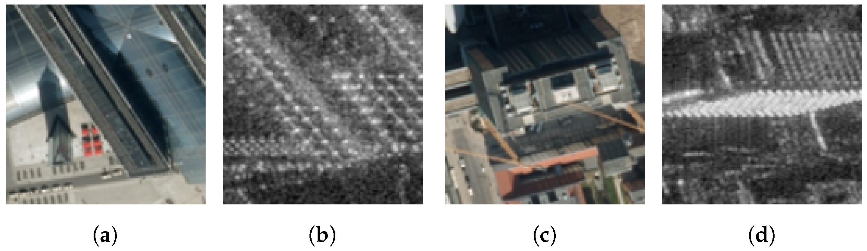
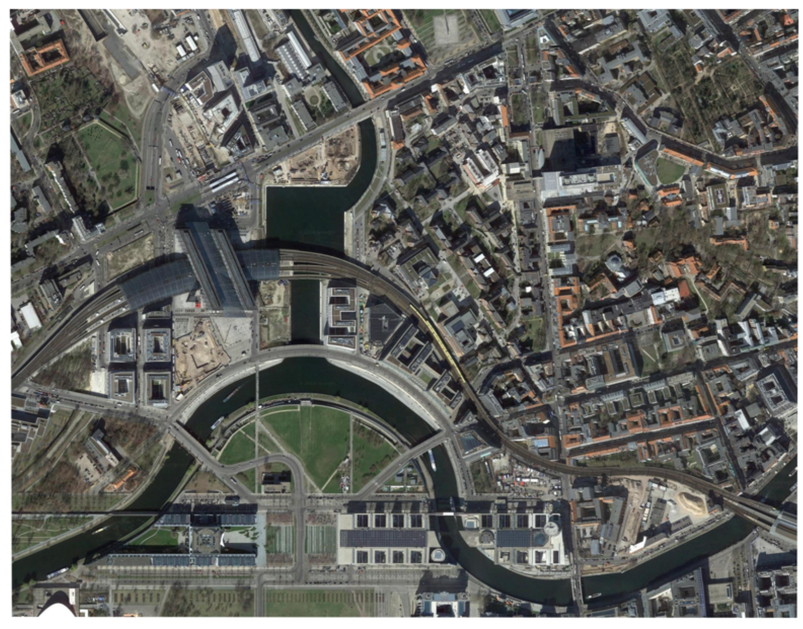
3.1. Dataset
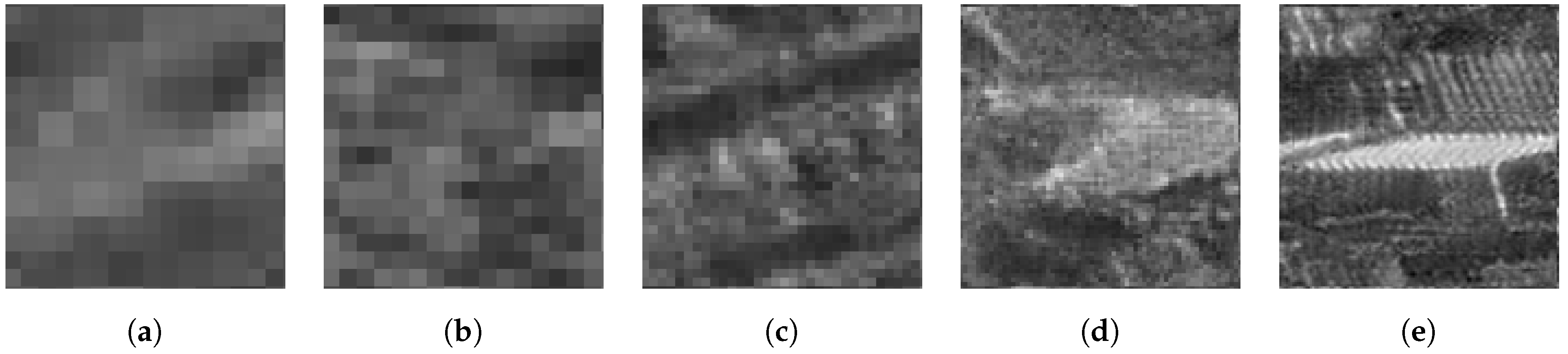
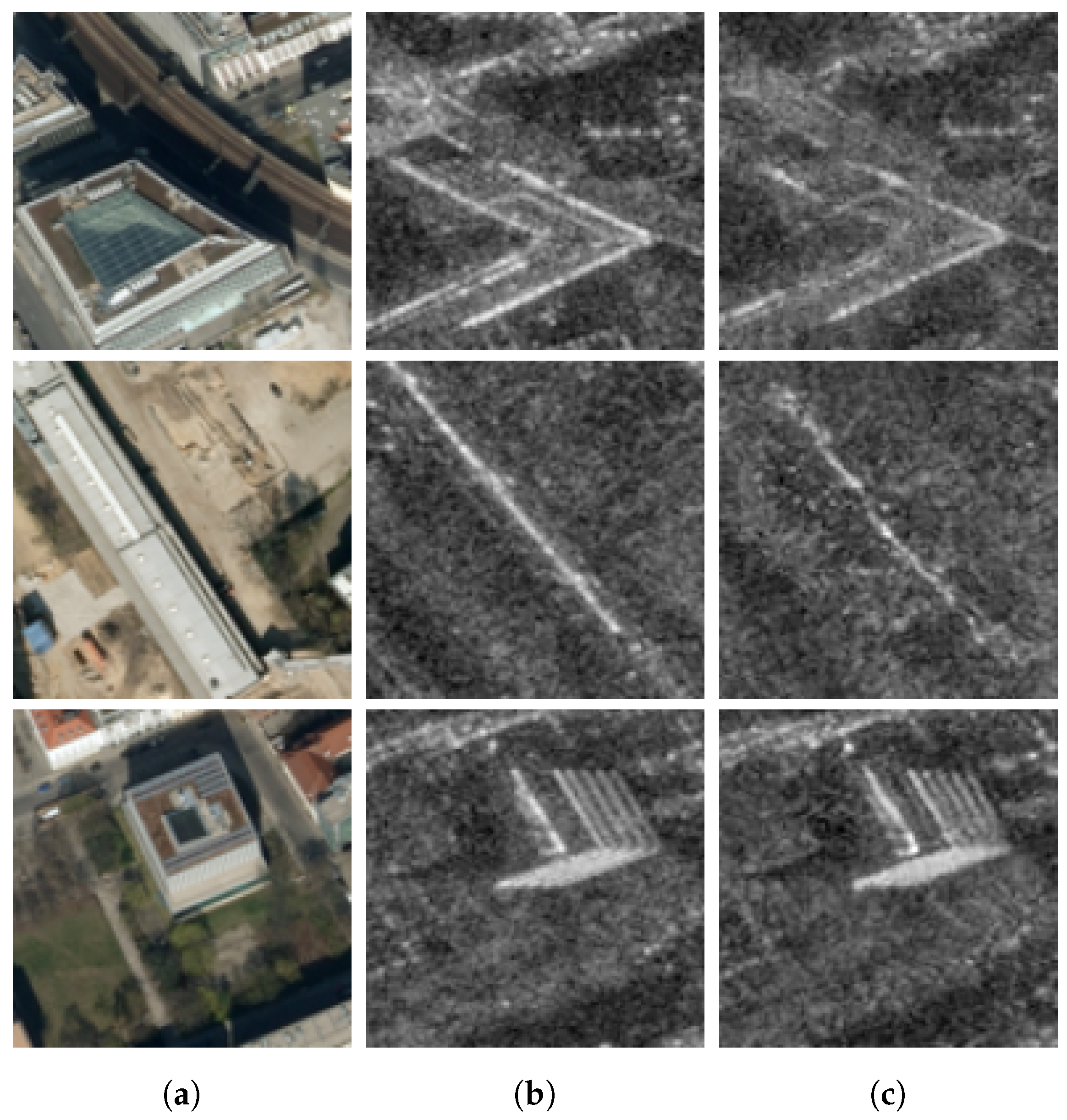
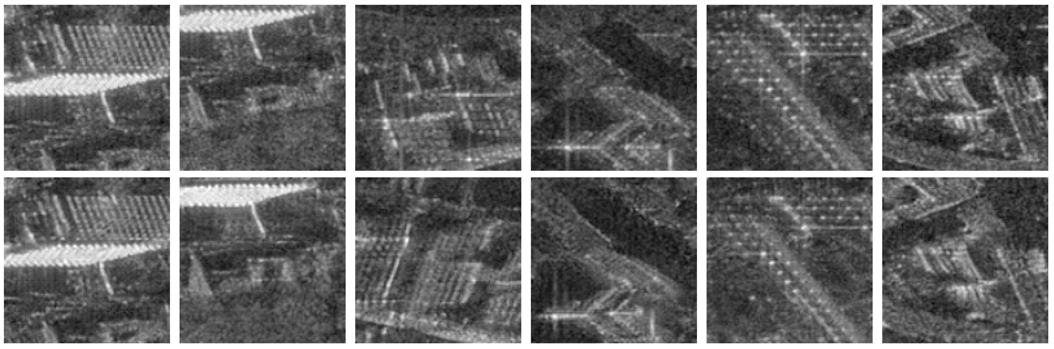
3.2. Qualitative Evaluation of Generated Negative Samples
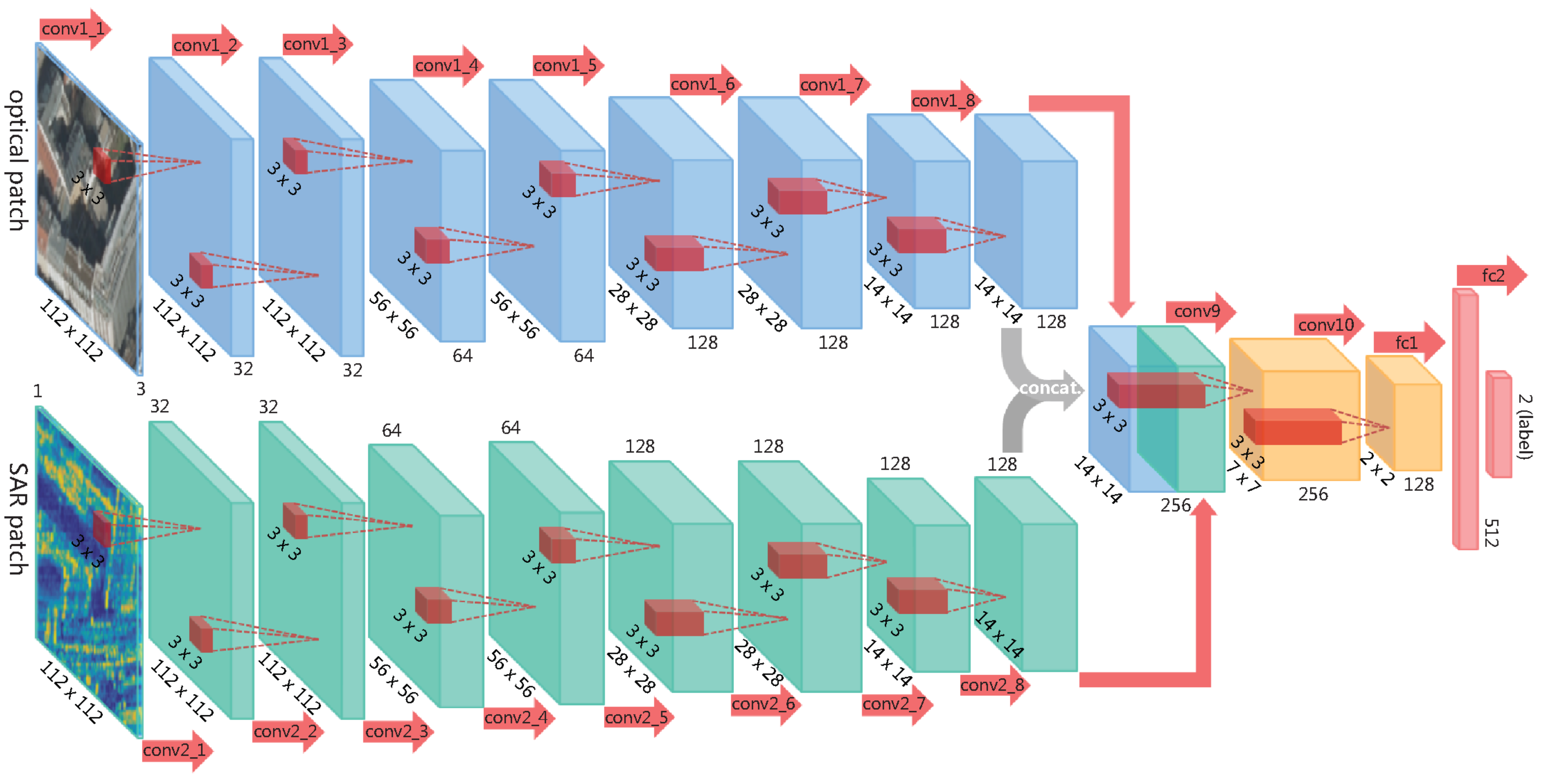
3.3. Matching SAR and Optical Images
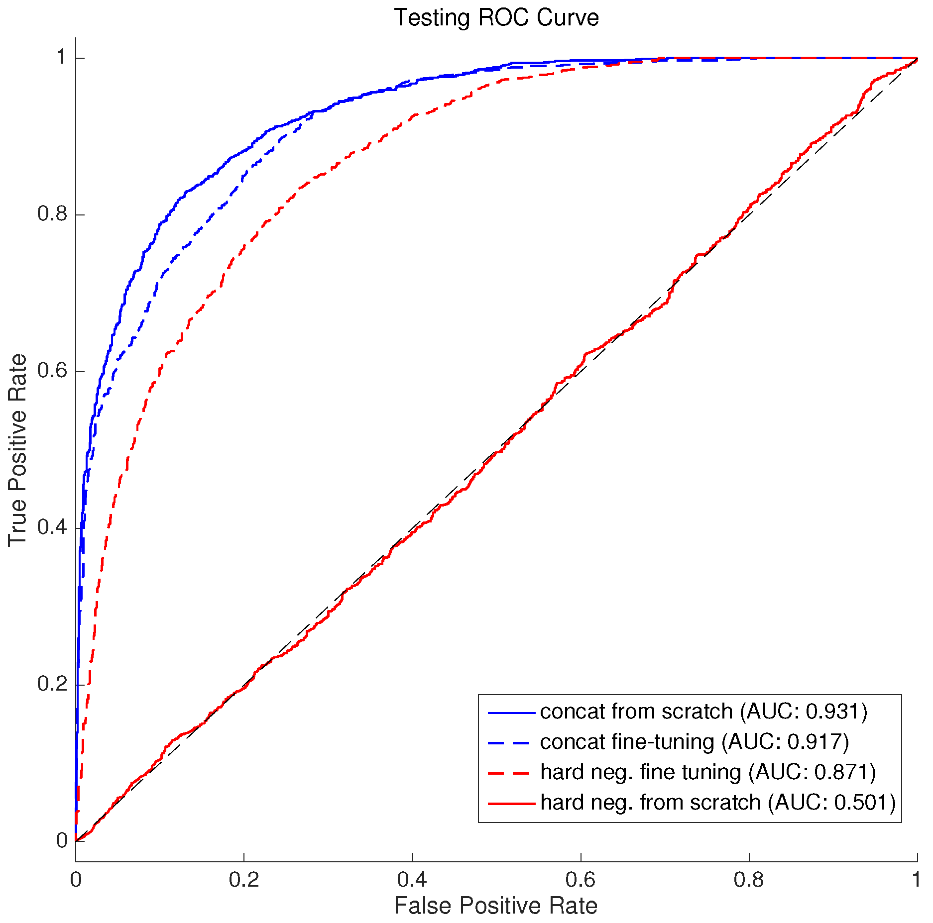
3.4. Effect of a Hard Negative Inclusion Method
- Fine-tuning with generated hard negatives,
- Fine-tuning with concatenated dataset,
- Training from scratch with generated hard negatives,
- Training from scratch with concatenated dataset.
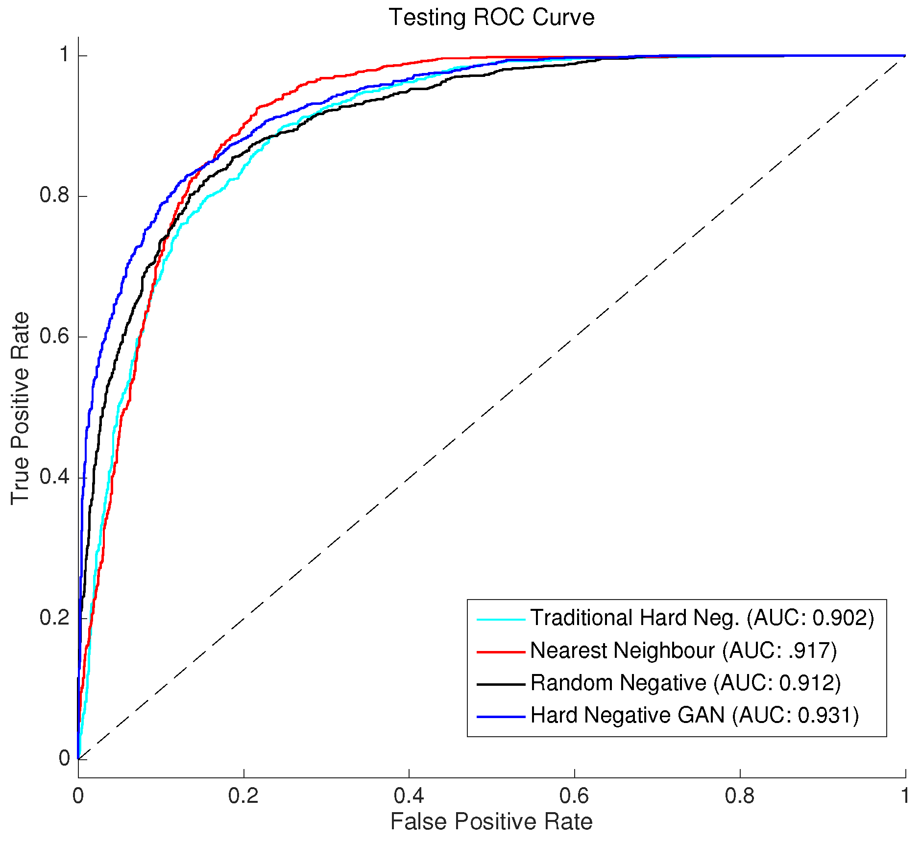
3.5. Comparison to Existing Approaches
4. Discussion
4.1. Generative Ability
4.2. Effects of Data Inclusion Approach
4.3. SAR-Optical Matching Performance
4.4. Comments on Computational Overhead
5. Conclusions
Author Contributions
Funding
Conflicts of Interest
References
- Schmitt, M.; Zhu, X.X. Data Fusion and Remote Sensing—An Ever-Growing Relationship. IEEE Geosci. Remote Sens. Mag. 2016, 4, 6–23. [Google Scholar] [CrossRef]
- Schmitt, M.; Tupin, F.; Zhu, X.X. Fusion of SAR and optical remote sensing data—Challenges and recent trends. In Proceedings of the 2017 IEEE International Geoscience and Remote Sensing Symposium, Fort Worth, TX, USA, 23–28 July 2017; pp. 5458–5461. [Google Scholar]
- Ye, Y.; Shan, J.; Bruzzone, L.; Shen, L. Robust Registration of Multimodal Remote Sensing Images Based on Structural Similarity. IEEE Trans. Geosci. Remote Sens. 2017, 55, 2941–2958. [Google Scholar] [CrossRef]
- Li, J.; Hu, Q.; Ai, M. RIFT: Multi-modal Image Matching Based on Radiation-invariant Feature Transform. arXiv, 2018; arXiv:1804.09493. [Google Scholar]
- Qiu, C.; Schmitt, M.; Zhu, X.X. Towards automatic SAR-optical stereogrammetry over urban areas using very high resolution imagery. ISPRS J. Photogramm. Remote Sens. 2018, 138, 218–231. [Google Scholar] [CrossRef] [PubMed]
- Palubinskas, G.; Reinartz, P.; Bamler, R. Image acquisition geometry analysis for the fusion of optical and radar remote sensing data. Int. J. Image Data Fusion 2010, 1, 271–282. [Google Scholar] [CrossRef] [Green Version]
- Balntas, V.; Johns, E.; Tang, L.; Mikolajczyk, K. PN-Net: Conjoined triple deep network for learning local image descriptors. arXiv, 2016; arXiv:1601.05030. [Google Scholar]
- Yi, K.M.; Trulls, E.; Lepetit, V.; Fua, P. Lift: Learned invariant feature transform. In European Conference on Computer Vision; Springer: Cham, Switzerland, 2016; pp. 467–483. [Google Scholar]
- Zagoruyko, S.; Komodakis, N. Deep compare: A study on using convolutional neural networks to compare image patches. Comput. Vis. Image Underst. 2017, 164, 38–55. [Google Scholar] [CrossRef]
- Han, X.; Leung, T.; Jia, Y.; Sukthankar, R.; Berg, A.C. Matchnet: Unifying feature and metric learning for patch-based matching. In Proceedings of the IEEE Conference on Computer Vision and Pattern Recognition, Boston, MA, USA, 7–12 June 2015; pp. 3279–3286. [Google Scholar]
- Zhu, X.X.; Tuia, D.; Mou, L.; Xia, G.S.; Zhang, L.; Xu, F.; Fraundorfer, F. Deep Learning in Remote Sensing: A Comprehensive Review and List of Resources. IEEE Geosci. Remote Sens. Mag. 2017, 5, 8–36. [Google Scholar] [CrossRef] [Green Version]
- Merkle, N.; Luo, W.; Auer, S.; Müller, R.; Urtasun, R. Exploiting Deep Matching and SAR Data for the Geo-Localization Accuracy Improvement of Optical Satellite Images. Remote Sens. 2017, 9, 586. [Google Scholar] [CrossRef]
- Mou, L.; Schmitt, M.; Wang, Y.; Zhu, X. A CNN for the Identification of Corresponding Patches in SAR and Optical Imagery of Urban Scenes. In Proceedings of the 2017 Joint Urban Remote Sensing Event (JURSE), Dubai, UAE, 6–8 March 2017. [Google Scholar]
- Hughes, L.H.; Schmitt, M.; Mou, L.; Wang, Y.; Zhu, X.X. Identifying Corresponding Patches in SAR and Optical Images With a Pseudo-Siamese CNN. IEEE Geosci. Remote Sens. Lett. 2018, 15, 784–788. [Google Scholar] [CrossRef] [Green Version]
- Merkle, N.; Auer, S.; Müller, R.; Reinartz, P. Exploring the Potential of Conditional Adversarial Networks for Optical and SAR Image Matching. IEEE J-STARS 2018, 11, 1811–1820. [Google Scholar] [CrossRef]
- Sung, K.K.; Poggio, T. Example-based learning for view-based human face detection. IEEE Trans. Pattern Anal. Mach. Intell. 1998, 20, 39–51. [Google Scholar] [CrossRef] [Green Version]
- Wang, Y.; Zhu, X.; Zeisl, B.; Pollefeys, M. Fusing meter-resolution 4-D InSAR point clouds and optical images for semantic urban infrastructure monitoring. IEEE Trans. Geosci. Remote Sens. 2016, 55, 14–26. [Google Scholar] [CrossRef]
- Auer, S.; Hornig, I.; Schmitt, M.; Reinartz, P. Simulation-based Interpretation and Alignment of High-Resolution Optical and SAR Images. IEEE J-STARS 2017, 10, 4779–4793. [Google Scholar] [CrossRef]
- Wang, Y.; Zhu, X.X. The SARptical Dataset for Joint Analysis of SAR and Optical Image in Dense Urban Area. arXiv, 2018; arXiv:1801.07532. [Google Scholar]
- Ding, J.; Chen, B.; Liu, H.; Huang, M. Convolutional neural network with data augmentation for SAR target recognition. IEEE Geosci. Remote Sens. Lett. 2016, 13, 364–368. [Google Scholar] [CrossRef]
- Zheng, Z.; Zheng, L.; Yang, Y. Unlabeled samples generated by gan improve the person re-identification baseline in vitro. arXiv, 2017; arXiv:1701.07717. [Google Scholar]
- Ley, A.; d’Hondt, O.; Valade, S.; Hänsch, R.; Hellwich, O. Exploiting GAN-based SAR to optical image transcoding for improved classification via deep learning. In Proceedings of the 12th European Conference on Synthetic Aperture Radar, Aachen, Germany, 4–7 June 2018; pp. 396–401. [Google Scholar]
- Wang, P.; Li, S.; Pan, R. Incorporating GAN for Negative Sampling in Knowledge Representation Learning. In Proceedings of the Thirty-Second AAAI Conference on Artificial Intelligence, New Orleans, LA, USA, 2–7 February 2018. [Google Scholar]
- Marmanis, D.; Yao, W.; Adam, F.; Datcu, M.; Reinartz, P.; Schindler, K.; Wegner, J.D.; Stilla, U. Artificial generation of big data for improving image classification: A generative adversarial network approach on SAR data. arXiv, 2017; arXiv:1711.02010. [Google Scholar]
- Ao, D.; Dumitru, C.O.; Schwarz, G.; Datcu, M. Dialectical GAN for SAR Image Translation: From Sentinel-1 to TerraSAR-X. arXiv, 2018; arXiv:1807.07778. [Google Scholar]
- Karras, T.; Aila, T.; Laine, S.; Lehtinen, J. Progressive Growing of GANs for Improved Quality, Stability, and Variation. arXiv, 2018; arXiv:1710.10196. [Google Scholar]
- Khan, S.H.; Hayat, M.; Barnes, N. Adversarial Training of Variational Auto-encoders for High Fidelity Image Generation. arXiv, 2018; arXiv:1804.10323. [Google Scholar]
- Larsen, A.B.L.; Sønderby, S.K.; Larochelle, H.; Winther, O. Autoencoding beyond pixels using a learned similarity metric. arXiv, 2015; arXiv:1512.09300. [Google Scholar]
- Goodfellow, I.; Bengio, Y.; Courville, A. Deep Learning; MIT Press: Cambridge, MA, USA, 2016. [Google Scholar]
- Gulrajani, I.; Ahmed, F.; Arjovsky, M.; Dumoulin, V.; Courville, A.C. Improved training of Wasserstein GANs. In Proceedings of the Advances in Neural Information Processing Systems, Long Beach, CA, USA, 4–9 December 2017; pp. 5769–5779. [Google Scholar]
- Theis, L.; van den Oord, A.; Bethge, M. A note on the evaluation of generative models. In Proceedings of the 2016 International Conference on Learning Representations, San Juan, Puerto Rico, 2–4 May 2016. [Google Scholar]
- Sung, K.K. Learning and Example Selection for Object and Pattern Detection; Computer Science and Artificial Intelligence Lab: Cambridge, MA, USA, 1996. [Google Scholar]
- Jiang, F. SVM-Based Negative Data Mining to Binary Classification. Ph.D. Thesis, Georgia State University, Atlanta, GA, USA, 2006. [Google Scholar]


| Encoder | Act. | Output Shape |
| Conv 1 × 1 | LReLU | N × 1 × 128 × 128 |
| Conv 3 × 3 | LReLU | N × 128 × 128 × 128 |
| Conv 3 × 3 | LReLU | N × 256 × 128 × 128 |
| Downsample | - | N × 256 × 64 × 64 |
| Conv 3 × 3 | LReLU | N × 256 × 64 × 64 |
| Conv 3 × 3 | LReLU | N × 512 × 64 × 64 |
| Downsample | - | N × 512 × 32 × 32 |
| Conv 3 × 3 | LReLU | N × 512 × 32 × 32 |
| Conv 3 × 3 | LReLU | N × 512 × 32 × 32 |
| Downsample | - | N × 512 × 16 × 16 |
| Conv 3 × 3 | LReLU | N × 512 × 16 × 16 |
| Conv 3 × 3 | LReLU | N × 512 × 16 × 16 |
| Downsample | - | N × 512 × 8 × 8 |
| Conv 3 × 3 | LReLU | N × 512 × 8 × 8 |
| Conv 3 × 3 | LReLU | N × 512 × 8 × 8 |
| Downsample | - | N × 512 × 4 × 4 |
| Conv 3 × 3 | LReLU | N × 512 × 4 × 4 |
| Conv 4 × 4 | LReLU | N × 512 × 1 × 1 |
| Fully Connected | Linear | N × 1024 × 1 × 1 |
| Mean | Split | N × 512 × 1 × 1 |
| Std. Deviation | N × 512 × 1 × 1 | |
| Decoder | Act. | Output Shape |
| Latent Vector | - | N × 512 × 1 × 1 |
| Conv 4 × 4 | LReLU | N × 512 × 4 × 4 |
| Conv 3 × 3 | LReLU | N × 512 × 4 × 4 |
| Upsample | - | N × 512 × 8 × 8 |
| Conv 3 × 3 | LReLU | N × 512 × 8 × 8 |
| Conv 3 × 3 | LReLU | N × 512 × 8 × 8 |
| Upsample | - | N × 512 × 16 × 16 |
| Conv 3 × 3 | LReLU | N × 512 × 16 × 16 |
| Conv 3 × 3 | LReLU | N × 512 × 16 × 16 |
| Upsample | - | N × 512 × 32 × 32 |
| Conv 3 × 3 | LReLU | N × 512 × 32 × 32 |
| Conv 3 × 3 | LReLU | N × 512 × 32 × 32 |
| Upsample | - | N × 512 × 64 × 64 |
| Conv 3 × 3 | LReLU | N × 256 × 64 × 64 |
| Conv 3 × 3 | LReLU | N × 256 × 64 × 64 |
| Upsample | - | N × 256 × 128 × 128 |
| Conv 3 × 3 | LReLU | N × 128 × 128 × 128 |
| Conv 3 × 3 | LReLU | N × 128 × 128 × 128 |
| Conv 1 × 1 | Linear | N × 1 × 128 × 128 |
| Discriminator | Act. | Output Shape |
|---|---|---|
| Conv 1 × 1 | LReLU | N × 1 × 128 × 128 |
| Conv 3 × 3 | LReLU | N × 128 × 128 × 128 |
| Conv 3 × 3 | LReLU | N × 256 × 128 × 128 |
| Downsample | - | N × 256 × 64 × 64 |
| Conv 3 × 3 | LReLU | N × 256 × 64 × 64 |
| Conv 3 × 3 | LReLU | N × 512 × 64 × 64 |
| Downsample | - | N × 512 × 32 × 32 |
| Conv 3 × 3 | LReLU | N × 512 × 32 × 32 |
| Conv 3 × 3 | LReLU | N × 512 × 32 × 32 |
| Downsample | - | N × 512 × 16 × 16 |
| Conv 3 × 3 | LReLU | N × 512 × 16 × 16 |
| Conv 3 × 3 | LReLU | N × 512 × 16 × 16 |
| Downsample | - | N × 512 × 8 × 8 |
| Conv 3 × 3 | LReLU | N × 512 × 8 × 8 |
| Conv 3 × 3 | LReLU | N × 512 × 8 × 8 |
| Downsample | - | N × 512 × 4 × 4 |
| Mini-batch Std. Dev. | - | N × 513 × 4 × 4 |
| Conv 3 × 3 | LReLU | N × 512 × 4 × 4 |
| Conv 4 × 4 | LReLU | N × 512 × 1 × 1 |
| Fully Connected | Linear | N × 1 × 1 × 1 |
| Method | Precision | Recall | Acc. (5% FPR) | Max Acc. | Max Acc. FPR |
|---|---|---|---|---|---|
| Random | 0.83 | 0.84 | 0.76 | 0.83 | 0.16 |
| Nearest Neighbour | 0.77 | 0.96 | 0.70 | 0.85 | 0.21 |
| Traditional Hard Neg. | 0.79 | 0.89 | 0.72 | 0.83 | 0.19 |
| Proposed Approach | 0.83 | 0.87 | 0.81 | 0.86 | 0.13 |
© 2018 by the authors. Licensee MDPI, Basel, Switzerland. This article is an open access article distributed under the terms and conditions of the Creative Commons Attribution (CC BY) license (http://creativecommons.org/licenses/by/4.0/).
Share and Cite
Hughes, L.H.; Schmitt, M.; Zhu, X.X. Mining Hard Negative Samples for SAR-Optical Image Matching Using Generative Adversarial Networks. Remote Sens. 2018, 10, 1552. https://doi.org/10.3390/rs10101552
Hughes LH, Schmitt M, Zhu XX. Mining Hard Negative Samples for SAR-Optical Image Matching Using Generative Adversarial Networks. Remote Sensing. 2018; 10(10):1552. https://doi.org/10.3390/rs10101552
Chicago/Turabian StyleHughes, Lloyd Haydn, Michael Schmitt, and Xiao Xiang Zhu. 2018. "Mining Hard Negative Samples for SAR-Optical Image Matching Using Generative Adversarial Networks" Remote Sensing 10, no. 10: 1552. https://doi.org/10.3390/rs10101552
APA StyleHughes, L. H., Schmitt, M., & Zhu, X. X. (2018). Mining Hard Negative Samples for SAR-Optical Image Matching Using Generative Adversarial Networks. Remote Sensing, 10(10), 1552. https://doi.org/10.3390/rs10101552