Real-Time Monitoring of Crop Phenology in the Midwestern United States Using VIIRS Observations


1
Geospatial Sciences Center of Excellence (GSCE), South Dakota State University, Brookings, SD 57007, USA
2
Department of Geography, South Dakota State University, Brookings, SD 57007, USA
3
National Oceanic and Atmospheric Administration (NOAA)/National Environmental Satellite, Data, and Information Service (NESDIS)/Center for Satellite Applications and Research (STAR), Camp Springs, MD 20746, USA
4
United States Department of Agriculture (USDA), Agricultural Research Service, Hydrology and Remote Sensing Laboratory, Beltsville, MD 20705, USA
5
United States Department of Agriculture (USDA) National Agricultural Statistics Service, Research and Development Division, Washington, DC 20250, USA
*
Author to whom correspondence should be addressed.
Remote Sens. 2018, 10(10), 1540; https://doi.org/10.3390/rs10101540
Submission received: 28 July 2018
/
Revised: 13 September 2018
/
Accepted: 23 September 2018
/
Published: 25 September 2018
(This article belongs to the Special Issue Land Surface Phenology )
Abstract
:Real-time monitoring of crop phenology is critical for assisting farmers managing crop growth and yield estimation. In this study, we presented an approach to monitor in real time crop phenology using timely available daily Visible Infrared Imaging Radiometer Suite (VIIRS) observations and historical Moderate Resolution Imaging Spectroradiometer (MODIS) datasets in the Midwestern United States. MODIS data at a spatial resolution of 500 m from 2003 to 2012 were used to generate the climatology of vegetation phenology. By integrating climatological phenology and timely available VIIRS observations in 2014 and 2015, a set of temporal trajectories of crop growth development at a given time for each pixel were then simulated using a logistic model. The simulated temporal trajectories were used to identify spring green leaf development and predict the occurrences of greenup onset, mid-greenup phase, and maximum greenness onset using curvature change rate. Finally, the accuracy of real-time monitoring from VIIRS observations was evaluated by comparing with summary crop progress (CP) reports of ground observations from the National Agricultural Statistics Service (NASS) of the United States Department of Agriculture (USDA). The results suggest that real-time monitoring of crop phenology from VIIRS observations is a robust tool in tracing the crop progress across regional areas. In particular, the date of mid-greenup phase from VIIRS was significantly correlated to the planting dates reported in NASS CP for both corn and soybean with a consistent lag of 37 days and 27 days on average (p < 0.01), as well as the emergence dates in CP with a lag of 24 days and 16 days on average (p < 0.01), respectively. The real-time monitoring of maximum greenness onset from VIIRS was able to predict the corn silking dates with an advance of 9 days (p < 0.01) and the soybean blooming dates with a lag of 7 days on average (p < 0.01). These findings demonstrate the capability of VIIRS observations to effectively monitor temporal dynamics of crop progress in real time at a regional scale.
1. Introduction
Crop phenology refers to the developments, differentiation and initiation of organs of a crop [1]. Information of crop phenology is essential for scheduling fertilization and harvesting operations, efficient irrigation and drainage management, and pest management [2,3,4]. Inclusion of crop phenology and planting dates could significantly improve the model performance in predicting corn and soybean yield [5,6] and the estimation of corn and winter wheat cultivated area [7,8]. As a result, crop phenology has been widely monitored in four different ways: visual observations [9,10,11], thermal unit methods [12,13], unmanned aerial vehicle (UAV—better known as drones, [14]), and satellite observations [2,15,16,17,18,19].
Crop progress (CP) at key phenological dates is a very dynamic crop attribute and an important indicator of crop production for decision-making [20]. It is estimated by the National Agricultural Statistics Service (NASS) of the United States Department of Agriculture (USDA) using ground observations provided by about 4000 reporters based on NASS standard definitions (https://www.nass.usda.gov/Publications/National_Crop_Progress/Terms_and_Definitions/index.php). The CP reports are published weekly at the agricultural statistic district (multiple counties), state or national level [21] during the entire growing season, which have considerable influences on future crop market prices [22]. Although ground observations are straightforward, the data collection is time consuming and subjective. Thermal unit methods require both real-time temperature data and information on the planting dates and the thermal properties of cultivars, which could limit their practical applications to a great extent [23,24]. Moreover, UAV has its own advantages on crop monitoring such as images that could be taken more than one time for a single day at a high spatial resolution. However, flying on board UAV is quite expensive and labor costly, making it impractical for regional or continental-scale crop monitoring [25,26].
In contrast, satellite remote sensing provides measurements of land surface properties with high temporal frequency at a global scale. In recent decades, great progress has been made in the study of monitoring crop phenology using satellite data. For example, the phenological dates of winter wheat in the North China Plain were identified using National Oceanic and Atmospheric Administration (NOAA) Advanced Very High Resolution Radiometer (AVHRR) and SPOT-VGT [20,27]. The corn and soybean phenology in central United States [28,29,30] and rice phenology in Italy [13] were detected from time series of Moderate Resolution Imaging Spectroradiometer (MODIS) data. In addition, the growth stage of rice crop was effectively determined using X-band Synthetic Aperture Radar (SAR) data [31,32]. These satellite-derived crop phenological metrics have been successfully applied to assist forecasting crop yield [5,16], and improving land-atmosphere carbon exchanges from croplands in the Simple Biosphere Model [33]. These studies so far mainly focused on estimating crop phenology using historical satellite datasets. However, the operational crop management and yield estimation efforts require information of near real-time crop progress with more granularity than state or agricultural statistical district levels.
To date, little attention has been paid to real-time monitoring of crop phenology due to the lack of timely available satellite observations and appropriate methods of processing noisy time-series of satellite data. The successful launch of the Visible Infrared Imaging Radiometer Suite (VIIRS) instrument onboard the Suomi National Polar-orbiting Partnership (Suomi NPP) Satellite in October 2011 makes real-time monitoring possible because VIIRS data have a latency of about 6 h in NOAA’s Comprehensive Large Array-data Stewardship System (CLASS) [34]. Meanwhile, the spatial resolution (375 m at nadir) of VIIRS data is applicable for retrieving crop biophysical parameters, especially for corn and soybeans widely planted in the corn belt across the Midwestern United States. Besides, a real-time phenological monitoring system has been proposed to simulate a set of potential temporal trajectories of vegetation greenness development and predict the occurrence of greenup onset, mid-greenup phase, and maximum greenness onset (defined as the date at which canopy greenness approaches its seasonal maximum) by combining the climatology of vegetation phenology and timely available VIIRS satellite observations [35,36].
This study aims to extend the application of the approach proposed by Liu et al. [35] to monitor crop phenology in real time in the Midwestern Unites States in 2014 and 2015. We attempted to accomplish this objective by (1) generating climatological phenology using MODIS datasets (500-m spatial resolution) from 2003 to 2012; (2) simulating a set of potential temporal trajectories of crop greenness during the greenup phase at a pixel level using both climatological phenology and timely available daily VIIRS observations at the time of monitoring; (3) employing the simulated potential temporal trajectories to predict greenup onset, mid-greenup phase and maximum greenness onset in real time; (4) evaluating the accuracy of real-time monitoring of crop phenology from VIIRS data by comparing with crop progress at key phenological stages reported by USDA NASS.
2. Materials and Methodology
2.1. Study Area
The study area is the Midwestern United States (Figure 1). It is one of the most important food production regions in the world [37]. Corn and soybean are two of the most important crops in this area and mainly distributed in 10 states, including Illinois (IL), Indiana (IN), Iowa (IA), Kansas (KS), Minnesota (MN), Missouri (MO), Nebraska (NE), North Dakota (ND), South Dakota (SD) and Wisconsin (WI). As the most important C4 crop, corn is a substantially more water-efficient crop than C3 plants such as alfalfa and soybeans. Soybeans are one of the most common legume crops with nitrogen fixation ability [38]. Over the last three decades, the planting dates of corn and soybean have advanced earlier [39], which can increase yields [40] and affect the surface water and energy balance [41]. Therefore, the temporal dynamics of corn and soybean have significant implications for understanding of local and regional water and nitrogen cycling.
2.2. Simulation of Potential Crop Growth Trajectories and Prediction of Key Phenological Dates
The methodology of real-time monitoring of vegetation phenology, which was proposed by Liu et al. [35] and Zhang et al. [36], was used in this study. This method comprises four main steps: (1) calculation of climatological phenology (expectation and standard deviation) for timing and EVI2 at a phenological event based on historical MODIS data, (2) identification of a start date to implement the real-time monitoring based on land surface temperature threshold and variations in vegetation index, (3) simulation of a set of potential temporal trajectories of crop growth during the greenup phase by integrating climatological phenology and timely available daily VIIRS observations, (4) extraction of key phenological dates from each potential trajectory, and (5) calculation of the mean value and standard deviation of each phenological date from all temporal trajectories at a given day and pixel.
2.2.1. Generation of Climatological Phenology
Climatological phenology representing the potential range of vegetation growth variation was calculated from historical MODIS data. Specifically, we downloaded four tiles (h10v04, h10v05, h11v04 and h11v05) of MODIS MCD43A4 and MCD43A2 products (Collection 6) from 2003 to 2012. The MCD43A4 provides 500-m daily surface reflectance adjusted using a bidirectional reflectance distribution function (BRDF) as if they were taken from nadir view, which is termed Nadir BRDF-Adjusted Reflectance (NBAR). MCD43A2 contains the corresponding quality information of NABR data. These four tiles were first mosaicked to cover the entire study area. Subsequently, we calculated a two-band enhanced vegetation index (EVI2) using red and near infrared reflectance bands in MCD43A4 [42] and assigned a corresponding quality assurance flag (QA) for EVI2 based on the quality information of red and near infrared reflectance bands and snow information in MCD43A2. The 3-day EVI2 composites were further generated by selecting cloud-free observations in order to improve data quality, and simultaneously reduce the data size and computation processing time. To reduce the impacts of noise in the EVI2 time series, the Hybrid Piecewise Logistic Model (HPLM) was used to reconstruct EVI2 temporal trajectories [43]. Specifically, the minimum snow-free EVI2 value were identified for each pixel to remove the effect of snow. Then spuriously large EVI2 values identified by comparing with the corresponding NDVI values were replaced using a fill value. The fill values in the EVI2 time series caused by cloud cover and other factors were replaced using a moving average of two neighboring good quality values. The Savitzky-Golay filters were finally applied to attenuate irregular variations in the EVI2 time series after any cloud-contaminated values were replaced. The logistic model was originally developed for monitoring crop growth based on ground observations [44,45] and applied to simulate the temporal development of satellite-observed vegetation greenness [46,47]. By combining vegetation growth under normal condition and stress conditions, the HPLM was further developed to reconstruct the temporal trajectory of vegetation greenness reflecting vegetation growth [43]. Overall, the HPLM algorithm describes the progress of vegetation growth in a biophysical way, which has advantages over other methods such as Fourier-based and asymmetric Gaussian functions in outlier removal, gap filling, parameters selections, descriptions of both symmetric and asymmetric EVI2 development [48]. The key phenological dates and greenness for each pixel were extracted from the reconstructed EVI2 time series for each year [46]. The phenological metrics used in this study include EVI2 values at greenup onset and maximum greenness onset, background EVI2 value, maximum EVI2 value, and the dates of greenup onset and maximum greenness onset. Based on the retrieved phenological parameters from 2003 to 2012, the climatology (mean and standard deviation (SD)) of each phenological metrics was calculated at a pixel level using the following formulas:
where represents a specific phenological metrics in different years ranging from 2003 to 2012, N is the number of years (10 years in this study).
Note that the climatology (mean and SD) represents crop growth variation from 2003 to 2012 for individual pixels that could be mixture of crop types.
2.2.2. Real-Time Phenological Monitoring Algorithm
In this study, we defined “real-time monitoring” as the detection implementing around the phenological occurrence (within ±3 days) [35]. We collected timely available VIIRS observations to monitor crop phenology in real time. The VIIRS observations were obtained from NOAA VIIRS Environmental Data Record (EDR) products, which are distributed through NOAA’s CLASS with a default latency of 6 h. The products include daily spectral reflectance (375 m at nadir and 800 m at the scan edge in red and near infrared reflectance), daily land surface temperature (LST), quality assessment (QA), and surface type containing dynamics of snow cover for each VIIRS granule. To match VIIRS observations to MODIS pixel size, these granule data were first aggregated to a spatial resolution of 0.0045 degrees (~500 m) using the nearest neighbor algorithm. Subsequently, we calculated EVI2 from the spectral reflectance data of red band (I1: 0.64 μm) and near infrared band (I2: 0.865 μm). The daily EVI2 and LST were further aggregated to 3-day composite data by selecting maximum EVI2 and averaging LST if more than one cloud-free observations existed within a 3-day window. It is worth noting that the climatology of MODIS EVI2 values was calibrated to be comparable with VIIRS EVI2 due to the difference in spectral bands between MODIS and VIIRS [49,50]. To do this, we first reconstructed the temporal trajectories of MODIS EVI2 (from MCD43A4, Collection 6) and VIIRS EVI2 in 2014 using the HPLM method [43]. Subsequently, a linear correlation between temporal 3-day composite MODIS EVI2 and VIIRS EVI2 was established for each pixel, which was further used to calibrate MODIS climatological EVI2 values to VIIRS-like EVI2 values. For phenological dates, we assumed MODIS to be comparable with VIIRS detections.
The start date to implement the real-time monitoring was then identified. As timely available VIIRS observations accumulated from 1 January in a certain year, the simulation of potential EVI2 temporal trajectories during the greenup phase would start when all of the following criteria were met. First, the date was less than one month before the climatology of greenup onset. Secondly, LST was greater than the threshold (278 K) because vegetation was assumed to be dormant during the period of LST < 278 K. Thirdly, EVI2 without snow contamination was larger than background values with an increase of >0.02 during the consecutive two 3-day periods.
A set of potential temporal trajectories of crop growth were further simulated and phenological dates were finally extracted to conduct real-time monitoring. The logistic model described in our previous studies [35,36] were used to simulate the potential EVI2 temporal trajectories during the greenup phase. For a given date, the climatological EVI2 values including EVI2 values at greenup onset and maximum greenness onset, background EVI2 value and maximum EVI2 value varied randomly at an interval of one third of the SD from mean − SD to mean + SD. In a similar way, the dates including the timing of greenup onset and maximum greenness onset were set to vary at an interval of one day. As a result, more than 500 simulated EVI2 temporal trajectories (curves) were generated for each day and each pixel. We then extracted the timing of greenup onset, mid-greenup phase and maximum greenness onset using the rate of change in curvature of each simulated EVI2 curve [46,47]. The average of phenological estimates from all curves at a given date and pixel was considered as the prediction and standard deviation was considered to be the uncertainty of the prediction. The real-time monitoring was continuously implemented every 3 days until a greenup phase ended when there were at least two smaller 3-day EVI2 values followed by the occurrence of peak EVI2 value.
2.3. Evaluation of Real-Time Monitoring of Crop Phenology Using Field Observations of Crop Progress
Crop phenology derived from satellite data is an indirect estimate of physiological crop growth stages. To evaluate real-time monitoring of crop phenology from VIIRS data, field observations of crop progress collected from USDA NASS (https://quickstats.nass.usda.gov/) in 2014 and 2015 were used, which could allow us to establish the relationships between the two datasets and to use VIIRS-derived phenology to estimate field-based crop progress. In this study, we mainly focused on corn and soybean that are the major crop types in the Midwestern United States [39].
The USDA NASS weekly Crop Progress Reports (NASS-CPR) quantified the cumulative progress of key growth stages in terms of areal percentages for major crops. During the greenup phase, NASS reports crop progress weekly on the percentages of corn planting, emergence, and silking and the percentage of soybean planting, emergence and blooming. These key physiological stages of corn and soybean defined by NASS Terms [51] were associated with VIIRS phenological detections (Table 1). In this study, mid-greenup phase was compared to the reported planting and emergence dates in both corn and soybean and maximum greenness onset was compared to the reported corn silking dates or soybean blooming dates respectively. It is due to the following three reasons: (1) the accuracy of real-time monitoring of greenup onset is relatively low due to a limited number of available VIIRS observations [35] although greenup onset is correspondent to the timing of crop emergences; (2) planting and emergence dates are most close to greenup onset or mid-greenup phase while silking or blooming date closely corresponds to maximum greenness onset according to crop physiology; (3) planting date is investigated because it is critical for crop yield modelling [5,6].
Because USDA NASS only provides publicly crop progress of corn and soybean at a state level (or agricultural statistical district level in some states), real-time crop phenological metrics from VIIRS were aggregated to facilitate spatially compatible comparisons. The aggregation of VIIRS phenology was performed based on ‘pure’ corn and soybean pixels since a pixel (500 m spatial resolution) could represent mixtures of different crop types or mosaics that are characterized by different crop growing cycles.
The ‘pure’ VIIRS pixels of corn and soybean were determined using the Cropland Data Layer (CDL) data. CDL provides crop type information at a 30-m resolution, which is produced by USDA NASS annually using a combination of Landsat, Disaster Monitoring Constellation UK-2 and Deimos-1 imagery [52]. Its coordinate system is the Albers Conical Equal Area projection. The accuracy of CDL is about 85–95% for major crops in large agricultural states [52]. In this study, we used CDL in 2014 and 2015 that were publicly available at https://www.nass.usda.gov/Research_and_Science/Cropland/Release/index.php or at USDA CropScape (https://nassgeodata.gmu.edu/CropScape/) [53] for evaluation purpose. In this study, the CDL data was firstly resampled to the latitude/longitude geographic coordinates. Then, the proportions of corn, soybean and the other types in each VIIRS pixel were calculated from corresponding 16 × 16 CDL pixels for 2014 and 2015, separately. VIIRS pixels containing at least 80% corn or soybean were considered as ‘pure’ pixel and retained for further analysis.
Real-time VIIRS monitoring of spring phenology was finally evaluated. Specifically, similar to NASS CP, the progress of cumulative percent area in mid-greenup phase and maximum greenness onset was calculated from the pure pixels of corn and soybean for each state, respectively, in 2014 and 2015. This progress is termed VIIRS vegetation progress hereafter. The relationships between VIIRS vegetation progress and NASS CP were estimated using a linear regression model for each state and crop type in both 2014 and 2015. Further, we calculated the mean systematic difference and standard deviation between VIIRS vegetation progress and NASS CP at different areal percentage levels (from 10% to 90% with a 10% interval) in both 2014 and 2015 for each state and crop type.
3. Results
3.1. Spatial Pattern in Real-Time Monitoring of Crop Phenology and Uncertainty
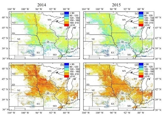
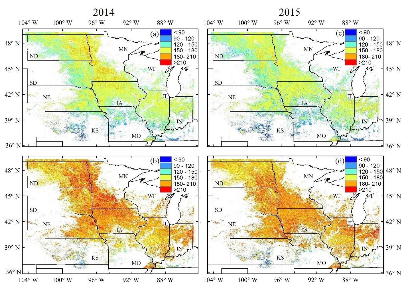
Figure 2 presents spatial patterns in real-time monitoring of crop phenology in 2014 and 2015 over the Midwestern United States. Mid-greenup phase (DOY, day of year) occurred in April and May in Kansas and Missouri and June in Nebraska, Iowa and Illinois. It reached northern areas in North Dakota and Minnesota in July (Figure 2a). Relatively, mid-greenup phase in North Dakota, Minnesota, Iowa and Nebraska occurred up to one month later in 2014 than 2015, indicating substantial interannual variation (Figure 2a,c). As expected, maximum greenness onset (DOY) was delayed with increasing latitudes in both years, ranging from 80 in Kansas and Missouri to 200 in the North Dakota and Minnesota (Figure 2b,d). It is worth noting that spring phenology of crop showed a clear longitudinal pattern from west to east. For example, Minnesota showed a later spring phenology in both 2014 and 2015 compared to similar latitudes in South Dakota.
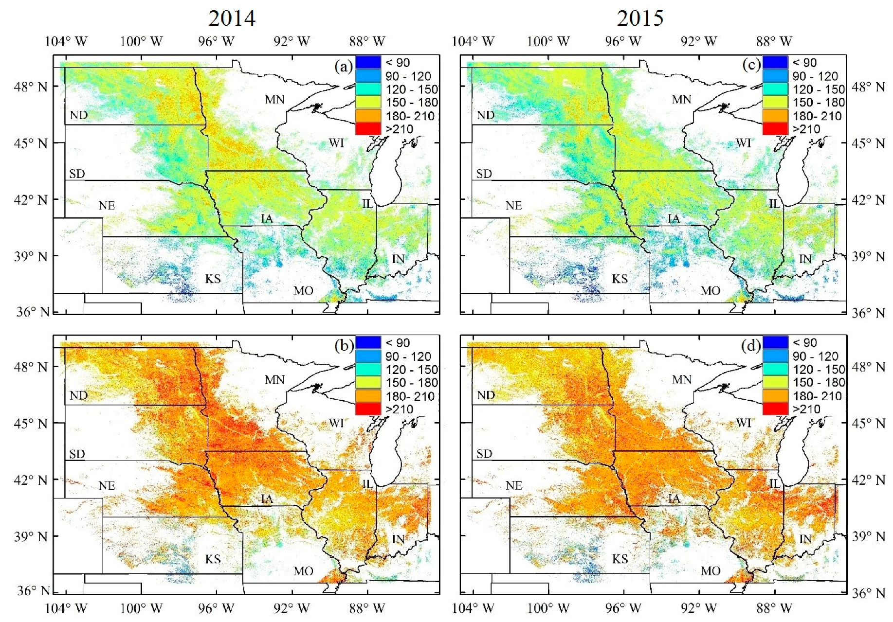
Figure 3 shows the spatial variation in uncertainty of real-time monitoring. Uncertainty was generally <2 days in most crop regions for both mid-greenup phase and maximum greenness onset. It is worth noting that uncertainty was up to 8 days in the western North Dakota and South Dakota for mid-greenup phase in both 2014 and 2015 (Figure 3a,c). However, it decreased to about 4 days for maximum greenness onset because of increasing available VIIRS observations (Figure 3b,d). Moreover, uncertainty was relatively stable along both latitudinal and longitudinal directions across the entire study area in both 2014 and 2015.
3.2. Comparison of VIIRS Vegetation Progress with NASS Crop Progress
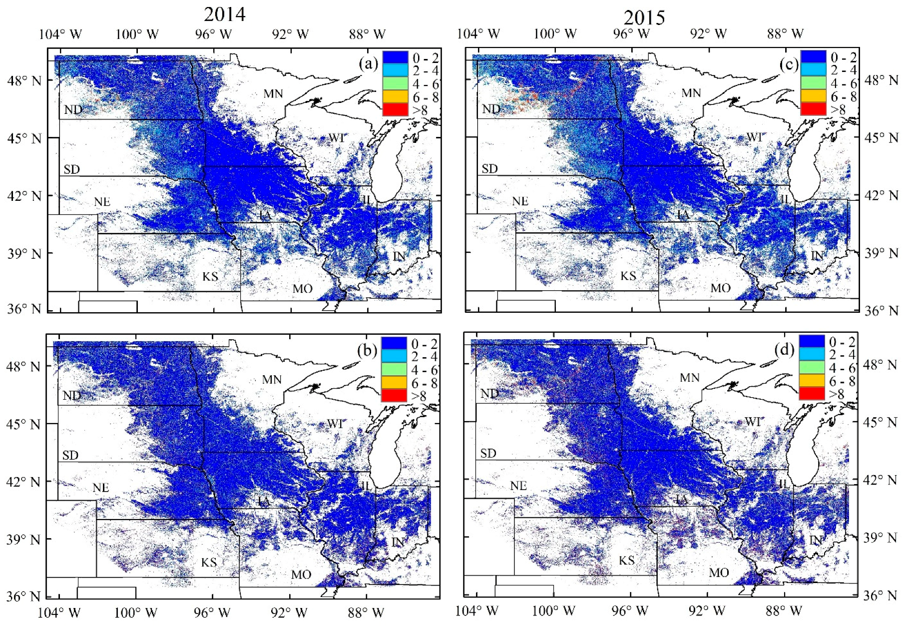
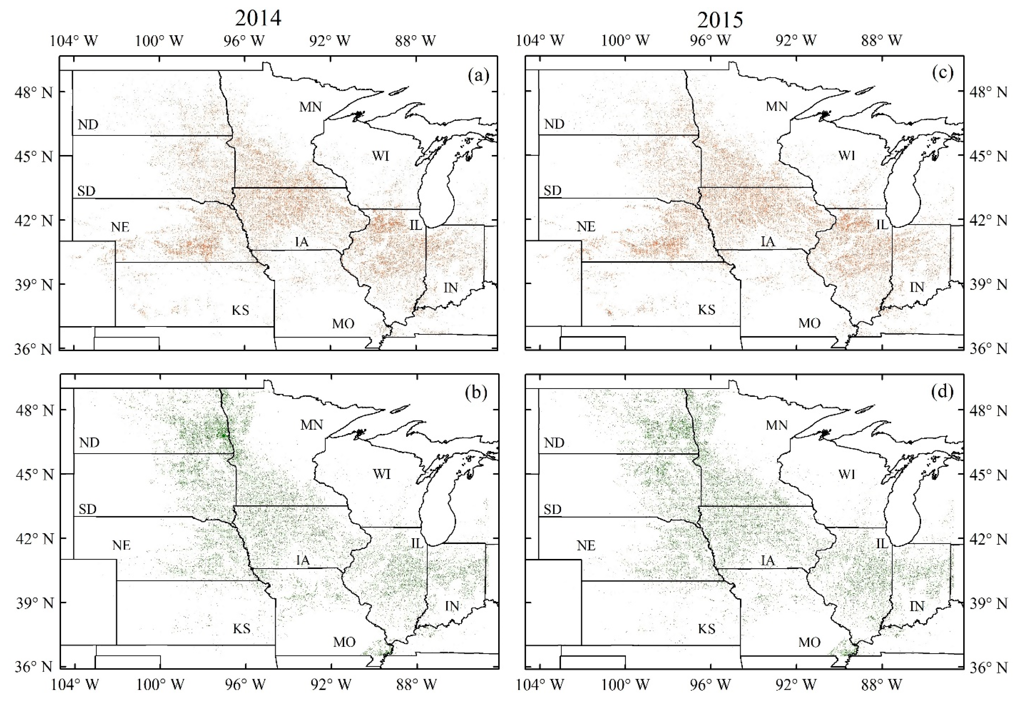
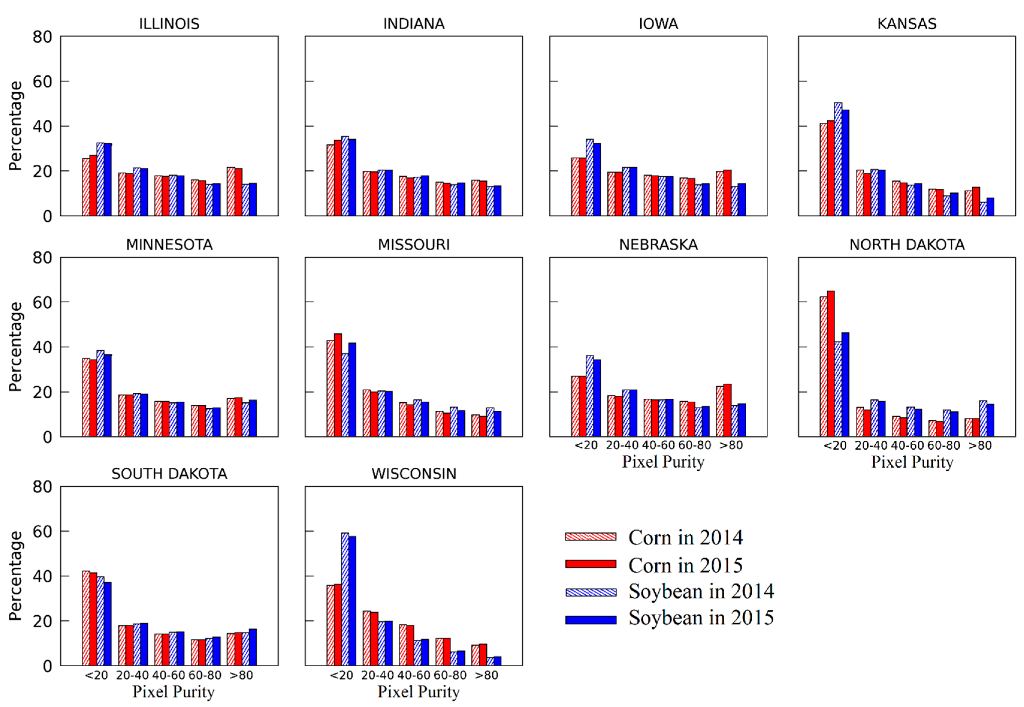
Figure 4 shows spatial patterns of “pure” VIIRS pixels of corn and soybean in 2014 and 2015. The largest area of ‘pure’ corn was found in Iowa, followed by Illinois and Nebraska (Figure 4a,c). The area of ‘pure’ soybean was similarly large in Iowa, Minnesota and North Dakota, followed by Illinois and South Dakota (Figure 4b,d). The histogram shows that the area of ‘pure’ corn (>80%) in most states are larger than that of soybean except for North Dakota, South Dakota and Missouri (Figure 5). Moreover, the percentage of ‘pure’ pixels of corn and soybean was less than 30% for each state. Overall, the spatial pattern and histogram distribution of ‘pure’ corn and soybean in 2015 were similar to those in 2014 (Figure 4 and Figure 5).
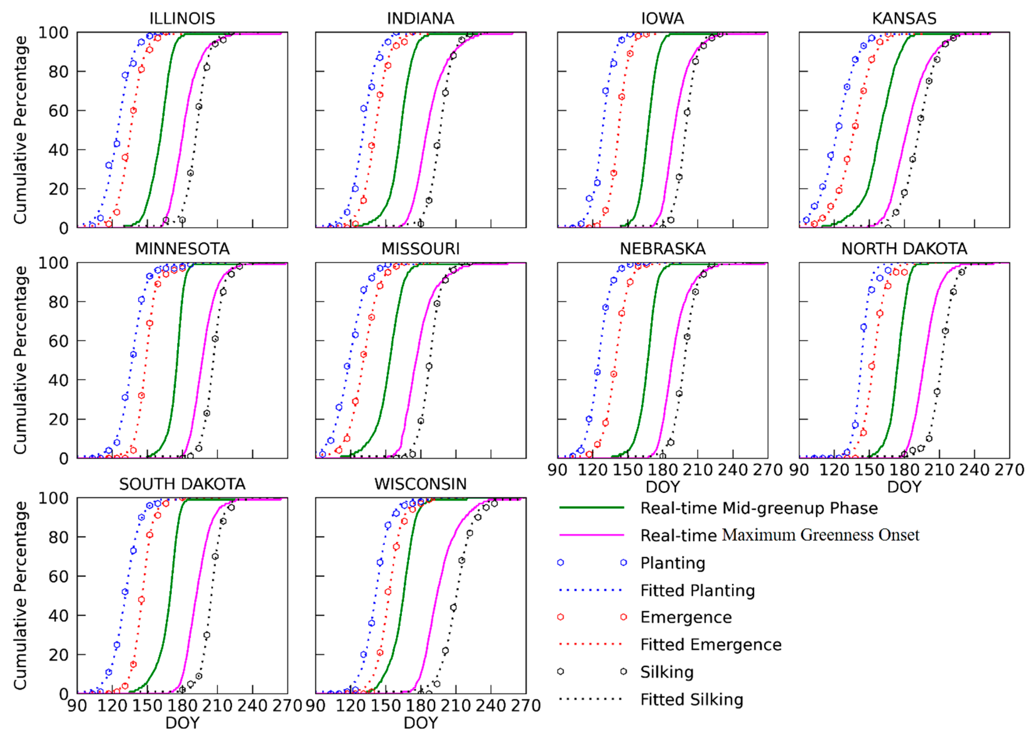
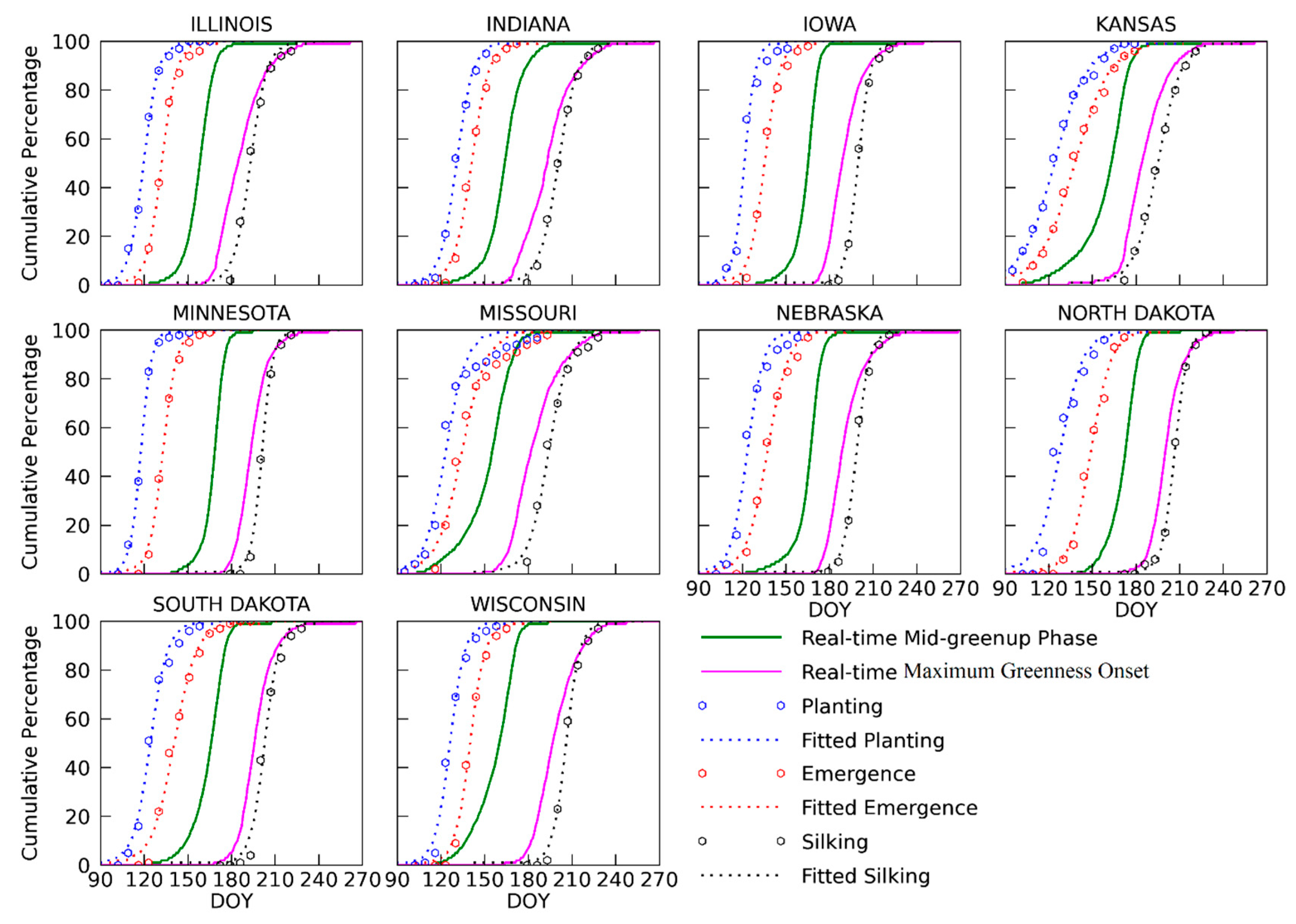
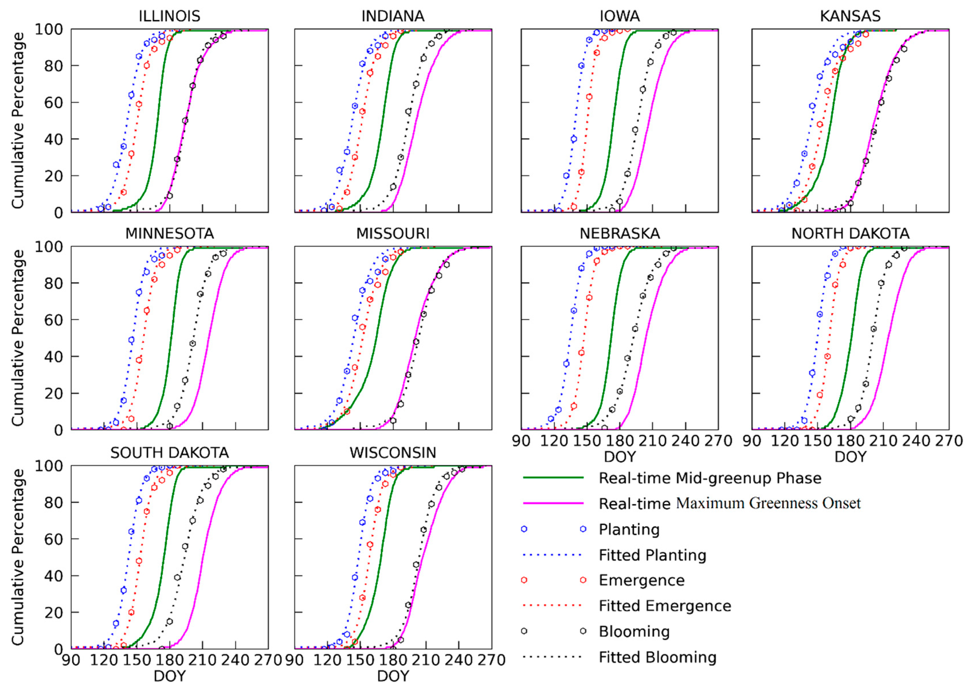
Figure 6 shows the progress of cumulative percent area in spring phenological dates from VIIRS (VIIRS vegetation progress) in comparison with the progress of growth stages reported by USDA NASS for corn in 10 states in 2014. The similar pattern of crop progress was also found in 2015 (Figure 7). The VIIRS vegetation progress in mid-greenup phase was strongly correlated to the NASS CP in planting and emergence dates for corn (R2 ranging from 0.59 to 0.94, p < 0.01) (Table 2). Although the mid-greenup phase from VIIRS was later than the planting and emergence dates from NASS for corn, as expected, their difference of days was consistent with a standard deviation less than 4 days in most states. The mean systematic differences between the mid-greenup phase dates and the planting dates of corn at different areal percentage levels (from 10 to 90% with a 10% interval) in both 2014 and 2015 varied among states ranging from 27 to 44 days with an average of 37 days across all states (Table 2). Similarly, the mean systematic differences between mid-greenup phase and emergence dates ranged from 15 to 31 days with an average of 24 days across all states.
The VIIRS vegetation progress in maximum greenness onset showed a good agreement with the CP in the silking dates across all states in both 2014 and 2015 (Figure 6 and Figure 7). The coefficients of determination (R2) ranged from 0.8 to 1.00 (p < 0.01, Table 2). It is worth noting that maximum greenness onset dates from VIIRS were 8–11 days ahead of the silking dates of corn from NASS with a standard deviation of less than 5 days (Table 2).
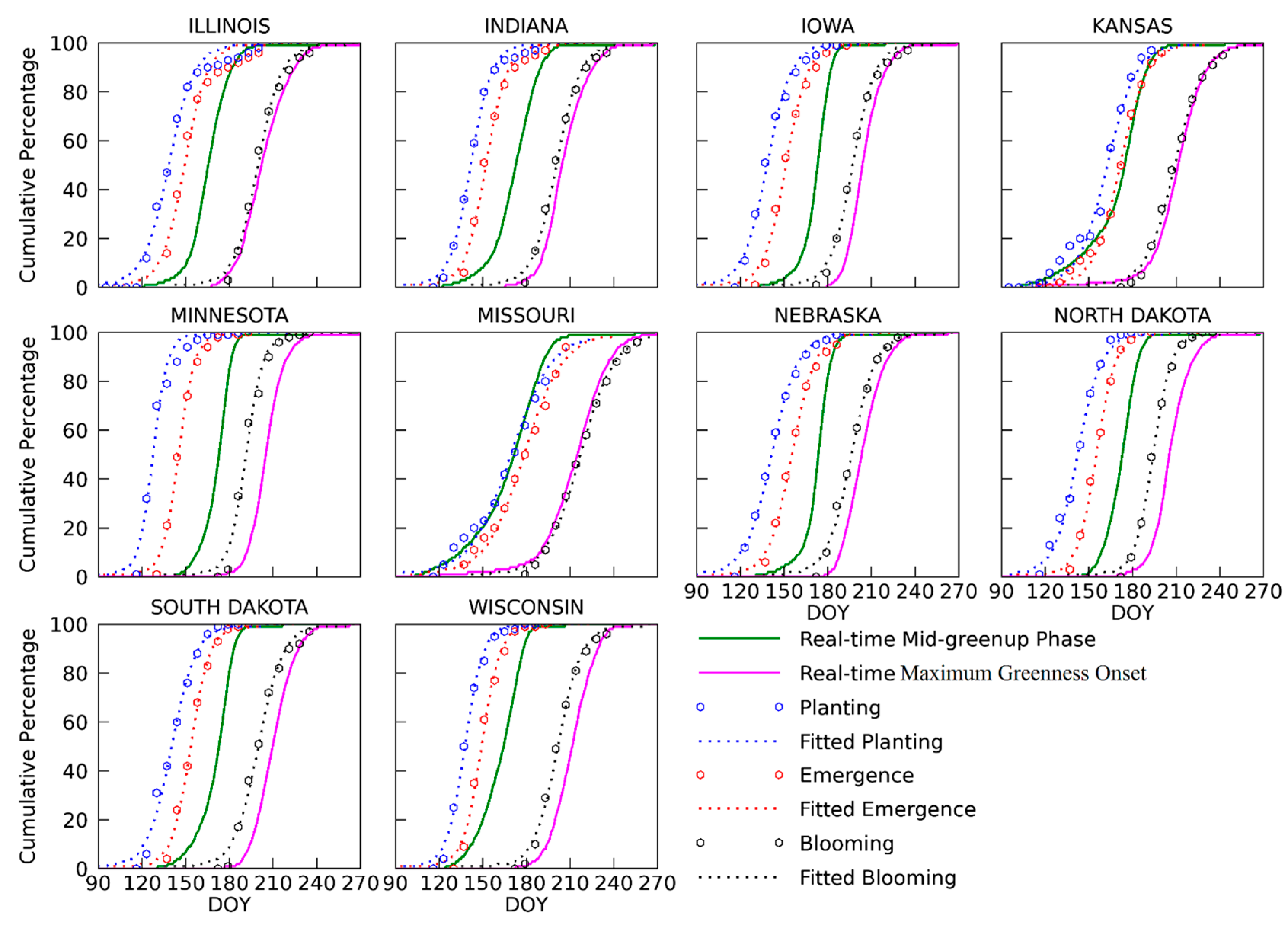
Figure 8 and Figure 9 present the comparison between VIIRS vegetation progress and the NASS crop progress of soybean in 10 states in 2014 and 2015. The VIIRS vegetation progress in mid-greenup phase closely tracked the NASS CP in planting and emergence dates in both 2014 and 2015. The coefficients of determination (R2) ranged from 0.36 to 0.93 (p < 0.01, Table 3). The mean systematic difference between the mid-greenup phase and the planting dates in both 2014 and 2015 ranged from about 22 to 39 days in most states except for Missouri and Kansas (Table 3). The difference was smaller between the mid-greenup phase and emergence dates, which ranged from 12 to 26 days except for Missouri and Kansas. Moreover, the standard deviation of differences between mid-greenup phase and emergence dates was smaller than that between mid-greenup phase and planting dates in most states. The largest standard deviation (about 10 days) was found in Missouri due to substantial interannual variation in systematic differences between 2014 and 2015. Overall, the average of difference across all states between mid-greenup phase and planting dates and between mid-greenup phase and emergence dates was 27 and 16 days, respectively.
The real-time monitoring of maximum greenness onset was consistently later than the blooming dates from CP reports in most states although exceptions were found in Illinois, Kansas and Missouri where VIIRS vegetation progress in maximum greenness onset was almost the same as the NASS CP in blooming dates during the entire greenup phase (R2 0.83 to 0.98, p < 0.01). Their mean systematic differences ranged from 1 to 14 days with a standard deviation of less than 4 days except for Missouri (Table 3). The average of difference across all states was 7 days.
4. Discussion
This study demonstrated that real-time monitoring of crop phenology is feasible using operational VIIRS observations. Comparing VIIRS vegetation progress with NASS crop progress showed they were significantly correlated in both corn and soybean in the Midwestern United States. In particular, VIIRS vegetation progress in mid-greenup phase was significantly correlated to the NASS CP in planting and emergence dates. The result was similar to the previous findings [2] that remotely sensed greenup was strongly correlated with the field reported emergence dates. VIIRS vegetation progress in maximum greenness onset closely tracked the CP in silking dates for corn [2,54] and the CP in blooming dates for soybean. These results suggest that real-time monitoring of crop phenology from VIIRS observations is an effective tool in tracing the crop progress across regional areas.
Theoretically, VIIRS greenup onset should correspond to crop emergences (or turning green) while mid-greenup phase should be located at the middle day between crop emergences and blooming or silking timing [2]. Practically, mid-greenup phase provides a better indictor than greenup onset for monitoring crop emergences in real time. This is associated with the challenge in monitoring greenup onset accurately in real time. During the period around the crop emergence, there are very limited VIIRS observations reflecting crop signal that could be weaker than noise and the VIIRS observations could also be contaminated by clouds. As a result, the accuracy of real-time greenup onset monitoring is relatively low because of the lack of sufficient timely available VIIRS observations with good quality [35]. At the time of real-time monitoring of mid-greenup phase, more satellite observations are accumulated, and the simulated temporal trajectories could well describe the actual crop growth. Moreover, the mid-greenup phase is relatively stable and closely related to crop planting and emergence dates. Therefore, the mid-greenup phase is considered as an effective indicator to backcast the progress of planting and emergence dates.
The maximum greenness onset from satellite observations is close to the date of silking for corn [2]. The silking date is the first reproductive stage and has serious effects on yield [54]. For soybean, similarly, we also chose the first reproductive stage (blooming date) to evaluate the maximum greenness onset. Although soybean could continue to grow for a certain time period after the reproductive stage starts, blooming timing represents most nodes on the main stem with fully developed leaves.
VIIRS vegetation progress is not exactly the same as the field-based NASS CP. Instead of quantifying an absolute accuracy of VIIRS vegetation progress, the comparison between VIIRS vegetation progress and USDA NASS statistics could be used to establish their relationships for the estimation of crop progress from VIIRS phenology. Their consistent differences provide us a promising and useful tool to trace the crop progress in the field. The analyses in this study revealed that the mid-greenup phase date was 27–44 days later than planting dates and 15–31 days later than emergence dates of corn across various states. Similar pattern was found in soybean although the latency was slightly short. These large systematic differences primarily resulted from the different definitions of key phenology stages between field observations and satellite data. Specifically, emergence dates were recorded in NASS data once the crop leaves were first visible, but this early stage was not detectable from satellite observations. According to Zhang et al. [15], greenup onset in a pixel becomes detectable when early leaf emergence occurs in about 30% of the pixel coverage. Similarly, Gao et al. [2] also found that greenup signal lags actual planting and emergence dates about 1–3 weeks. Moreover, the timing of mid-greenup phase is much later than the event of greenup onset. Thus, mid-greenup phase used in this study is theoretically of large latency relative to NASS crop emergence. Besides, the variation in latency of VIIRS phenology monitoring across states was likely associated with the differences of crop growth condition such as soil moisture and temperature and impact factors related to crop management such as fertilizer, irrigation and herbicides [39]. The latency did not show a clear latitudinal gradient, suggesting that the proposed methodology was stable and robust across the different states. However, the standard deviation of difference between VIIRS vegetation progress and NASS CP indicated that latency within a state was almost stable. This suggests that crop progress in planting and emergence dates for corn and soybean could be appropriately backcasted using VIIRS mid-greenup phase from real-time monitoring algorithm by incorporating the lag factor estimated in this study for each state, which agrees with the result that remotely sensed greenup can be effectively applied to backcast emergence dates [2]. Furthermore, the VIIRS-based maximum greenness onset was about 9 days earlier than corn silking dates and 7 days later than soybean blooming dates. This implies that maximum greenness onset is a robust indicator of corn silking and soybean blooming.
More importantly, VIIRS real-time phenology allows us to extract crop development and phenological metrics at each 500 m pixel, which could be applied for improving crop yield prediction at a large scale. It is because numerous previous studies demonstrated that the capability of using 500 m or even much coarser satellite datasets for the estimation of crop yield [5,6,16,55,56,57]. The early and reliable crop yield information is particular important for international humanitarian agencies to organize emergency response and food aid interventions [58]. On the other hand, satellite based phenological metrics could provide information about growth variability in crop fields and thus support agricultural management. This is because the spatial trend of maximum greenness is significantly associated with the management zone pattern [59].
The real-time monitoring capability of crop progress could vary with crop types. The accuracy of real-time monitoring of crop phenology for corn was slightly higher than that for soybean. This is due to the fact that: (1) greenup onset in soybean is later than in corn, which may result in more background vegetation influences in soybean fields; (2) the smaller area of ‘pure’ soybean compared to corn in most states may lead to more soybean pixels containing mixed vegetation types. The results suggest that smaller pixel size may be needed for improving the accuracy of monitoring crop progress in individual species. The estimates of the climatology for corn and soybean phenology may help produce higher accuracy phenology predictions, which requires high spatial resolution satellite observations. For smaller crop fields, it is needed to extend the real-time approach to the medium resolutions sensors such as Landsat 8 and Sentinel-2 [2,15].
Finally, it should be noted that this study was to verify the capability of monitoring crop progress in real time. For the operational purpose of real-time monitoring, the crop type in a given year is required, which is currently not timely available. One potential approach is to employ CDL data in the preceding year at early stage of real-time monitoring because a large amount of crop fields of corn and soybean in the current year remain same as the preceding year. As the number of timely available VIIRS observations increase, it is possible to produce a crop type mask with high accuracy based on the difference between corn and soybean phenology because the planting and emergence dates of corn are always earlier than those of soybean [39]. The crop type data will be replaced for real-time monitoring once the early version of CDL data, which is usually produced in July for NASS internal use, is available. In the near future, we plan to investigate the capability of producing crop type mask from timely available VIIRS observations using the difference between corn and soybean phenology.
5. Conclusions
This study demonstrates for the first time that crop phenology can be monitored in real time by combining climatological phenology and timely available VIIRS data that are operational produced in NOAA. The result shows that VIIRS phenology is promising in tracing crop progress in both corn and soybean in each state, which also provide spatially distributed crop development at a 500 m pixel. Specifically, the detected occurrences of mid-greenup phase in real time is significantly correlated to crop planting dates and emergence dates for both corn and soybean with a consistent lag. Thus, the timing of VIIRS mid-greenup phase could be applied to appropriately backcast the crop planting date and emergence date in individual pixels, which are important parameters in estimating crop yield. Further, the timing of maximum greenness onset is able to predict the corn silking date with an advance of 9 days and the soybean blooming date with a lag of 7 days. Silking or blooming date is the first reproductive stage and critical for monitoring crop yield. These findings demonstrate the capability of VIIRS observations for effectively monitoring temporal dynamics of crop progress in real time at a regional scale. The implementation of monitoring crop phenology in real time during 2014 and 2015 across the Midwestern United States suggests that the developed algorithm is robust and consistent, which can be used for operationally monitoring temporal dynamics of crop progress in real time at a regional scale if the crop type could be obtained timely. The operational implementation of this algorithm could provide significant and timely information for agricultural management and crop yield estimates, which are critical for food security measurements.
Author Contributions
All authors made significant contributions to the work. Specific contributions include research design (X.Z., L.L.), data collection and analysis (L.L.), and manuscript preparation (L.L., X.Z., F.G., Z.Y., Y.Y.), funding acquisition (X.Z., Y.Y.).
Funding
This research was funded by NASA contract NNX15AB96A and NOAA contract JPSS_PGRR2_14/NA14NES4320003.
Acknowledgments
Authors would like to thanks NASA for providing long-term MODIS Nadir BRDF-Adjusted Reflectance (NBAR) data, NOAA for near real time VIIRS data; USDA for the crop progress reports.
Conflicts of Interest
The authors declare no conflict of interest.
References
- Hodges, T. Predicting Crop Phenology; CRC Press: Boca Raton, FL, USA, 1990. [Google Scholar]
- Gao, F.; Anderson, M.C.; Zhang, X.; Yang, Z.; Alfieri, J.G.; Kustas, W.P.; Mueller, R.; Johnson, D.M.; Prueger, J.H. Toward mapping crop progress at field scales through fusion of landsat and modis imagery. Remote Sens. Environ. 2017, 188, 9–25. [Google Scholar] [CrossRef]
- Dingkuhn, M.; Le Gal, P.-Y. Effect of drainage date on yield and dry matter partitioning in irrigated rice. Field Crop. Res. 1996, 46, 117–126. [Google Scholar] [CrossRef]
- Albano, R.; Manfreda, S.; Celano, G. My sirr: Minimalist agro-hydrological model for sustainable irrigation management—Soil moisture and crop dynamics. SoftwareX 2017, 6, 107–117. [Google Scholar] [CrossRef]
- Bolton, D.K.; Friedl, M.A. Forecasting crop yield using remotely sensed vegetation indices and crop phenology metrics. Agric. For. Meteorol. 2013, 173, 74–84. [Google Scholar] [CrossRef]
- Sakamoto, T.; Gitelson, A.A.; Arkebauer, T.J. Modis-based corn grain yield estimation model incorporating crop phenology information. Remote Sens. Environ. 2013, 131, 215–231. [Google Scholar] [CrossRef]
- Zhang, J.; Feng, L.; Yao, F. Improved maize cultivated area estimation over a large scale combining modis—Evi time series data and crop phenological information. ISPRS J. Photogramm. Remote Sens. 2014, 94, 102–113. [Google Scholar] [CrossRef]
- Qiu, B.; Luo, Y.; Tang, Z.; Chen, C.; Lu, D.; Huang, H.; Chen, Y.; Chen, N.; Xu, W. Winter wheat mapping combining variations before and after estimated heading dates. ISPRS J. Photogramm. Remote Sens. 2017, 123, 35–46. [Google Scholar] [CrossRef]
- Gesch, R.W.; Archer, D.W. Influence of sowing date on emergence characteristics of maize seed coated with a temperature-activated polymer. Agron. J. 2005, 97, 1543–1550. [Google Scholar] [CrossRef]
- Liu, L.; Liang, L.; Schwartz, M.D.; Donnelly, A.; Wang, Z.; Schaaf, C.B.; Liu, L. Evaluating the potential of modis satellite data to track temporal dynamics of autumn phenology in a temperate mixed forest. Remote Sens. Environ. 2015, 160, 156–165. [Google Scholar] [CrossRef]
- Setiyono, T.D.; Weiss, A.; Specht, J.; Bastidas, A.M.; Cassman, K.G.; Dobermann, A. Understanding and modeling the effect of temperature and daylength on soybean phenology under high-yield conditions. Field Crop. Res. 2007, 100, 257–271. [Google Scholar] [CrossRef] [Green Version]
- Slafer, G.; Savin, R. Developmental base temperature in different phenological phases of wheat (Triticum aestivum). J. Exp. Bot. 1991, 42, 1077–1082. [Google Scholar] [CrossRef]
- Boschetti, M.; Stroppiana, D.; Brivio, P.A.; Bocchi, S. Multi-year monitoring of rice crop phenology through time series analysis of modis images. Int. J. Remote Sens. 2009, 30, 4643–4662. [Google Scholar] [CrossRef]
- Yang, G.; Liu, J.; Zhao, C.; Li, Z.; Huang, Y.; Yu, H.; Xu, B.; Yang, X.; Zhu, D.; Zhang, X.; et al. Unmanned aerial vehicle remote sensing for field-based crop phenotyping: Current status and perspectives. Front. Plant Sci. 2017, 8, 1111. [Google Scholar] [CrossRef] [PubMed]
- Zhang, X.; Wang, J.; Gao, F.; Liu, Y.; Schaaf, C.; Friedl, M.; Yu, Y.; Jayavelu, S.; Gray, J.; Liu, L.; et al. Exploration of scaling effects on coarse resolution land surface phenology. Remote Sens. Environ. 2017, 190, 318–330. [Google Scholar] [CrossRef]
- Zhang, X.; Zhang, Q. Monitoring interannual variation in global crop yield using long-term avhrr and modis observations. ISPRS J. Photogramm. Remote Sens. 2016, 114, 191–205. [Google Scholar] [CrossRef]
- Sehgal, V.K.; Jain, S.; Aggarwal, P.K.; Jha, S. Deriving crop phenology metrics and their trends using times series NOAA-AVHRR NDVI data. J. Indian Soc. Remote Sens. 2011, 39, 373–381. [Google Scholar] [CrossRef]
- Liu, L.; Zhang, X.; Yu, Y.; Donnelly, A. Detecting spatiotemporal changes of peak foliage coloration in deciduous and mixedforests across the central and eastern united states. Environ. Res. Lett. 2017, 12, 024013. [Google Scholar] [CrossRef]
- Yan, D.; Zhang, X.; Yu, Y.; Guo, W. A comparison of tropical rainforest phenology retrieved from geostationary (SEVIRI) and polar-orbiting (MODIS) sensors across the congo basin. IEEE Trans. Geosci. Remote Sens. 2016, 54, 4867–4881. [Google Scholar] [CrossRef]
- Xin, J.; Yu, Z.; van Leeuwen, L.; Driessen, P.M. Mapping crop key phenological stages in the north china plain using noaa time series images. Int. J. Appl. Earth Obs. Geoinf. 2002, 4, 109–117. [Google Scholar] [CrossRef]
- NASS CPR. 2017. Available online: http://www.nass.usda.gov/Publications/National_Crop_Progress/ (accessed on 1 December 2017).
- Lehecka, G.V. The value of USDA crop progress and condition information: Reactions of corn and soybean futures markets. J. Agric. Resour. Econ. 2014, 39, 88–105. [Google Scholar]
- Daughtry, C.; Cochran, J.; Hollinger, S. Estimating silking and maturity dates of corn for large areas. Agron. J. 1984, 76, 415–420. [Google Scholar] [CrossRef]
- Baker, J.T.; Reddy, V.R. Temperature effects on phenological development and yield of muskmelon. Ann. Bot. 2001, 87, 605–613. [Google Scholar] [CrossRef]
- Hunt, E.R.; Hively, W.D.; Fujikawa, J.S.; Linden, S.D.; Daughtry, T.C.S.; McCarty, W.G. Acquisition of NIR-green-blue digital photographs from unmanned aircraft for crop monitoring. Remote Sens. 2010, 2, 290–305. [Google Scholar] [CrossRef]
- Lelong, C.C.; Burger, P.; Jubelin, G.; Roux, B.; Labbé, S.; Baret, F. Assessment of unmanned aerial vehicles imagery for quantitative monitoring of wheat crop in small plots. Sensors 2008, 8, 3557–3585. [Google Scholar] [CrossRef] [PubMed]
- Liu, Z.; Wu, C.; Liu, Y.; Wang, X.; Fang, B.; Yuan, W.; Ge, Q. Spring green-up date derived from gimms3g and spot-vgt ndvi of winter wheat cropland in the north china plain. ISPRS J. Photogramm. Remote Sens. 2017, 130, 81–91. [Google Scholar] [CrossRef]
- Sakamoto, T.; Wardlow, B.D.; Gitelson, A. Detecting spatiotemporal changes of corn developmental stages in the us corn belt using modis wdrvi data. IEEE Trans. Geosci. Remote Sens. 2011, 49, 1926–1936. [Google Scholar] [CrossRef]
- Sakamoto, T.; Wardlow, B.D.; Gitelson, A.A.; Verma, S.B.; Suyker, A.E.; Arkebauer, T.J. A two-step filtering approach for detecting maize and soybean phenology with time-series modis data. Remote Sens. Environ. 2010, 114, 2146–2159. [Google Scholar] [CrossRef]
- Zeng, L.; Wardlow, B.D.; Wang, R.; Shan, J.; Tadesse, T.; Hayes, M.J.; Li, D. A hybrid approach for detecting corn and soybean phenology with time-series modis data. Remote Sens. Environ. 2016, 181, 237–250. [Google Scholar] [CrossRef]
- Lopez-Sanchez, J.M.; Cloude, S.R.; Ballester-Berman, J.D. Rice phenology monitoring by means of sar polarimetry at x-band. IEEE Trans. Geosci. Remote 2012, 50, 2695–2709. [Google Scholar] [CrossRef]
- Yuzugullu, O.; Marelli, S.; Erten, E.; Sudret, B.; Hajnsek, I. Determining rice growth stage with x-band sar: A metamodel based inversion. Remote Sens. 2017, 9, 460. [Google Scholar] [CrossRef]
- Lokupitiya, E.; Denning, S.; Paustian, K.; Baker, I.; Schaefer, K.; Verma, S.; Meyers, T.; Bernacchi, C.; Suyker, A.; Fischer, M. Incorporation of crop phenology in simple biosphere model (sibcrop) to improve land-atmosphere carbon exchanges from croplands. Biogeosciences 2009, 6, 969–986. [Google Scholar] [CrossRef]
- Cao, C.; Xiong, J.; Blonski, S.; Liu, Q.; Uprety, S.; Shao, X.; Bai, Y.; Weng, F. Suomi npp viirs sensor data record verification, validation, and long-term performance monitoring. J. Geophys. Res. Atmos. 2013, 118, 11664–11678. [Google Scholar] [CrossRef]
- Liu, L.; Zhang, X.; Yu, Y.; Guo, W. Real-time and short-term predictions of spring phenology in north america from viirs data. Remote Sens. Environ. 2017, 194, 89–99. [Google Scholar] [CrossRef]
- Zhang, X.; Goldberg, M.D.; Yu, Y. Prototype for monitoring and forecasting fall foliage coloration in real time from satellite data. Agric. For. Meteorol. 2012, 158–159, 21–29. [Google Scholar] [CrossRef]
- Twine, T.E.; Kucharik, C.J. Climate impacts on net primary productivity trends in natural and managed ecosystems of the central and eastern united states. Agric. For. Meteorol. 2009, 149, 2143–2161. [Google Scholar] [CrossRef]
- Zhong, L.; Gong, P.; Biging, G.S. Efficient corn and soybean mapping with temporal extendability: A multi-year experiment using landsat imagery. Remote Sens. Environ. 2014, 140, 1–13. [Google Scholar] [CrossRef]
- Sacks, W.J.; Kucharik, C.J. Crop management and phenology trends in the u.S. Corn belt: Impacts on yields, evapotranspiration and energy balance. Agric. For. Meteorol. 2011, 151, 882–894. [Google Scholar] [CrossRef]
- Bastidas, A.M.; Setiyono, T.D.; Dobermann, A.; Cassman, K.G.; Elmore, R.W.; Graef, G.L.; Specht, J.E. Soybean sowing date: The vegetative, reproductive, and agronomic impacts. Crop Sci. 2008, 48, 727–740. [Google Scholar] [CrossRef]
- Twine, T.E.; Kucharik, C.J.; Foley, J.A. Effects of land cover change on the energy and water balance of the mississippi river basin. J. Hydrometeorol. 2004, 5, 640–655. [Google Scholar] [CrossRef]
- Jiang, Z.; Huete, A.R.; Didan, K.; Miura, T. Development of a two-band enhanced vegetation index without a blue band. Remote Sens. Environ. 2008, 112, 3833–3845. [Google Scholar] [CrossRef]
- Zhang, X. Reconstruction of a complete global time series of daily vegetation index trajectory from long-term avhrr data. Remote Sens. Environ. 2015, 156, 457–472. [Google Scholar] [CrossRef]
- Ratkowsky, D.A. Nonlinear Regression Modeling: A Unified Practical Approach. Statistics: Textbooks and Monographs; Marcel Dekker, Inc.: New York, NY, USA, 1983. [Google Scholar]
- Richards, F.J. A flexible growth function for empirical use. J. Exp. Bot. 1959, 10, 290–301. [Google Scholar] [CrossRef]
- Zhang, X.Y.; Friedl, M.A.; Schaaf, C.B.; Strahler, A.H.; Hodges, J.C.F.; Gao, F.; Reed, B.C.; Huete, A. Monitoring vegetation phenology using modis. Remote Sens. Environ. 2003, 84, 471–475. [Google Scholar] [CrossRef]
- Zhang, X.; Friedl, M.A.; Schaaf, C.B. Global vegetation phenology from moderate resolution imaging spectroradiometer (MODIS): Evaluation of global patterns and comparison with in situ measurements. J. Geophys. Res. 2006, 111, G04017. [Google Scholar] [CrossRef]
- Zhang, X. Land surface phenology: Climate data record and real-time monitoring. In Reference Module in Earth Systems and Environmental Sciences; Elsevier: New York, NY, USA, 2018. [Google Scholar]
- Vargas, M.; Miura, T.; Shabanov, N.; Kato, A. An initial assessment of suomi npp viirs vegetation index edr. J. Geophys. Res. Atmos. 2013, 118, 12301–12316. [Google Scholar] [CrossRef]
- Zhang, X.; Liu, L.; Yan, D. Comparisons of global land surface seasonality and phenology derived from avhrr, modis, and viirs data. J. Geophys. Res. Biogeosci. 2017, 122, 2017JG003811. [Google Scholar] [CrossRef]
- NASS Terms. Available online: https://www.nass.usda.gov/Publications/National_Crop_Progress/Terms_and_Definitions/index.php (accessed on 1 December 2017).
- Boryan, C.; Yang, Z.; Mueller, R.; Craig, M. Monitoring us agriculture: The us department of agriculture, national agricultural statistics service, cropland data layer program. Geocarto Int. 2011, 26, 341–358. [Google Scholar] [CrossRef]
- Han, W.; Yang, Z.; Di, L.; Mueller, R. Cropscape: A web service based application for exploring and disseminating us conterminous geospatial cropland data products for decision support. Comput. Electron. Agric. 2012, 84, 111–123. [Google Scholar] [CrossRef]
- Gallo, K.; Flesch, T. Large-area crop monitoring with the noaa avhrr: Estimating the silking stage of corn development. Remote Sens. Environ. 1989, 27, 73–80. [Google Scholar] [CrossRef]
- Lee, R.; Kastens, D.; Price, K.; Martinko, E. Forecasting Corn Yield in Iowa Using Remotely Sensed Data and Vegetation Phenology Information. In Proceedings of the Second International Conference on Geospatial Information in Agriculture and Forestry, Lake Buena Vista, FL, USA, 10–12 January 2000; pp. 460–467. [Google Scholar]
- Becker-Reshef, I.; Vermote, E.; Lindeman, M.; Justice, C. A generalized regression-based model for forecasting winter wheat yields in kansas and ukraine using modis data. Remote Sens. Environ. 2010, 114, 1312–1323. [Google Scholar] [CrossRef]
- Kowalik, W.; Dabrowska-Zielinska, K.; Meroni, M.; Raczka, T.U.; de Wit, A. Yield estimation using spot-vegetation products: A case study of wheat in european countries. Int. J. Appl. Earth Obs. Geoinf. 2014, 32, 228–239. [Google Scholar] [CrossRef]
- Rembold, F.; Atzberger, C.; Savin, I.; Rojas, O. Using low resolution satellite imagery for yield prediction and yield anomaly detection. Remote Sens. 2013, 5, 1704–1733. [Google Scholar] [CrossRef] [Green Version]
- Araya, S.; Ostendorf, B.; Lyle, G.; Lewis, M. Remote sensing derived phenological metrics to assess the spatio-temporal growth variability in cropping fields. Adv. Remote Sens. 2017, 6, 212–228. [Google Scholar] [CrossRef]
Figure 1.
The spatial pattern of vegetation types in the study area overlaid with mosaicked MODIS four tiles (h10v04, h10v05, h11v04 and h11v05), state boundaries (black lines) and state abbreviations. IL—Illinois, IN—Indiana, IA—Iowa, KS—Kansas, MN—Minnesota, MO—Missouri, NE—Nebraska, ND—North Dakota, SD—South Dakota, and WI—Wisconsin.

Figure 2.
Spatial patterns in real-time monitoring of crop phenology (DOY, day of year) in the Midwestern United States in 2014 (a,b) and 2015 (c,d). Mid-greenup phase (a,c) and maximum greenness onset (b,d). The state abbreviation is the same as Figure 1.
Figure 2.
Spatial patterns in real-time monitoring of crop phenology (DOY, day of year) in the Midwestern United States in 2014 (a,b) and 2015 (c,d). Mid-greenup phase (a,c) and maximum greenness onset (b,d). The state abbreviation is the same as Figure 1.

Figure 3.
Spatial patterns in uncertainty (standard deviation, days) of real-time monitoring of crop phenology in the Midwestern United States in 2014 (a,b) and 2015 (c,d). Mid-greenup phase (a,c) and maximum greenness onset (b,d). The state abbreviation is the same as Figure 1.
Figure 3.
Spatial patterns in uncertainty (standard deviation, days) of real-time monitoring of crop phenology in the Midwestern United States in 2014 (a,b) and 2015 (c,d). Mid-greenup phase (a,c) and maximum greenness onset (b,d). The state abbreviation is the same as Figure 1.

Figure 4.
Spatial distribution of “pure” VIIRS pixels of corn (a,c) and soybean (b,d) in 2014 and 2015. The state abbreviation is the same as Figure 1.
Figure 4.
Spatial distribution of “pure” VIIRS pixels of corn (a,c) and soybean (b,d) in 2014 and 2015. The state abbreviation is the same as Figure 1.

Figure 5.
The histogram of areal percentages of corn and soybean among all pixels with the same crop type at different purities (<20%, 20–40%, 40–60%, 60–80% and >80%) for each state in 2014 and 2015.
Figure 5.
The histogram of areal percentages of corn and soybean among all pixels with the same crop type at different purities (<20%, 20–40%, 40–60%, 60–80% and >80%) for each state in 2014 and 2015.

Figure 6.
Progress of cumulative percent area in VIIRS mid-greenup phase (solid green lines) and maximum greenness onset (solid magenta lines) and NASS crop progress in planting (dotted blue lines), emergence (dotted red lines) and silking (dotted black lines) for corn at a state level in 2014.
Figure 6.
Progress of cumulative percent area in VIIRS mid-greenup phase (solid green lines) and maximum greenness onset (solid magenta lines) and NASS crop progress in planting (dotted blue lines), emergence (dotted red lines) and silking (dotted black lines) for corn at a state level in 2014.

Figure 7.
Progress of cumulative percent area in VIIRS mid-greenup phase (solid green lines) and maximum greenness onset (solid magenta lines) and NASS crop progress in planting (dotted blue lines), emergence (dotted red lines) and silking (dotted black lines) for corn at a state level in 2015.
Figure 7.
Progress of cumulative percent area in VIIRS mid-greenup phase (solid green lines) and maximum greenness onset (solid magenta lines) and NASS crop progress in planting (dotted blue lines), emergence (dotted red lines) and silking (dotted black lines) for corn at a state level in 2015.

Figure 8.
Progress of cumulative percent area in VIIRS mid-greenup phase (solid blue lines) and maximum greenness onset (solid magenta lines) and NASS crop progress in planting (dotted blue lines), emergence (dotted red lines) and blooming (dotted black lines) for soybean at a state level in 2014.
Figure 8.
Progress of cumulative percent area in VIIRS mid-greenup phase (solid blue lines) and maximum greenness onset (solid magenta lines) and NASS crop progress in planting (dotted blue lines), emergence (dotted red lines) and blooming (dotted black lines) for soybean at a state level in 2014.

Figure 9.
Progress of cumulative percent area in VIIRS mid-greenup phase (solid blue lines) and maximum greenness onset (solid magenta lines) and NASS crop progress in planting (dotted blue lines), emergence (dotted red lines) and blooming (dotted black lines) for soybean at a state level in 2015.
Figure 9.
Progress of cumulative percent area in VIIRS mid-greenup phase (solid blue lines) and maximum greenness onset (solid magenta lines) and NASS crop progress in planting (dotted blue lines), emergence (dotted red lines) and blooming (dotted black lines) for soybean at a state level in 2015.


Table 1.
Key crop growth stages in spring and descriptions for corn and soybean from USDA NASS.
| Corn | Description | Soybean | Description | Phenology from Remote Sensing |
|---|---|---|---|---|
| Planting | A crop is considered planted when the seeds are placed in the ground | Planting | A crop is considered planted when the seeds are placed in the ground | No detection, but correlated to mid-greenup phase |
| Emergence | As soon as the plants are visible | Emergence | As soon as the plants are visible | Greenup onset (or correlated to mid-greenup phase) |
| Silking | The emergence of silk-like strands from the end of ears | Blooming | A plant should be considered as blooming as soon as one bloom appears | Maximum greenness onset |
Table 2.
Parameters of statistical comparison between VIIRS vegetation progress and NASS CP for corn in both 2014 and 2015 for each state. The parameters are mean systematic difference (Mean), standard deviation (SD), regression slope (A), regression intercept (B), and coefficient of determination (R2). The linear regression (p < 0.01) was obtained using VIIRS vegetation progress against NASS CP. The last row shows the average of difference, standard deviation, and R2 across all states.
| State | Planting and Mid-Greenup Phase | Emergence and Mid-Greenup Phase | Silking and Maximum Greenness Onset | |||||||||
|---|---|---|---|---|---|---|---|---|---|---|---|---|
| Mean ± SD | A | B | R2 | Mean ± SD | A | B | R2 | Mean ± SD | A | B | R2 | |
| ND | 38 ± 7.1 | 0.6 | 95.6 | 0.68 | 22 ± 2.1 | 0.7 | 66.2 | 0.93 | −10 ± 4.6 | 1 | −2.4 | 0.86 |
| MN | 44 ± 6.7 | 0.4 | 122.8 | 0.82 | 31 ± 4.9 | 0.5 | 102.1 | 0.84 | −8 ± 2.8 | 1.2 | −53.7 | 0.98 |
| WI | 27 ± 5.5 | 0.9 | 37 | 0.82 | 15 ± 4.4 | 0.9 | 32.8 | 0.81 | −11 ± 5.3 | 1.2 | −52.4 | 0.92 |
| SD | 39 ± 2.7 | 0.8 | 60.7 | 0.85 | 23 ± 2.4 | 1.1 | −1.9 | 0.71 | −9 ± 3.7 | 1.1 | −38.1 | 0.95 |
| NE | 42 ± 1.7 | 1.3 | −4.1 | 0.69 | 28 ± 2.8 | 0.7 | 62.4 | 0.94 | −9 ± 3.3 | 1.4 | −79.2 | 0.98 |
| IA | 41 ± 2.1 | 0.7 | 70.8 | 0.92 | 27 ± 2.2 | 0.9 | 43.9 | 0.89 | −9 ± 3.3 | 1.3 | −74.8 | 1.00 |
| IL | 37 ± 1.5 | 1.5 | −26.7 | 0.81 | 26 ± 0.8 | 1.6 | −50.8 | 0.75 | −9 ± 3.8 | 1.4 | −90.1 | 0.81 |
| IN | 32 ± 1.3 | 1.6 | −52.9 | 0.86 | 22 ± 1.1 | 1.4 | −43.2 | 0.82 | −9 ± 4.6 | 1.5 | −101.8 | 0.99 |
| KS | 37 ± 3.4 | 0.7 | 68.5 | 0.91 | 22 ± 4.1 | 0.9 | 30.6 | 0.88 | −9 ± 2.4 | 1.2 | −43.8 | 0.98 |
| MO | 32 ± 3.5 | 0.7 | 61 | 0.75 | 20 ± 2.5 | 0.7 | 53.7 | 0.59 | −10 ± 3.9 | 1.6 | −117.1 | 0.8 |
| Ave | 37 ± 4 | 0.81 | 24 ± 3 | 0.82 | −9 ± 4 | 0.93 | ||||||
Table 3.
Parameters of statistical comparison between VIIRS vegetation progress and NASS CP for soybean in both 2014 and 2015 for each state. The parameters are mean systematic difference (Mean), standard deviation (SD), regression slope (A), regression intercept (B), and coefficient of determination (R2). The linear regression (p < 0.01) was obtained using VIIRS vegetation progress against NASS CP. The last row shows the average of difference, standard deviation, and R2 across all states.
| State | Planting and Mid-Greenup Phase | Emergence and Mid-Greenup Phase | Blooming and Maximum Greenness Onset | |||||||||
|---|---|---|---|---|---|---|---|---|---|---|---|---|
| Mean ± SD | A | B | R2 | Mean ± SD | A | B | R2 | Mean ± SD | A | B | R2 | |
| ND | 30 ± 2.4 | 1.6 | −56.9 | 0.73 | 18 ± 1.6 | 2 | −139 | 0.76 | 13 ± 2.3 | 1.3 | −43 | 0.95 |
| MN | 39 ± 5.2 | 0.9 | 47 | 0.62 | 26 ± 1.8 | 1 | 16.4 | 0.65 | 14 ± 0.7 | 1.1 | −15.6 | 0.92 |
| WI | 22 ± 3.7 | 1 | 17.6 | 0.91 | 12 ± 3.1 | 1 | 14.2 | 0.91 | 7 ± 3.3 | 1 | 14.4 | 0.96 |
| SD | 31 ± 2.4 | 1.1 | 17.1 | 0.87 | 19 ± 2.1 | 1.1 | −2.1 | 0.82 | 14 ± 4.2 | 0.9 | 36.3 | 0.87 |
| NE | 35 ± 5.4 | 0.9 | 49.7 | 0.36 | 21 ± 4.9 | 1.5 | −47.9 | 0.57 | 10 ± 2.8 | 1 | 7.8 | 0.94 |
| IA | 34 ± 3.5 | 0.8 | 55.4 | 0.45 | 22 ± 3.1 | 1 | 11.4 | 0.59 | 9 ± 2.4 | 0.9 | 24.6 | 0.94 |
| IL | 27 ± 2.7 | 0.6 | 83.6 | 0.85 | 17 ± 1.9 | 0.7 | 60.2 | 0.5 | 2 ± 2.5 | 1 | −2.4 | 0.98 |
| IN | 29 ± 2.5 | 0.9 | 34.9 | 0.86 | 19 ± 2.0 | 0.9 | 33.7 | 0.89 | 7 ± 2.6 | 1.2 | −29.3 | 0.84 |
| KS | 12 ± 5.4 | 1 | 3.1 | 0.93 | 3 ± 5.2 | 1.1 | −13.8 | 0.91 | 1 ± 2.2 | 1.2 | −34.8 | 0.91 |
| MO | 9 ± 10.3 | 0.9 | 29 | 0.83 | 0 ± 10.6 | 0.9 | 17.6 | 0.8 | −2 ± 1.3 | 1.2 | −39.5 | 0.83 |
| Ave | 27 ± 4 | 0.74 | 16 ± 4 | 0.74 | 7 ± 2 | 0.92 | ||||||
© 2018 by the authors. Licensee MDPI, Basel, Switzerland. This article is an open access article distributed under the terms and conditions of the Creative Commons Attribution (CC BY) license (http://creativecommons.org/licenses/by/4.0/).
Share and Cite
MDPI and ACS Style
Liu, L.; Zhang, X.; Yu, Y.; Gao, F.; Yang, Z. Real-Time Monitoring of Crop Phenology in the Midwestern United States Using VIIRS Observations. Remote Sens. 2018, 10, 1540. https://doi.org/10.3390/rs10101540
AMA Style
Liu L, Zhang X, Yu Y, Gao F, Yang Z. Real-Time Monitoring of Crop Phenology in the Midwestern United States Using VIIRS Observations. Remote Sensing. 2018; 10(10):1540. https://doi.org/10.3390/rs10101540
Chicago/Turabian StyleLiu, Lingling, Xiaoyang Zhang, Yunyue Yu, Feng Gao, and Zhengwei Yang. 2018. "Real-Time Monitoring of Crop Phenology in the Midwestern United States Using VIIRS Observations" Remote Sensing 10, no. 10: 1540. https://doi.org/10.3390/rs10101540
Note that from the first issue of 2016, this journal uses article numbers instead of page numbers. See further details here.