Enhancing Land Cover Mapping through Integration of Pixel-Based and Object-Based Classifications from Remotely Sensed Imagery


1
School of Earth Sciences and Engineering, Hohai University, Nanjing 210098, China
2
State Key Laboratory of Resources and Environmental Information System, Institute of Geographical Sciences and Natural Resources Research, Chinese Academy of Sciences, Beijing 100101, China
3
School of Geography Science, Nanjing Normal University, Nanjing 210023, China
*
Author to whom correspondence should be addressed.
Remote Sens. 2018, 10(1), 77; https://doi.org/10.3390/rs10010077
Submission received: 24 November 2017
/
Revised: 3 January 2018
/
Accepted: 6 January 2018
/
Published: 8 January 2018
(This article belongs to the Special Issue Uncertainty in Remote Sensing Image Analysis)
Abstract
:Pixel-based and object-based classifications are two commonly used approaches in extracting land cover information from remote sensing images. However, they each have their own inherent merits and limitations. This study, therefore, proposes a new classification method through the integration of pixel-based and object-based classifications (IPOC). Firstly, it employs pixel-based soft classification to obtain the class proportions of pixels to characterize the land cover details from pixel-scale properties. Secondly, it adopts area-to-point kriging to explore the class spatial dependence between objects for each pixel from object-based soft classification results. Thirdly, the class proportions of pixels and the class spatial dependence of pixels are fused as the class occurrence of pixels. Last, a linear optimization model on objects is built to determine the optimal class label of pixels within each object. Two remote sensing images are used to evaluate the effectiveness of IPOC. The experimental results demonstrate that IPOC performs better than the traditional pixel-based hard classification and object-based hard classification methods. Specifically, the overall accuracy of IPOC is 7.64% higher than that of pixel-based hard classification and 4.64% greater than that of object-based hard classification in the first experiment, while the overall accuracy improvements in the second experiment are 3.59% and 3.42%, respectively. Meanwhile, IPOC produces less salt and pepper effect than the pixel-based hard classification method and generates more accurate land cover details and small patches than the object-based hard classification method.
1. Introduction
Land cover is a fundamental variable in many scientific studies such as resource investigations, global climate change, and sustainable development [1,2,3]. The use of classifications is an efficient way to extract land cover information from remote sensing images [4,5]. Classification approaches can be divided into two general categories: (i) pixel-based classification, and (ii) object-based classification [6,7]. Pixel-based classification approaches use the pixel as the basic analysis unit while object-based classification approaches employ the object (i.e., a group of adjacent pixels) as the basic analysis unit [6]. Pixel-based classification contains mainly two types: (i) pixel-based hard classification, and (ii) pixel-based soft classification (PSC) (also termed as spectral unmixing) [7]. Pixel-based hard classification supposes each pixel is pure and it classifies individual pixels into mutually exclusive land cover classes in terms of their spectral properties. By contrast, PSC produces the proportions (i.e., possibilities of class occurrence) of land cover classes within each pixel because mixed pixels that contain more than one class are inevitable in various remote sensing images [8]. Usually, PSC results can be converted into pixel-based hard classification results by assigning the class label with the maximum proportion to the pixel. Pixel-based classification has long been the mainstay technique for classifying remote sensing images [9,10], especially low/medium spatial resolution remote sensing images (e.g., MODIS images and Landsat images). In recent years, with the advent of high and very-high spatial resolution remote sensing images, the advanced object-based classification has been developed [6]. Object-based classification has two differences from pixel-based classification. The first difference is that object-based classification performs in units of objects derived from image segmentation whereas the process of pixel-based classification is directly based on image pixels. The second difference is that pixel-based classification uses mainly the pixels’ spectral properties while object-based classification employs not only spectral properties of objects but also objects’ spatial, textural, and shape properties [6]. Despite these differences, both pixel-based and object-based classifications have achieved a relatively satisfactory performance in extracting land cover information from different remote sensing images [6,7]; each has their own inherent merits and limitations. Pixel-based classification does not change the spectral properties of the pixels and may preserve land cover details; however, it is difficult to use complementary properties (e.g., spatial structures) [11,12], which may lead to the salt and pepper effect and the unmaintained structure of land cover patches in classified maps [6,13]. Although object-based classification can use both spectral and complementary properties of objects, the spectral properties of objects are smoothed by image segmentation [14]; the segmentation errors caused by under-segmentation and over-segmentation could affect the accuracy of object-based classification results [15]. The smoothed spectral properties of objects may be suitable for heterogeneous land areas. However, they are inappropriate for homogeneous land regions because the spectral separability between different classes are smoothed and reduced in homogeneous areas [6,14], especially for medium spatial resolution remote sensing images. Generating accurate image segmentation results is considered as the crucial process in object-based classification; however, image segmentation errors are often inevitable [6,13,15,16,17]. For instance, image segmentation usually produces the mis-segmented boundary of objects (e.g., the object marked by the red polygon in Figure 1a). Meanwhile, some important small land cover patches cannot be successfully segmented and they are merged into adjacent objects (e.g., the object marked by the red polygon in Figure 1b). Basically, the two marked objects are mixed objects that include more than one land cover class [15,18]. The mixed object in Figure 1a could be regarded as the classic high-resolution type defined by Woodcock and Strahler [19], where the segmented objects are smaller than the objects of interest and they often occur in intersection regions between different large land cover patches. Land cover information in the intersection region of this type of mixed objects is often spatially related with neighboring objects. By contrast, the mixed object in Figure 1b could be viewed as the classic low-resolution type [19,20], where the segmented objects are larger than the objects of interest and they usually involve isolated small land cover patches. In traditional object-based classification, mixed objects have mixed properties of different land cover classes and all pixels within each mixed object have to be assigned to the same class (i.e., a hard classification process on objects), and thus reducing the accuracy of classified maps [15].
To address the aforementioned problems in the object-based classification, several studies have been conducted to combine pixel-based and object-based classifications to improve the accuracy of land cover maps [14,21,22,23,24,25,26,27]. They can be divided into three groups: (i) majority rule; (ii) the best class merging rule; and (iii) expert knowledge. The methods in the group of majority rule first perform pixel-based classification and image segmentation and then they assign an object to a specific class that has the majority number of pixels within the object in pixel-based classified maps [21,22]. The second group of methods first implement both pixel-based and object-based classifications and then the result of each class with the highest accuracy from either the pixel-based or object-based classified map is selected and all selected results are finally merged into a combined classification map [14,24]. The last group of methods mainly builds comprehensive decision rules to assign each object to a particular class according to expert knowledge [23,25,26,27]. Although these methods have achieved improved land cover maps, less attention has been paid to handling the mixed object problem for producing detailed land cover information within a mixed object. Mixed objects are the analog of mixed pixels. In the pixel-based classification, the super-resolution mapping (SRM) technique was developed as a post-processing step of PSC to deal with the land cover spatial distribution uncertainty of mixed pixels. SRM can determine where different classes spatially distribute within a mixed pixel [20,28,29,30,31,32,33,34,35,36,37,38,39,40]. Unfortunately, no research such as SRM for mixed objects has been proposed for handling the land cover spatial distribution uncertainty of mixed objects by estimating the accurate spatial distribution of different classes within mixed objects at the pixel scale.
The purpose of this study is to propose a novel classification method through the integration of pixel-based and object-based classifications (IPOC). It aims to estimate where different land cover classes spatially distribute within mixed objects in traditional remote sensing image classifications. IPOC uses the basic idea of SRM to deal with the mixed object uncertainty problem by taking advantage of both pixel-based and object-based classifications. The class proportions of pixels generated by PSC are used to represent land cover details pixel by pixel, especially the small land cover patches in low-resolution mixed objects (e.g., the low-resolution mixed object in Figure 1b). The class spatial relationships are explored from object-based soft classification (OSC) results for each pixel to characterize the class spatial dependence between objects because some mis-segmented land cover patches in the intersection regions (e.g., the high-resolution type mixed object in Figure 1a) are usually spatially dependent on neighboring objects. The class proportions of pixels and the class spatial dependence of pixels are further fused to determine the optimal class labels of pixels within each object. Two experiments are conducted to assess the effectiveness of IPOC.
2. Methods
The flowchart of IPOC is presented in Figure 2. With the inputs of remote sensing images and training samples, IPOC involves four main processes: (i) generating the land cover class proportions of each pixel and each object; (ii) estimating the class spatial dependence from object-scale properties for each pixel; (iii) fusing the class proportions and the class spatial dependence of pixels; and (iv) determining the optimal class label of each pixel within an object. More details about the four processes are described below.
2.1. Generating the Class Proportions of Pixels and Objects
Pixel-based classification is able to represent land cover details pixel by pixel according to unsmoothed spectral properties. Object-based classification not only uses the spectral properties of objects but also considers objects’ complementary properties, such as spatial structures. Therefore, they are involved in IPOC to make full use of pixel-based and object-based classifications. Both PSC and OSC results can provide the class proportions (between 0 and 1) of the analysis units (i.e., pixel and object) to describe how much area of each class the unit contains. IPOC uses the PSC to generate the class proportions of pixels, which facilitates in characterizing the land cover details for each pixel. The OSC is involved in IPOC to use spectral and complementary properties of objects and produces the class proportions for each object. It is noteworthy that both PSC and OSC can generate the class proportions of each analysis unit by a soft classifier (e.g., a soft support vector machine classifier).
2.2. Estimating the Class Spatial Dependence from Object-Scale Properties for Each Pixel
Although PSC results provide the class proportions pixel by pixel, OSC results cannot specify the pixels’ class proportions using object-scale properties. Meanwhile, the class proportions of pixels generated only by PSC cannot use object-scale spectral and complementary properties. Furthermore, the class spatial relationships (i.e., dependence) between objects shown in Figure 1 fail to use pixel by pixel in PSC. Therefore, in order to consider object-scale properties and the land cover spatial dependence between objects, the area-to-point kriging [41] is used to estimate the class spatial dependence from OSC results for each pixel. Area-to-point kriging (ATPK) is an advanced geostatistical technique based on the spatial dependence theory. It is able to consider the spatial relationships between irregular areas with different shapes and sizes (e.g., objects) to estimate the spatial dependence of attributes for fine units (e.g., points or pixels) within each area using neighboring areas [41]. ATPK estimates the attribute value of fine units within each area using a linear combination of neighboring areas. In this paper, the area and point in ATPK correspond to the object and the centroid of the pixel, respectively.
Suppose to be the remote sensing image with pixels and land cover classes. Let be the class proportion for object derived from OSC, where object consists of pixels . With OSC results as inputs, ATPK can estimate the class spatial dependence measurement of pixel using a linear combination of the objects’ proportions of the class as
where is the class spatial dependence measurement for pixel within an object; is the number of neighboring objects used for estimating the class spatial dependence measurements; is the kriging weight for pixel from object and it is generated by solving a kriging system using
where is the area-to-area covariance between arbitrary two objects ; is the area-to-point covariance between object ; is the Lagrange multiplier [41].
It is noteworthy that ATPK needs the point support (i.e., pixel scale) model of covariance or semivariance for each class before its implementation in Equation (2). The point support model characterizes the spatial variation of an attribute (e.g., a land cover class) at the target support. The point support model is often hard to obtain directly because of only areal data being available [42]. Fortunately, there is an indirect way to get the point support model from areal data by a deconvolution technique in geostatistics [41]. In this paper, the deconvolution is used to generate the point support semivariogram of each class from the object-based classification results. Given an initial point support model, the deconvolution calculates the difference between the model fitted to the input areal data and the regularized model derived from the current point support model. If the difference meets the terminal condition, the point support model is obtained; otherwise, the point support model is fine-tuned according to the difference and the deconvolution process is repeated until the best point support model is found. More details about deconvolution can be found in [41].
2.3. Fusing the Class Proportions of Pixels and the Spatial Dependence of Pixels
To make full use of both pixel-based and object-based classifications, the class proportions of pixels from pixel-scale properties and the class spatial dependence measurements of pixels from object-scale properties were fused as the new class occurrence for each pixel by
where is the fused value for pixel to represent the class occurrence; is the class proportion of the pixel derived from PSC; is the class spatial dependence measurement of pixel generated by ATPK; is the weight for the class proportions of pixels and it is determined by evaluating the overall accuracy as a function of the weight (see Section 4.1).
2.4. Determining the Optimal Class Label of Each Pixel within an Object
When the fused class occurrence of each pixel is obtained, the class label of each pixel can be determined in two ways. The first way is the traditional class allocation approach in hard classification: each pixel is assigned to a specific class with the maximum class occurrence value. However, this approach loses classification information for mixed pixels and mixed objects [28]. The second way is the commonly used class allocation approach in SRM. An optimization model is built to determine the optimal label of a subpixel. The objective of the optimization model is to maximize the sum of class occurrence values of subpixels within a mixed pixel. The constraint of the optimization model is that the subpixel number of each class should be proportional to the class proportion [43,44,45]. This approach can not only assign a specific class with the maximum class occurrence to an analysis unit but also maintains the class proportions of the analysis units to avoid the loss of classification information. Therefore, IPOC uses the basic idea of the second approach in determining the optimal spatial locations of different classes within each object. Generally, PSC and OSC may use different properties and produce different results. In order to combine both PSC and OSC results as class constraints in IPOC, the class proportions of pixels derived from PSC and the class proportions of objects derived from OSC are equally weighted in units of objects. Before the combination of PSC and OSC results, the class proportions of pixels should be aggregated into objects by calculating the class average value of all pixels’ proportions within an object. Subsequently, IPOC builds a linear optimization model to determine the optimal spatial locations of different classes within each object. Note that the linear optimization model is only used for mixed objects and a pure object is directly assigned the same class to all pixels within the pure object. The linear optimization model is
where is the class label of pixel for the land cover class, means that pixel is assigned to the class and otherwise; is the equally weighted class proportion of object for the class; is the number of pixels within the object . The objective function in Equation (4) aims to maximize the sum of class occurrences of all pixels within an object. There are two constraint functions: (i) each pixel is assigned to a specific class, as shown in the first equation in Equation (5); and (ii) the number of pixels for a class within an object should be proportional to the combined class proportion of the object, as shown in the second equation in Equation (5).
The linear optimization model produces an indicator map (i.e., ) for a class. These indicator maps can be integrated into a final hard classified map. When the final hard classified map is obtained, the optimal spatial locations of different classes within each object are determined simultaneously.
3. Experiments
Two experiments were carried out on different images (an ASTER image and a ZY-3 image) to assess the effectiveness of the proposed IPOC. PSC was used to produce the class proportions of pixels for each image. Image segmentation was first performed on each image to yield the objects in the eCognition software® (v. 8.7, Trimble Germany GmbH, Munich, Germany), and then OSC was employed to generate the class proportions of objects. The soft support vector machine classifier was used to both PSC and OSC because the support vector machine classifier is a widely used approach in classifying remote sensing images [46]. With the outputs of PSC and OSC as inputs, IPOC was implemented on each image to produce the optimal spatial locations of different classes within objects. To compare with IPOC, traditional pixel-based hard classification (PHC) and object-based hard classification (OHC) results were produced by the hard support vector machine classifier. Note that PHC and PSC used mainly the spectral properties of pixels while OHC and OSC employed not only spectral properties of objects but also complementary properties (i.e., textures) of objects. Both visual inspection and quantitative metrics were applied to evaluate the performance of PHC, OHC, and IPOC for each test image.
3.1. Experiment on ASTER Imagery
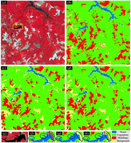
A 15-m multispectral ASTER image with 560 560 pixels is presented in Figure 3a. It contains four main land cover classes of water, vegetation, buildings, and bare ground. The training samples of the four classes were manually selected from Figure 3a for both pixel-based and object-based classifications. Training samples included 2338 pixels of water, 13,218 pixels of vegetation, 8005 pixels of buildings, and 1019 pixels of bare ground. These training samples were used as the inputs of pixel-based and object-based hard classifications to produce the PHC map in Figure 3b and the OHC map in Figure 3c. Meanwhile, the class proportions of pixels and objects were obtained by the soft support vector machine classifier with these training samples. IPOC took the class proportions of pixels and objects as its inputs to generate the IPOC map in Figure 3d. A stratified random sampling scheme was employed to select 2200 validation sites as test data from Figure 3a. Each validation site was first visually interpreted into a specific class, and then compared with PHC, OHC, and IPOC maps to compute confusion matrices and their indices of overall accuracy (OA), producer’s accuracy (PA), user’s accuracy (UA), and Kappa coefficient (KA) for quantitative accuracy assessment.
It can be found from Figure 3 that PHC preserved some small land cover patches and details but produced many isolated pixels. Some isolated pixels of buildings were evident in the PHC map of Figure 3b. By contrast, OHC avoided the salt and pepper effect caused by isolated pixels but lost some land cover details. It is clear that the isolated pixels of buildings in the PHC map were almost reduced in the OHC map of Figure 3c. Comparing the IPOC map with the PHC and OHC maps, IPOC generated less isolated pixels than PHC and preserved more land cover details than OHC. Using both pixel-based and object-based classifications, IPOC produced a more accurate classified map than PHC and OHC in visual examination, especially for the land cover details in intersection regions and small land cover patches. The results of the three methods in a subarea marked by a yellow rectangle in Figure 3a demonstrate this point. The IPOC result in Figure 3h displayed more accurate details than the OHC result of Figure 3g in the intersection regions between water and vegetation because OHC produced much over-classified water compared with the original ASTER image of Figure 3e. Meanwhile, IPOC preserved more accurate small bare ground and linear building patches than PHC and OHC at the right of the subarea in Figure 3h because PHC wrongly classified the small bare ground patch into buildings and OHC wrongly classified the small linear buildings into the class of bare ground.
Table 1 displays the quantitative accuracy assessment for the three classified maps of the ASTER image. The overall performance of IPOC was better than both PHC and OHC, and OHC was slightly better than PHC. Specifically, the OA of IPOC was 7.64% and 4.64% greater than PHC and OHC, respectively. At the same time, the KA of IPOC were 0.114 and 0.0731 higher than PHC and OHC, respectively. Focusing on individual classes, the PA of vegetation was significantly higher than the other three classes and the PA difference among the three maps was small. Although IPOC and PHC had nearly the same PA for water, they were clearly higher than OHC because of several omitted water patches in the OHC map. The PA increase of IPOC was evident in the two classes of buildings and bare ground. IPOC increased the PA of buildings by 5.54% and 5.06% over PHC and OHC, respectively. IPOC achieved the average PA increase of bare ground by 15.13%. The quantitative assessment further confirms the findings in the visual evaluation, especially for these improvements of buildings and bare ground classes.
3.2. Experiment on ZY-3 Imagery
A 5.8-m multispectral ZY-3 image (480 480 pixels) in Figure 4a was tested. This area also included four main land cover classes, namely water, vegetation, buildings, and bare ground. The training samples of the four classes were manually chosen from Figure 4a for classifications. Training samples included 1010 pixels of water, 3700 pixels of vegetation, 2888 pixels of buildings, and 2228 pixels of bare ground. These training samples were used in pixel-based and object-based hard classifications to generate the PHC map in Figure 4b and OHC map in Figure 4c. At the same time, the pixel-based and object-based soft classifications were performed to yield the class proportions of pixels and objects. They were used as inputs of IPOC to generate the IPOC map in Figure 4d. To quantitatively assess the PHC, OHC, and IPOC maps, 1700 validation sites were chosen as test data from Figure 4a by a stratified random sampling scheme. Each validation site was first manually interpreted into a specific class. Then, they were further compared with corresponding sites in PHC, OHC, and IPOC maps to compute confusion matrices and their indices.
As can be seen from Figure 4, the PHC map had a large number of salt and pepper pixels, especially in the two classes of buildings and bare ground while OHC effectively avoided the salt and pepper effect in Figure 4c. Despite this, PHC produced more accurate land cover details and small patches than OHC. For instance, Figure 4c had some wrongly classified small road patches in the same areas marked by two black ellipses in Figure 4d. The IPOC map in Figure 4d exhibits that it has less salt and pepper effect than the PHC map and more accurate land cover details than the OHC map. Especially, the small linear road patches in the two areas marked by two black ellipses in Figure 4d were preserved by IPOC. When visually comparing the original ZY-3 image in Figure 4a with the three classified maps, IPOC map is closer to the real spatial distribution of land cover than the other two maps in Figure 4b,c.
Table 2 shows the quantitative accuracy indices of PA, UA, OA, and KA for the three classified maps of the ZY-3 image. The accuracy assessment confirms the conclusion of visual evaluation. It can be seen that the overall performance of IPOC was better than both PHC and OHC, and the difference between PHC and OHC was very small. The average OA increase of IPOC was 3.5% and the KA of IPOC were 0.0528 and 0.0494 higher than PHC and OHC, respectively. As for single classes, the PA of each class achieved different improvements. Compared with PHC and OHC, the average PA increases of IPOC were 2.8%, 3.05%, 5.33%, and 2.64% for water, vegetation, buildings, and bare ground, respectively.
4. Discussion
4.1. Impact of Fusion Weight on IPOC Performance
Fusing the class proportion of pixels and the class spatial dependence of pixels was a critical process of IPOC. Thus, it was necessary to analyze the impact of the tradeoff between the class proportion and the class spatial dependence of pixels on the performance of IPOC. Here, ten different weights (from 0.05 to 0.95 with an interval of 0.1) of the class proportion of pixels were used to produce the IPOC maps for the ASTER image and ZY-3 image. The IPOC map of each weight was used to calculate its OA and these OAs were plotted in Figure 5 for each testing image. As can be observed from Figure 5, the OA curve reached the peak when the weight of the class proportions of pixels equaled 0.75 for the ASTER image. For the ZY-3 image, the maximum OA corresponded to the weight of 0.65. Therefore, the weights of 0.75 and 0.65 were applied to generate the final IPOC maps for the ASTER image and ZY-3 image, respectively. Figure 5 shows that the accuracy of IPOC gradually increased first and then decreased with the increase in the weight of the class proportions of pixels. It means that either object-based classification or pixel-based classification cannot effectively represent the land cover information and that the use of both pixel-based and object-based classifications is a more accurate way to represent land cover information. According to the two experimental results, the mapping of land cover details and small patches was mainly improved by IPOC. This is largely due to the fact that IPOC used pixel-scale and object-scale properties simultaneously. Meanwhile, IPOC provided more accurate classified results for mixed objects than both PHC and OHC. Besides, IPOC determined the class label of pixels in units of the object, which avoided some isolated pixels and preserved the land cover details simultaneously.
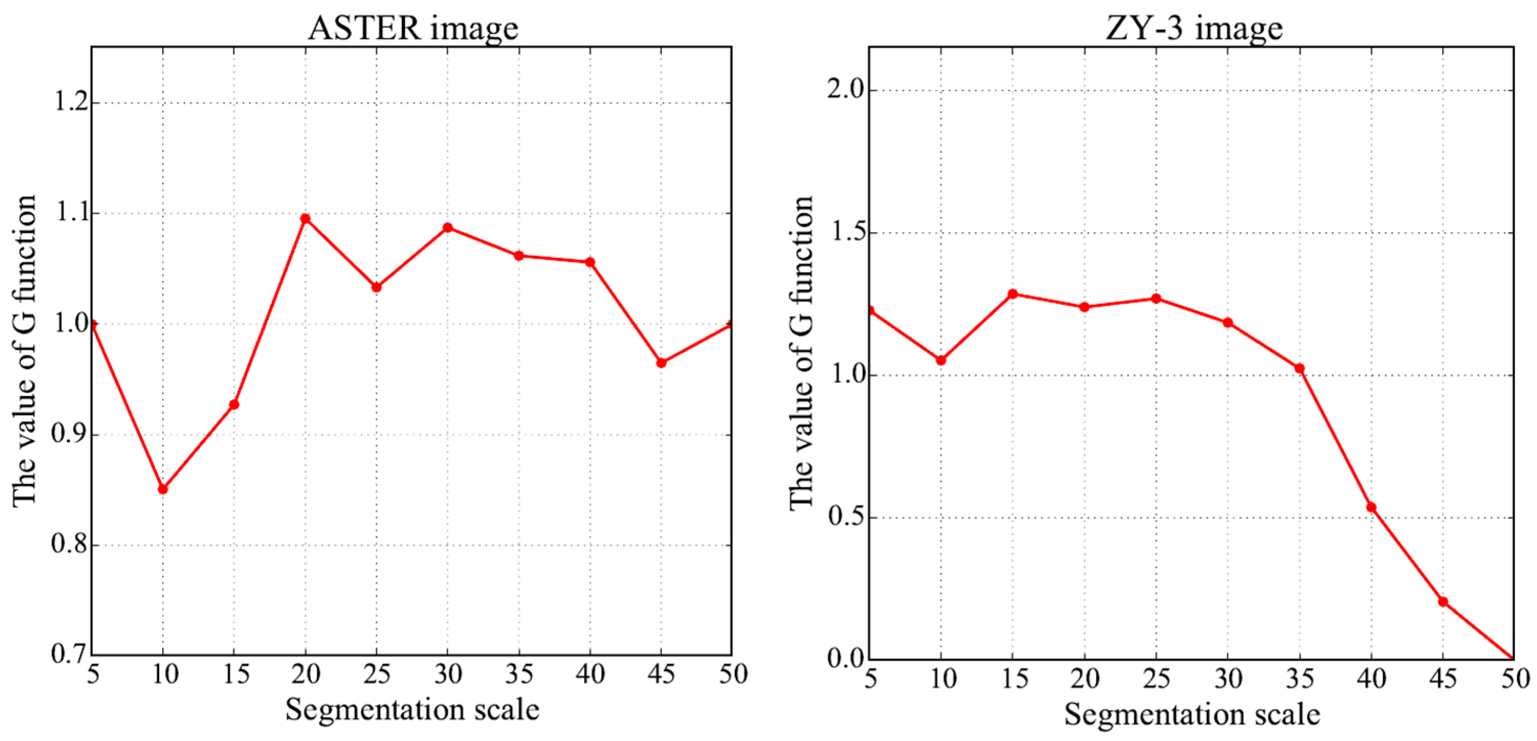
4.2. Analysis of Image Segmentation Scales
Image segmentation was considered as a crucial process in object-based classification [6]. It often required that several parameters be set, of which the segmentation scale was the most important [6]. The segmentation scale played a critical role in controlling the quality of the segmented objects and an optimal scale needed to be chosen in the process of image segmentation. Usually, the optimal segmentation scale generated the best image segmentation result [16]. Therefore, ten segmentation scales (from 5 to 50 with an interval of 5) were applied to the ASTER image and ZY-3 image. The optimal segmentation scale of each image was chosen from the ten scales by a segmentation quality assessment method. Segmentation quality assessment methods should consider the homogeneity within objects and the heterogeneity between objects [16]. Here, we used the function proposed in our previous work [13] to assess the quality of segmentation results and select the optimal segmentation scale for each image. The function combined the homogeneity within objects and heterogeneity between objects using Moran’s I values and objects’ variances and it achieved a satisfactory performance in selecting the optimal segmentation scales [13]. Figure 6 presents the function values in the y-axis with different segmentation scales in the x-axis. When the function reached the highest value, the corresponding segmentation scale was the optimal segmentation scale. As can be seen from Figure 6, the optimal segmentation scales were 20 and 15 for the ASTER image and ZY-3 image, respectively. Therefore, the selected optimal segmentation scales were used for both object-based classification and IPOC in the above two experiments. Note that the segmentation scale range from 5 to 50 was used in this study and different segmentation scale ranges may lead to different optimal segmentation scales. Compared with other studies [47,48], this scale range was relatively small. The selection of this scale range was based on the fact that the relatively small scale range may lead to a relatively small optimal scale for image segmentation. A relatively small scale may generate relatively less under-segmentation objects, which would result in mixed objects [49]. Therefore, the segmentation scale range from 5 to 50 was chosen to avoid lots of mixed objects. Although IPOC can effectively handle the mixed objects, the effectiveness of IPOC would be reduced if there were lots of large mixed objects generated by large scales in image segmentation. The reasons are that (1) IPOC inherits the basic idea of SRM and the performance of SRM is gradually decreased with an increase in scale factors [30,36,49], and (2) the class spatial dependence between objects are gradually reduced with an increase in object size [49]. The selection of the optimal segmentation scale depends on various factors (e.g., different remote sensing images and land surface complexity) [6]; therefore, the impact of different segmentation scales on IPOC can be discussed in the future.
4.3. Comparison between IPOC and the Other Method
IPOC was compared with traditional PHC and OHC in the two experiments and the experimental results show that IPOC outperformed both PHC and OHC. To further evaluate the effectiveness of IPOC, the majority rule-based method using pixel-based and object-based classifications was chosen to compare with IPOC [21,22]. The majority rule-based method first adopted PHC to produce the PHC result. Next, image objects were generated by image segmentation. Last, each object was allocated to a specific class that had the majority number of pixels within the object in PHC results. Here, the majority rule-based method was performed in the first experiment for the evaluation purpose. The result in Figure 3b was first used to calculate the pixel number of each class within an object, which was generated by the image segmentation of Figure 3a with the segmentation scale of 20. Then, the object was allocated to the class that had the maximum pixels within the object. The majority rule-based result was obtained when each object was labeled by a land cover class. The 2200 validation sites in the first experiment were also used to compute the confusion matrix of the majority rule-based result. The OA of the majority rule-based result was 83.68% and the KA was 0.7474, which was extracted from the confusion matrix. Compared with the majority rule-based method, the OA and KA of IPOC increased by 3.91% and 0.0584, respectively. The OAs of the majority rule-based method were 3.73% and 0.73% higher than PHC and OHC, respectively. When comparing with traditional PHC and OHC, the accuracy improvements of the majority rule-based method were slightly lower than those of IPOC. The main reason was that the majority rule-based result was affected by PHC and OHC results whereas IPOC not only took the advantages of PSC and OSC but also explored the class spatial dependence between objects to produce the detailed land cover information within mixed objects. Therefore, IPOC performed better than an existing classification method based on pixel-based and object-based classified results and the traditional PHC and OHC.
4.4. Uncertainty Analysis of Validation Data
Validation data played a critical role in quantitatively assessing classification results [50]. Validation sites were first chosen by a stratified random sampling scheme, and then each site was manually interpreted into a specific class for accuracy assessment. The selection and interpretation of validation sites had uncertainty for accuracy assessment. When the number of validation sites was set, each time the stratified random sampling scheme generated different validation sites, the accuracy assessment result may have had slight differences. Although there was uncertainty in generating validation sites, the accuracy assessment results would be stable in theory because of the stratified random sampling scheme [51]. The interpretation accuracy of validation sites varied depending on different experts. A recent study found that classifiers were more sensitive to geospatial label errors and a web-based labeling tool was introduced to avoid the geospatial label errors [50]. In this study, the interpretation process was completed by an expert. According to the web-based labeling tool, the expert zoomed in on each site to carefully consider the geospatial label of the site to avoid the labeling errors. Therefore, the label errors had slight impact on the accuracy assessment of PHC, OHC, and IPOC. Although the validation data had uncertainty, they affected only the quantitative accuracy assessment. In the two experiments, the visual evaluation of the classification results was carried out and indicates that the proposed IPOC method produced better classified image quality than both PHC and OHC.
5. Conclusions
This study aimed to propose a new classification method through integration of pixel-based and object-based classifications (IPOC) for dealing with the mixed object uncertainty problem. IPOC adopted pixel-based soft classification to produce the class proportions of pixels that were used to characterize the land cover details pixel by pixel. At the same time, IPOC explored the spatial relationships from object-based soft classification results and these spatial relationships between objects were employed to characterize the class spatial dependence of each pixel. The class proportions of pixels and the spatial dependence of pixels were combined further to produce a hard classification map by a linear optimization model in units of object. The results of the two experiments demonstrated that IPOC outperformed traditional pixel-based hard classification (PHC) and object-based hard classification (OHC). Therefore, IPOC is a new option for land cover mapping through the integration of pixel-based and object-based classifications.
In experiments, only two remote sensing images in small areas were used to assess the effectiveness of IPOC. In the future, IPOC can be conducted with more remote sensing images over larger areas in practical applications.
Acknowledgments
This work was supported in part by the National Natural Science Foundation of China under Grant 41701376 and Grant 41501453, in part by the Natural Science Foundation of Jiangsu Province under Grant BK20170866, in part by the Key Program of Chinese Academy of Sciences under Grant ZDRW-ZS-2016-6-3-4, in part by the Fundamental Research Funds for the Central Universities under Grant 2017B11714 and Grant 2016B11414, in part by the China Postdoctoral Science Foundation under Grant 2016M600356, and in part by the State Key Laboratory of Resources and Environmental Information System, China.
Author Contributions
Yuehong Chen and Ya’nan Zhou conceived and designed this study; Yuehong Chen performed the experiments and wrote the paper; Yong Ge, Ru An, and Yu Chen analyzed the experimental results and commented on the paper.
Conflicts of Interest
The authors declare no conflict of interest.
References
- Foody, G.M. Status of land cover classification accuracy assessment. Remote Sens. Environ. 2002, 80, 185–201. [Google Scholar] [CrossRef]
- Chen, J.; Chen, J.; Liao, A.; Cao, X.; Chen, L.; Chen, X.; He, C.; Han, G.; Peng, S.; Lu, M.; et al. Global land cover mapping at 30 m resolution: A pok-based operational approach. ISPRS J. Photogramm. Remote Sens. 2015, 103, 7–27. [Google Scholar] [CrossRef]
- Cihlar, J. Land cover mapping of large areas from satellites: Status and research priorities. Int. J. Remote Sens. 2000, 21, 1093–1114. [Google Scholar] [CrossRef]
- Tso, B.; Mather, P.M. Classification Methods for Remotely Sensed Data; CRC: Boca Raton, FL, USA, 2009. [Google Scholar]
- Fritz, S.; McCallum, I.; Schill, C.; Perger, C.; Grillmayer, R.; Achard, F.; Kraxner, F.; Obersteiner, M. Geo-wiki.Org: The use of crowdsourcing to improve global land cover. Remote Sens. 2009, 1, 345–354. [Google Scholar] [CrossRef]
- Blaschke, T.; Hay, G.J.; Kelly, M.; Lang, S.; Hofmann, P.; Addink, E.; Feitosa, R.Q.; van der Meer, F.; van der Werff, H.; van Coillie, F.; et al. Geographic object-based image analysis—Towards a new paradigm. ISPRS J. Photogramm. Remote Sens. 2014, 87, 180–191. [Google Scholar] [CrossRef] [PubMed]
- Lu, D.; Weng, Q. A survey of image classification methods and techniques for improving classification performance. Int. J. Remote Sens. 2007, 28, 823–870. [Google Scholar] [CrossRef]
- Shi, C.; Wang, L. Incorporating spatial information in spectral unmixing: A review. Remote Sens. Environ. 2014, 149, 70–87. [Google Scholar] [CrossRef]
- Duro, D.C.; Franklin, S.E.; Dube, M.G. A comparison of pixel-based and object-based image analysis with selected machine learning algorithms for the classification of agricultural landscapes using spot-5 hrg imagery. Remote Sens. Environ. 2012, 118, 259–272. [Google Scholar] [CrossRef]
- Lanorte, A.; De Santis, F.; Nole, G.; Blanco, I.; Loisi, R.V.; Schettini, E.; Vox, G. Agricultural plastic waste spatial estimation by landsat 8 satellite images. Comput. Electron. Agric. 2017, 141, 35–45. [Google Scholar] [CrossRef]
- Bialas, J.; Oommen, T.; Rebbapragada, U.; Levin, E. Object-based classification of earthquake damage from high-resolution optical imagery using machine learning. J. Appl. Remote Sens. 2016, 10, 036025. [Google Scholar] [CrossRef]
- Keyport, R.N.; Oommen, T.; Martha, T.R.; Sajinkumar, K.S.; Gierke, J.S. A comparative analysis of pixel- and object-based detection of landslides from very high-resolution images. Int. J. Appl. Earth Obs. Geoinf. 2018, 64, 1–11. [Google Scholar] [CrossRef]
- Chen, Y.; Ge, Y.; Jia, Y. Integrating object boundary in super-resolution land cover mapping. IEEE J. Sel. Top. Appl. Earth Obs. Remote Sens. 2016, 10, 219–230. [Google Scholar] [CrossRef]
- Wang, L.; Sousa, W.P.; Gong, P. Integration of object-based and pixel-based classification for mapping mangroves with ikonos imagery. Int. J. Remote Sens. 2004, 25, 5655–5668. [Google Scholar] [CrossRef]
- Liu, D.; Xia, F. Assessing object-based classification: Advantages and limitations. Remote Sens. Lett. 2010, 1, 187–194. [Google Scholar] [CrossRef]
- Espindola, G.M.; Camara, G.; Reis, I.A.; Bins, L.S.; Monteiro, A.M. Parameter selection for region-growing image segmentation algorithms using spatial autocorrelation. Int. J. Remote Sens. 2006, 27, 3035–3040. [Google Scholar] [CrossRef]
- Johnson, B.; Xie, Z.X. Unsupervised image segmentation evaluation and refinement using a multi-scale approach. ISPRS J. Photogramm. Remote Sens. 2011, 66, 473–483. [Google Scholar] [CrossRef]
- Fisher, P. The pixel: A snare and a delusion. Int. J. Remote Sens. 1997, 18, 679–685. [Google Scholar] [CrossRef]
- Woodcock, C.E.; Strahler, A.H. The factor of scale in remote sensing. Remote Sens. Environ. 1987, 21, 311–332. [Google Scholar] [CrossRef]
- Ge, Y.; Chen, Y.; Stein, A.; Li, S.; Hu, J. Enhanced sub-pixel mapping with spatial distribution patterns of geographical objects. IEEE Trans. Geosci. Remote Sens. 2016, 54, 2356–2370. [Google Scholar] [CrossRef]
- Li, X.J.; Meng, Q.Y.; Gu, X.F.; Jancso, T.; Yu, T.; Wang, K.; Mavromatis, S. A hybrid method combining pixel-based and object-oriented methods and its application in hungary using chinese hj-1 satellite images. Int. J. Remote Sens. 2013, 34, 4655–4668. [Google Scholar] [CrossRef]
- Costa, H.; Carrao, H.; Bacao, F.; Caetano, M. Combining per-pixel and object-based classifications for mapping land cover over large areas. Int. J. Remote Sens. 2014, 35, 738–753. [Google Scholar] [CrossRef]
- Malinverni, E.S.; Tassetti, A.N.; Mancini, A.; Zingaretti, P.; Frontoni, E.; Bernardini, A. Hybrid object-based approach for land use/land cover mapping using high spatial resolution imagery. Int. J. Geogr. Inf. Sci. 2011, 25, 1025–1043. [Google Scholar] [CrossRef]
- Aguirre-Gutierrez, J.; Seijmonsbergen, A.C.; Duivenvoorden, J.F. Optimizing land cover classification accuracy for change detection, a combined pixel-based and object-based approach in a mountainous area in mexico. Appl. Geogr. 2012, 34, 29–37. [Google Scholar] [CrossRef]
- Goncalves, L.M.S.; Fonte, C.C.; Julio, E.N.B.S.; Caetano, M. A method to incorporate uncertainty in the classification of remote sensing images. Int. J. Remote Sens. 2009, 30, 5489–5503. [Google Scholar] [CrossRef]
- Sheeren, D.; Bastin, N.; Ouin, A.; Ladet, S.; Balent, G.; Lacombe, J.P. Discriminating small wooded elements in rural landscape from aerial photography: A hybrid pixel/object-based analysis approach. Int. J. Remote Sens. 2009, 30, 4979–4990. [Google Scholar] [CrossRef] [Green Version]
- Aguilar, F.; Nemmaoui, A.; Aguilar, M.; Chourak, M.; Zarhloule, Y.; García Lorca, A. A quantitative assessment of forest cover change in the moulouya river watershed (morocco) by the integration of a subpixel-based and object-based analysis of landsat data. Forests 2016, 7, 23. [Google Scholar] [CrossRef]
- Atkinson, P.M. Mapping Sub-Pixel Boundaries from Remotely Sensed Images; Kemp, Z., Ed.; Taylor and Francis: London, UK, 1997; pp. 166–180. [Google Scholar]
- Boucher, A.; Kyriakidis, P.C. Super-resolution land cover mapping with indicator geostatistics. Remote Sens. Environ. 2006, 104, 264–282. [Google Scholar] [CrossRef]
- Foody, G.M.; Muslim, A.M.; Atkinson, P.M. Super-resolution mapping of the waterline from remotely sensed data. Int. J. Remote Sens. 2005, 26, 5381–5392. [Google Scholar] [CrossRef]
- Li, L.; Xu, T.; Chen, Y. Improved urban flooding mapping from remote sensing images using generalized regression neural network-based super-resolution algorithm. Remote Sens. 2016, 8, 625. [Google Scholar] [CrossRef]
- Li, X.; Ling, F.; Du, Y.; Zhang, Y. Spatially adaptive superresolution land cover mapping with multispectral and panchromatic images. IEEE Trans. Geosci. Remote Sens. 2014, 52, 2810–2823. [Google Scholar] [CrossRef]
- Ling, F.; Foody, G.; Li, X.; Zhang, Y.; Du, Y. Assessing a temporal change strategy for sub-pixel land cover change mapping from multi-scale remote sensing imagery. Remote Sens. 2016, 8, 642. [Google Scholar] [CrossRef]
- Mertens, K.C.; De Baets, B.; Verbeke, L.P.C.; de Wulf, R.R. A sub-pixel mapping algorithm based on sub-pixel/pixel spatial attraction models. Int. J. Remote Sens. 2006, 27, 3293–3310. [Google Scholar] [CrossRef]
- Tatem, A.J.; Lewis, H.G.; Atkinson, P.M.; Nixon, M.S. Multiple-class land-cover mapping at the sub-pixel scale using a hopfield neural network. Int. J. Appl. Earth Obs. Geoinf. 2001, 3, 184–190. [Google Scholar] [CrossRef]
- Wang, Q.; Atkinson, P.M. The effect of the point spread function on sub-pixel mapping. Remote Sens. Environ. 2017, 193, 127–137. [Google Scholar] [CrossRef]
- Xu, X.; Tong, X.; Plaza, A.; Zhong, Y.; Xie, H.; Zhang, L. Joint sparse sub-pixel mapping model with endmember variability for remotely sensed imagery. Remote Sens. 2017, 9, 15. [Google Scholar] [CrossRef]
- Zhang, Y.; Atkinson, P.M.; Li, X.; Ling, F.; Wang, Q.; Du, Y. Learning-based spatia-temporal superresolution mapping of forest cover with modis images. IEEE Trans. Geosci. Remote Sens. 2017, 55, 600–614. [Google Scholar] [CrossRef]
- Zhong, Y.; Wu, Y.; Xu, X.; Zhang, L. An adaptive subpixel mapping method based on map model and class determination strategy for hyperspectral remote sensing imagery. IEEE Trans. Geosci. Remote Sens. 2015, 53, 1411–1426. [Google Scholar] [CrossRef]
- Li, X.; Ling, F.; Foody, G.M.; Ge, Y.; Zhang, Y.; Du, Y. Generating a series of fine spatial and temporal resolution land cover maps by fusing coarse spatial resolution remotely sensed images and fine spatial resolution land cover maps. Remote Sens. Environ. 2017, 196, 293–311. [Google Scholar] [CrossRef]
- Goovaerts, P. Kriging and semivariogram deconvolution in the presence of irregular geographical units. Math. Geosci. 2008, 40, 101–128. [Google Scholar] [CrossRef]
- Truong, N.P.; Heuvelink, G.B.M.; Pebesma, E. Bayesian area-to-point kriging using expert knowledge as informative priors. Int. J. Appl. Earth Obs. Geoinf. 2014, 30, 128–138. [Google Scholar] [CrossRef]
- Chen, Y.; Ge, Y.; Wang, Q.; Jiang, Y. A subpixel mapping algorithm combining pixel-level and subpixel-level spatial dependences with binary integer programming. Remote Sens. Lett. 2014, 5, 902–911. [Google Scholar] [CrossRef]
- Chen, Y.; Ge, Y.; Heuvelink, G.B.M.; Hu, J.; Jiang, Y. Hybrid constraints of pure and mixed pixels for soft-then-hard super-resolution mapping with multiple shifted images. IEEE J. Sel. Top. Appl. Earth Obs. Remote Sens. 2015, 8, 2040–2052. [Google Scholar] [CrossRef]
- Chen, Y.; Ge, Y.; Song, D. Superresolution land-cover mapping based on high-accuracy surface modeling. IEEE Geosci. Remote Sens. Lett. 2015, 12, 2516–2520. [Google Scholar] [CrossRef]
- Guo, X.; Huang, X.; Zhang, L.; Zhang, L.; Plaza, A.; Benediktsson, J.A. Support tensor machines for classification of hyperspectral remote sensing imagery. IEEE Trans. Geosci. Remote Sens. 2016, 54, 3248–3264. [Google Scholar] [CrossRef]
- Martha, T.R.; Kerle, N.; Jetten, V.; van Westen, C.J.; Kumar, K.V. Characterising spectral, spatial and morphometric properties of landslides for semi-automatic detection using object-oriented methods. Geomorphology 2010, 116, 24–36. [Google Scholar] [CrossRef]
- Martha, T.R. Detection of Landslides by Object-Oriented Image Analysis; The University of Twente: Enschede, The Netherlands, 2011. [Google Scholar]
- Chen, Y.; Ge, Y.; Heuvelink, G.B.M.; An, R.; Chen, Y. Object-based superresolution land cover mapping from remotely sensed imagery. IEEE Trans. Geosci. Remote Sens. 2018, 56, 328–340. [Google Scholar] [CrossRef]
- Frank, J.; Rebbapragada, U.; Bialas, J.; Oommen, T.; Havens, T.C. Effect of label noise on the machine-learned classification of earthquake damage. Remote Sens. 2017, 9, 803. [Google Scholar] [CrossRef]
- Esfahani, M.S.; Dougherty, E.R. Effect of separate sampling on classification accuracy. Bioinformatics 2014, 30, 242–250. [Google Scholar] [CrossRef] [PubMed]
Figure 1.
Mixed objects. (a) A high-resolution type mixed object where the size of the segmented object with the red boundary is smaller than that of the water object; (b) A low-resolution type mixed object where the size of the segmented object with the red boundary is larger than that of its inner isolated patch.

Figure 2.
Flowchart of the integration of pixel-based and object-based classifications (IPOC).

Figure 3.
Experimental results of the 15-m ASTER image. (a) Multispectral ASTER image; (b) pixel-based hard classification (PHC) result; (c) object-based hard classification (OHC) result; and (d) IPOC result. (e–h) Maps from (a–d) in the yellow rectangle subarea, respectively.
Figure 3.
Experimental results of the 15-m ASTER image. (a) Multispectral ASTER image; (b) pixel-based hard classification (PHC) result; (c) object-based hard classification (OHC) result; and (d) IPOC result. (e–h) Maps from (a–d) in the yellow rectangle subarea, respectively.
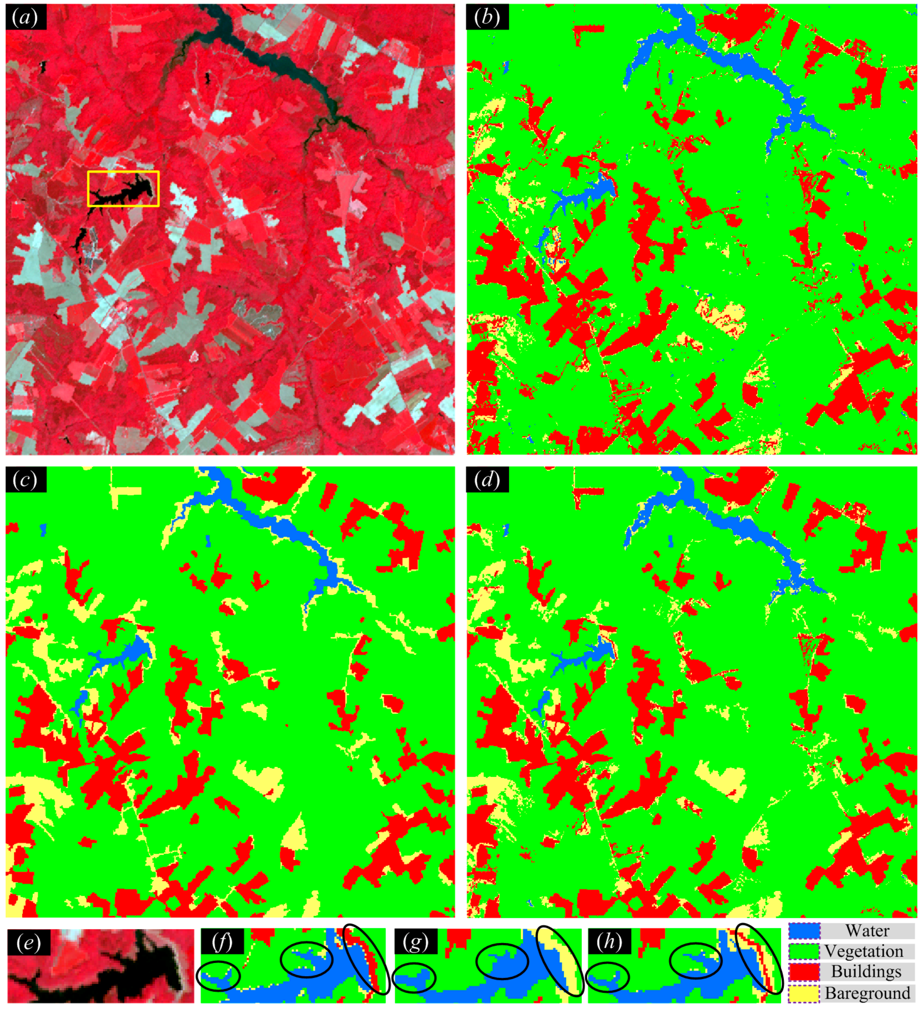
Figure 4.
Experimental results of the 5.8-m ZY-3 image. (a) Multispectral ZY-3 image; (b) PHC result; (c) OHC result; and (d) IPOC result.
Figure 4.
Experimental results of the 5.8-m ZY-3 image. (a) Multispectral ZY-3 image; (b) PHC result; (c) OHC result; and (d) IPOC result.
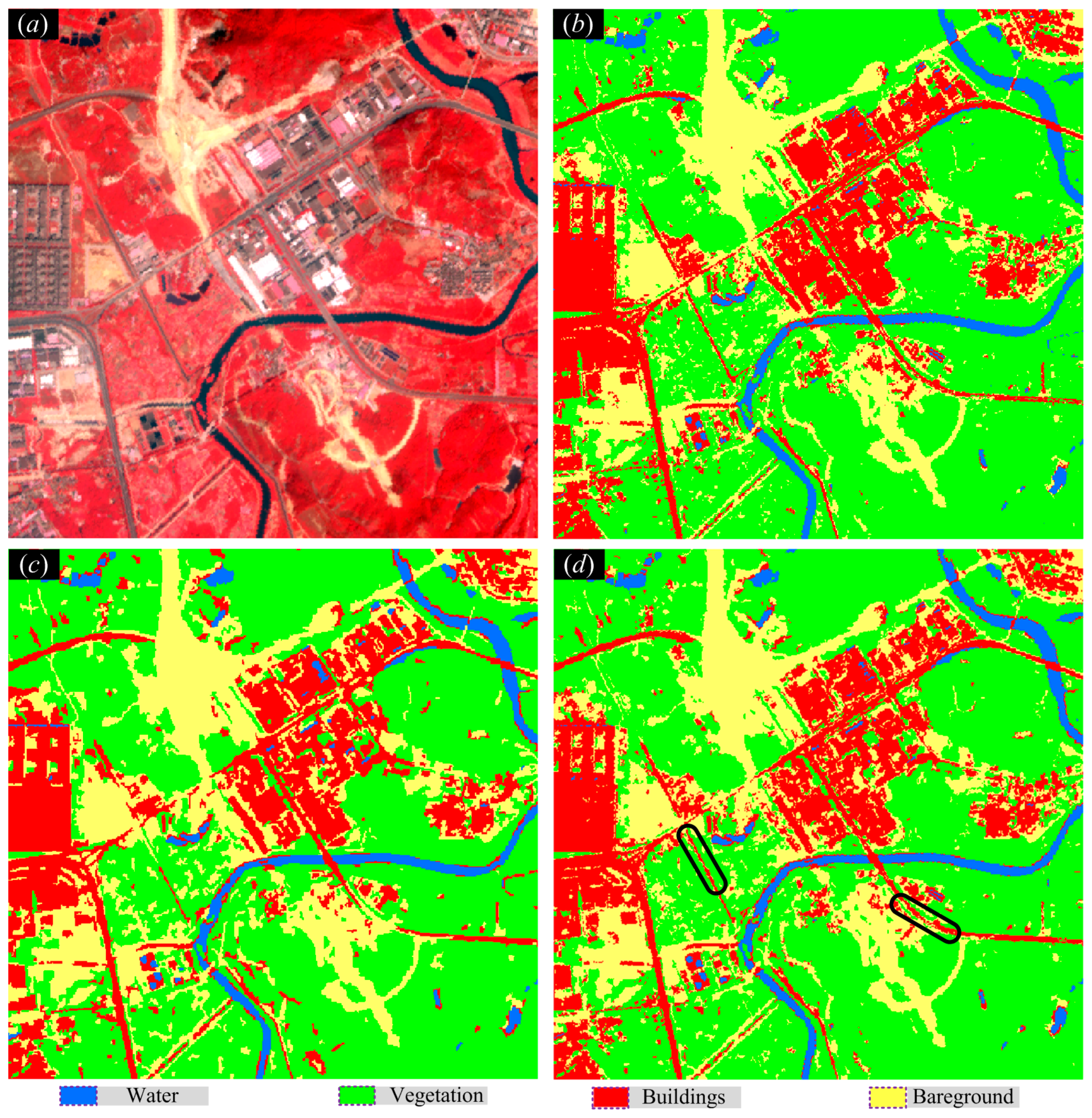
Figure 5.
The impact of different weights of the class proportions of pixels on IPOC.

Figure 6.
The optimal segmentation scales for the ASTER image and ZY-3 image.

Table 1.
Accuracy assessment for the ASTER image.
| Method | Water | Vegetation | Buildings | Bare Ground | |
|---|---|---|---|---|---|
| PHC | PA (%) | 77.25 | 92.07 | 79.04 | 55.11 |
| UA (%) | 75.26 | 86.77 | 66.67 | 78.57 | |
| OA (%) = 79.95 | KA = 0.6918 | ||||
| OHC | PA (%) | 68.78 | 94.17 | 79.52 | 66.53 |
| UA (%) | 80.25 | 83.85 | 90.66 | 75.11 | |
| OA (%) = 82.95 | KA = 0.7327 | ||||
| IPOC | PA (%) | 77.78 | 95.72 | 84.58 | 75.95 |
| UA (%) | 97.35 | 86.14 | 90.93 | 85.36 | |
| OA (%) = 87.59 | KA = 0.8058 | ||||
PA: producer’s accuracy, UA: user’s accuracy, OA: overall accuracy, and KA: Kappa coefficient.
Table 2.
Accuracy assessment for the ZY-3 image.
| Method | Water | Vegetation | Buildings | Bare Ground | |
|---|---|---|---|---|---|
| PHC | PA (%) | 80.68 | 83.78 | 75.54 | 79.42 |
| UA (%) | 92.21 | 88.30 | 78.00 | 67.64 | |
| OA (%) = 80.65 | KA = 0.7074 | ||||
| OHC | PA (%) | 81.82 | 84.27 | 73.61 | 81.00 |
| UA (%) | 88.89 | 89.51 | 83.52 | 63.56 | |
| OA (%) = 80.82 | KA = 0.7108 | ||||
| IPOC | PA (%) | 84.09 | 87.07 | 79.90 | 82.85 |
| UA (%) | 100.00 | 88.81 | 87.77 | 70.40 | |
| OA (%) = 84.24 | KA = 0.7602 | ||||
PA: producer’s accuracy, UA: user’s accuracy, OA: overall accuracy, and KA: Kappa coefficient.
© 2018 by the authors. Licensee MDPI, Basel, Switzerland. This article is an open access article distributed under the terms and conditions of the Creative Commons Attribution (CC BY) license (http://creativecommons.org/licenses/by/4.0/).
Share and Cite
MDPI and ACS Style
Chen, Y.; Zhou, Y.; Ge, Y.; An, R.; Chen, Y. Enhancing Land Cover Mapping through Integration of Pixel-Based and Object-Based Classifications from Remotely Sensed Imagery. Remote Sens. 2018, 10, 77. https://doi.org/10.3390/rs10010077
AMA Style
Chen Y, Zhou Y, Ge Y, An R, Chen Y. Enhancing Land Cover Mapping through Integration of Pixel-Based and Object-Based Classifications from Remotely Sensed Imagery. Remote Sensing. 2018; 10(1):77. https://doi.org/10.3390/rs10010077
Chicago/Turabian StyleChen, Yuehong, Ya’nan Zhou, Yong Ge, Ru An, and Yu Chen. 2018. "Enhancing Land Cover Mapping through Integration of Pixel-Based and Object-Based Classifications from Remotely Sensed Imagery" Remote Sensing 10, no. 1: 77. https://doi.org/10.3390/rs10010077
Note that from the first issue of 2016, this journal uses article numbers instead of page numbers. See further details here.