Wind in Complex Terrain—Lidar Measurements for Evaluation of CFD Simulations

1
Department of Energy and Process Engineering, Norwegian University of Science and Technology, 7491 Trondheim, Norway
2
Meventus AS, 4630 Kristiansand, Norway
3
Fraunhofer-Institute for Wind Energy and Energy System Technology, IWES, 26129 Oldenburg, Germany
*
Author to whom correspondence should be addressed.
Remote Sens. 2018, 10(1), 59; https://doi.org/10.3390/rs10010059
Submission received: 13 November 2017
/
Revised: 21 December 2017
/
Accepted: 28 December 2017
/
Published: 4 January 2018
(This article belongs to the Special Issue Remote Sensing of Atmospheric Conditions for Wind Energy Applications)
Abstract
:Computational Fluid Dynamics (CFD) is widely used to predict wind conditions for wind energy production purposes. However, as wind power development expands into areas of even more complex terrain and challenging flow conditions, more research is needed to investigate the ability of such models to describe turbulent flow features. In this study, the performance of a hybrid Reynolds-Averaged Navier-Stokes (RANS)/Large Eddy Simulation (LES) model in highly complex terrain has been investigated. The model was compared with measurements from a long range pulsed Lidar, which first were validated with sonic anemometer data. The accuracy of the Lidar was considered to be sufficient for validation of flow model turbulence estimates. By reducing the range gate length of the Lidar a slight additional improvement in accuracy was obtained, but the availability of measurements was reduced due to the increased noise floor in the returned signal. The DES model was able to capture the variations of velocity and turbulence along the line-of-sight of the Lidar beam but overestimated the turbulence level in regions of complex flow.
1. Introduction
In recent years, computational fluid dynamics (CFD) have frequently been applied for predicting wind conditions in the wind energy industry. Such flow models can provide a three-dimensional description of the flow field in a large area using input data from point measurements or meso-scale meteorological models. However, although CFD models have become increasingly advanced, the challenge of accurately describing turbulent flow, e.g., in complex terrain, remains. For a large three-dimensional area, the requirement of spatial and temporal resolution to accurately resolve turbulent structures is simply not computationally affordable. An approach that has proved to yield valuable results for turbulence prediction is the Large Eddy Simulation (LES) method, which separates the flow in large and small scale eddies to save computational effort [1].
Research has been done regarding the performance of various LES models for describing turbulent wind conditions in complex terrain. A comprehensive blind test including several models, called the Bolund experiment, has been conducted by Bechmann et al. [1], where the accuracy of these models across an isolated hill was tested. The performance of the LES models included in the analysis yielded somewhat disappointing results with significant speed-up errors over the Bolund Hill. One reason for the large deviations might be the challenge of obtaining the correct free stream boundary condition, which the LES models failed to do in this study [1]. A similar experiment has been done by Bechmann and Sørensen [2], where a hybrid Reynolds-Averaged Navier-Stokes (RANS)/Large Eddy Simulation (LES) model was tested over the Askervein Hill in Scotland. In this model, the near-wall regions are resolved in a Reynolds-Averaging manner with the two-equation k-Epsilon turbulence model. The model was able to predict the high turbulence level in the complex wake region downwind of the hill reasonably well, but underestimated the mean velocity [2].
Experiments like Askervein Hill and Bolund Hill have provided invaluable insights into flow model performance and provided a benchmark for further flow model development. However, as wind power development expands into areas of even more complex terrain and challenging flow conditions, there is a need for full-scale validation cases, which reflects the challenges the wind industry meets today. This paper presents a validation case in highly complex terrain, using a pulsed Doppler Lidar. Lidars are particularly useful for this purpose as they can measure the spatial distribution of the wind along the Lidar beam. However, there are limitations in the Lidar technology that need to be addressed in order to make the measurements useful for flow model validation purposes.
One of the main limitations of the Lidar technology is that a horizontally homogeneous velocity field is assumed when deriving the three-dimensional wind field, which is not a valid assumption in complex terrain. Several studies regarding the performance of Lidars in complex terrain have been conducted, among others by Guillén et al. [3] and Vogstad et al. [4]. Guillén et al. found that the deviation between ten-minute averaged Lidar and cup anemometer measurements was significantly larger when the wind direction was such that the complex terrain features were most prominent. A greater discrepancy was also observed for higher turbulence intensities, and for higher vertical velocities [3]. Vogstad et al. [4] tested the performance of three different Lidars—WindCube V1, ZephIR 300 and Galion/StreamLine in complex terrain by comparing measurements with cup anemometer data. A numerical flow model was used to correct for the inhomogeneities of the terrain when deriving the three-dimensional velocity field. They found that the uncertainty of the ten-minute averaged velocities from all Lidars were in the order of 2.5% when applying the appropriate numerical corrections, which is comparable to the uncertainty of cup anemometers [4]. However, none of the Lidar instruments were found to predict the ten-minute averaged horizontal turbulence intensity accurately.
Lidar systems are also limited by spatial averaging along the Lidar beam. This effect is most prominent in the accuracy of turbulence estimations when small fluctuations are of vital importance. Several studies have investigated the ability of Lidar systems to provide accurate one-dimensional turbulence statistics, and methods such as the one described by Lenschow et al. [5] can be applied to improve the accuracy of these estimates under the assumption of isotropic turbulence. Bonin et al. [6] shows how measurement noise in Lidar data can be treated to improve the turbulence estimates. They investigated the performance of a StreamLine and WindCube Lidar compared to a sonic anemometer, and applied the methods of Lenschow to correct for white noise and limitations of spatiotemporal averaging of the measurements. Sjöholm et al. [7] investigated the spatial averaging effect for a ZephIR continuous-wave Lidar by comparing one-dimensional velocities with sonic measurements projected onto the line-of-sight (LOS) of the Lidar. Two periods with different atmospheric conditions were investigated—one with low clouds and high backscattering, and one with clear conditions. The power density spectra were almost identical for low frequencies, but the Lidar spectrum fell off more rapidly than the sonic spectrum for higher frequencies in both cases, proving that the Lidar did not capture the small-scale turbulent features of the wind as accurately as the sonic anemometer. The spectra deviated at approximately 0.02 Hz in the clear conditions case and 0.05 Hz in the low cloud case with stronger backscattering. Cañadillas et al. [8] investigated the same effect for a WindCube pulsed Lidar with a range gate length of 20 m on an offshore site. In this case, the power density spectra for line-of-sight velocities from the Lidar and the sonic anemometer were only comparable up to a frequency of 0.21 Hz due to the scanning pattern of the Lidar. The spectra showed a good compliance, and it was concluded that the spatial averaging along the Lidar beam had a negligible effect for this range of frequencies.
Although Lidars have become widely used in wind energy applications [9], they can only provide a relatively accurate estimate of turbulence along the line of sight. Multi-Lidar systems are capable of addressing this shortcoming [10,11]; however, these systems can still only measure the three-dimensional wind in one point at a time.
The lack of ability to provide a three-dimensional estimate of atmospheric turbulence limits the applicability of Lidar systems for evaluation of wind turbine structural integrity in complex terrain, where flow homogeneity and isotropic turbulence cannot be assumed. Therefore, CFD flow models are widely used to evaluate the spatial distribution of turbulence in complex terrain. However, such models are often only validated against point measurements, being meteorological masts or Lidars operating in Velocity azimuth display (VAD) mode. Using the method proposed in this paper, we believe that a pulsed Lidar, capable of measuring higher-order statistics of the wind along the line of sight, can be used efficiently to improve the accuracy of the flow models used in the industry today.
In this study, we have used a free-scanning Lidar operating in fixed direction stare-mode aligned with the mean flow direction. This way, accurate estimations of the wind fluctuations along the line-of-sight may be derived, which can be used to validate how the flow model predicts the variations of turbulence in the mean flow along the same line. The results can also give an indication of where the model succeeds or fails in predicting turbulence transport, production or dissipation.
The main objectives of this study are to (1) evaluate the accuracy of 1D Lidar measurements with a focus on turbulence estimation; (2) investigate how reduced gate length may increase the accuracy of turbulence estimations with the Lidar; and (3) use the Lidar data to validate a computational flow model in highly complex terrain. Lidar line-of-sight measurements will be validated with sonic anemometer data projected onto the Lidar beam, and the effect of spatial averaging will be investigated by changing the range gate length of the Lidar. For the flow model validation, a hybrid RANS/LES (DES) model will be applied along a horizontal Lidar beam parallel to the mean flow.
2. Materials and Methods
The measurement campaign was carried out by Meventus in Roan in Sør-Trøndelag, Norway, with a ground-based StreamLine XR pulsed Lidar in the proximity of a meteorological mast. The Lidar system is capable of recording raw data, making it possible to reprocess the data to provide time series with different gate lengths and frequencies. The system is operated with a collimated output beam, and the full width at half maximum (FWHM) is about 35 m. The instrument is described in more detail in Pearson et al. [12]. In the following sections, a brief description of the site will be provided before the setup of the instruments and the methodology of the analysis will be explained.
2.1. Site Description
The site is located in central Norway, approximately 3 km from the coastline. The terrain at the site is complex, with rocky, mountainous and open topography. A steep ridge located 1300 m west of the Lidar and mast is expected to generate complex flow with large-scale turbulent eddies. The positions of the Lidar and mast, and the surrounding terrain are shown in Figure 1.
2.2. Experimental Setup for Lidar Validation
The triangular lattice mast is located at 366 meters above sea level (m a.s.l.). The instrumentation installed on the mast are summarized in Table 1. The StreamLine XR v14-8 Lidar is located 344 m north of the mast at 370 m a.s.l. The range gate length of the Lidar was set to 18 m.
In order to avoid movement of the Lidar in strong winds, the Lidar was bolted to the ground using rock anchors. The instrument was leveled and oriented towards north using binoculars with compass. Lidar roll and tilt was logged throughout the campaign. The Lidar bearing was determined by scanning towards the mast and identifying at what azimuth backscatter from the mast was observed. The Lidar bearing was confirmed at the end of the measurement program, in order to confirm that no drift occurred.
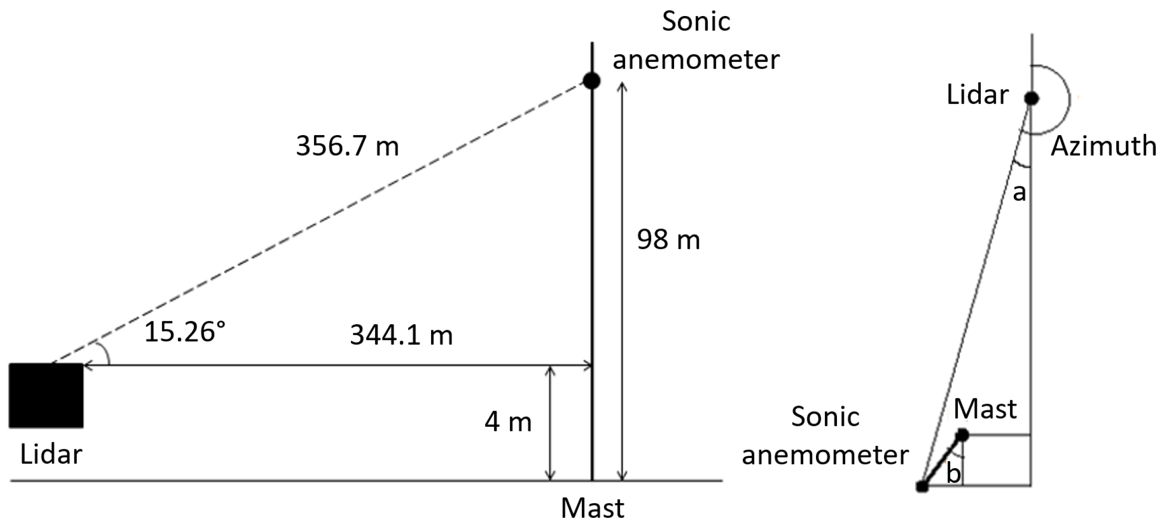
Line-of-sight velocities from the Lidar were collected with a sampling frequency of 1 Hz throughout a two-month period from 13 April 2015 to 11 June 2015. Corresponding horizontal and vertical velocities and wind directions were collected with the sonic anemometer at 98 m height for the same period. Due to inaccuracies in alignment tools for the sonic anemometer, an offset in the alignment of −7° was detected and corrected for. The offset was determined through a correlation analysis determining the offset required to obtain the highest correlation between the Lidar and the corresponding decomposed sonic signal. Figure 2 illustrates the setup of the two instruments.
Data Analysis
The sonic anemometer measurements were projected onto the line-of-sight of the Lidar to allow for a comparison of one-dimensional velocities along the Lidar beam. As the elevation angle is fairly large, a 3D projection was applied to account for the vertical velocity component.
To provide information about the quality of the Lidar data, these include values for the pitch and roll angles and the signal-to-noise ratio (SNR) of the backscattered signal. The pitch and roll angles are the forward/backward and sideways tilt angles of the Lidar. During the measurement period, these were checked remotely to be within a 0.25° threshold. This yields a maximum deviation of 1.55 m of the beam from the sonic anemometer. When validating the Lidar data, a stronger filtration of these values was performed to ensure that the beam deviation was within 1 m, corresponding to a maximum 0.16° pitch and roll angle. An analysis was carried out to determine how the correlation of the Lidar and sonic anemometer data was affected by filtration of SNR values. Although recent studies [6,13] have shown that the spatial averaging effects of the Lidar can be corrected to some extent, none of these methods were applied. The aim of this study was to verify that the Lidar is sufficiently accurate to validate numerical models in complex terrain. As the uncertainty involved in numerical models is generally much higher than the Lidar uncertainty, additional corrections were considered to be outside the scope of this study.
Velocity measurements and turbulence estimates were compared using standard linear regression analysis. The coefficient of determination R2, defined by Equation (1) [14] for data sets x and y, was used as a measure of the correlation between the Lidar and sonic anemometer measurements, respectively:
A spectral analysis was performed for a more detailed comparison of the data. Power density spectra illustrate how the energy is transferred from larger to smaller eddies. As a reference, the spectra were compared with the theoretical Kolmogorov slope of in the inertial subrange [15].
The effect of changing the range gate length of the Lidar was investigated by reprocessing raw Lidar data in the program Raw Data Processor v14 developed by Halo Photonics (Worcestershire, UK). A 24 h period on 30 April 2015 with large variations in wind velocity and direction was chosen for this analysis to challenge the Lidar with varying wind conditions. The wind velocity and direction measured by the sonic anemometer during this period are illustrated in Figure 3. Data were reprocessed with range gate lengths of 9 m and 30 m.
Throughout the entire analysis, only coinciding data from the Lidar and the sonic anemometer were used. For periods when Lidar data were not available due to filtration requirements, the sonic anemometer data were also removed. This data removal causes the spectra to appear with certain artifacts, as the resulting time series does not represent the physical processes in the atmosphere. However, the spectra will be suitable for evaluating the ability of the Lidar system to represent high-frequency wind speed variations.
2.3. Experimental Setup for the Flow Model Validation
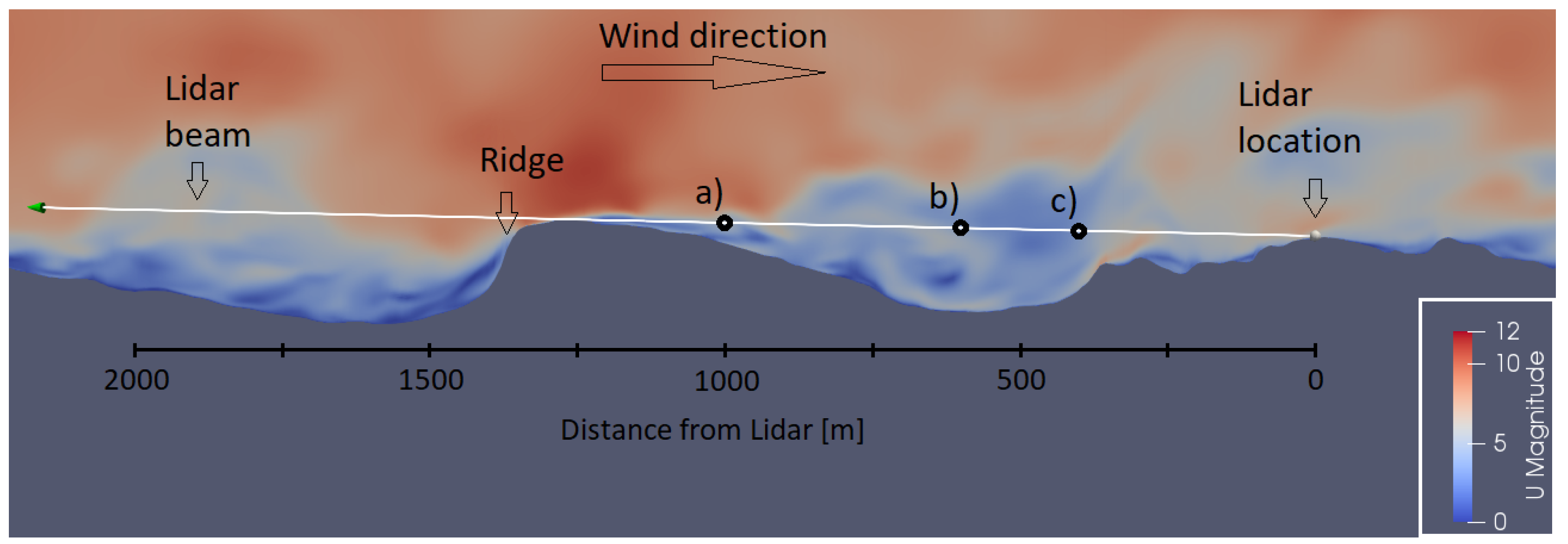
The large-scale turbulent structures of interest in this study are expected to be generated downwind of the ridge located approximately 1300 m southwest of the Lidar. The ridge has a steep vertical cliff with an elevation of 150 m facing westward. For the purpose of validating the flow models, the Lidar was operating in stare-mode towards this ridge, with an azimuth of 262°, parallel to the mean flow. This corresponds to an azimuth of 259.70° relative to grid north (UTM zone 32, WGS 84). (The use of grid north as the reference is chosen in order to avoid differences between the coordinate system of the flow model and the Lidar.) The velocity was measured along the length of the beam, and the locations (a)–(c) shown in Figure 4 were used for a more detailed spectral analysis.
A detailed assessment of wind data from the mast was used to identify a period with steady wind speeds and wind direction approximately orthogonal to the ridge. The estimated Monin–Obukhov length scale [16] was found to be near-neutral () for the entire period, implying that the vertical heat flux is close to zero. The conditions during the selected time period are presented in Table 2.
Lidar alignment was verified by pointing the Lidar beam towards the hill at different elevations, obtaining solid target return values where the Lidar beam hit the terrain. The Lidar beam was aligned to pass approximately 5 m over the crest of the hill, with an elevation angle of 2°. Analysis of the variations in pitch and roll during the experiment showed that the variation in elevation of the Lidar beam was on the order of 0.2 degrees. This corresponds to ±4.4 m at the crest of the hill.
Results from the flow models were extracted along a line that started at the position of the Lidar and passed through a point 5 m above the digital terrain elevation at the crest of the hill. The azimuth was kept at 259.7° for the evaluations of the mean flow field.
Simulation Procedure
Classical methodology regarding wind farm modeling using computational fluid dynamics (CFD) refers to two general strategies: the Reynolds–Averaged Navier–Stokes (RANS) and Large Eddy Simulation (LES) methods. In the RANS method, the simulation is executed aiming for a steady state solution, for which the turbulent properties are modeled in the framework of applied transport models. As a result, the transient behavior of turbulent flows is suppressed. The general principle of the LES method is to resolve the turbulent structures in the mean flow, i.e., the large eddies, and model the effect of the smaller eddies. Although this approach will yield more realistic results, the computational cost is much higher [17].
Due to the filtering of large and small eddies, LES models encounter severe difficulties in the near-wall region, for which the correct physical characteristics cannot be reproduced due to insufficient mesh resolution. This is a significant problem for atmospheric boundary layer flows with high Reynolds numbers, as the mesh requirement becomes computationally unaffordable. To solve this issue, a Detached Eddy Simulation (DES) is used in this study. A DES is a hybrid RANS/LES method, which compensates this shortcoming by applying the RANS model in the near-wall region. The switch from LES to RANS is based on the to-wall distance, as well as the modeling length scale and cell size [2]. The hybrid RANS/LES approach selected for this numerical study was first proposed by Spalart [17]. Details about the transport models, as well as the filtering strategies are described by Bechmann et al. [2]. The traditional RANS model is also included in the analysis for comparison.
The computational domain was constructed by Fraunhofer Institute for Wind Energy and Energy System Technology’s (IWES) terrainMesher (Oldenburg, Germany), and the simulations were performed by Fraunhofer IWES in OpenFOAM (version 2.3.1, OpenCFD Ltd, Bracknell, UK). A region covering a 9.5 km × 7.3 km area orthogonal to the wind direction was meshed by ∼56 million degrees of freedom, with increasing mesh resolution near the surface. The governing equation system is the Navier–Stokes equations, and the RANS and DES flow models are applied without heat transfer (neutral conditions).
The inlet condition with a mean bulk velocity of 8.3 m/s was first estimated by a RANS simulation using the k-Epsilon turbulence model. This model is widely used in the wind energy industry today, and serves as a baseline for the evaluation of the DES model. The RANS model also served as the starting point for the DES simulation. However, to obtain the required eddy structures in the inlet profile for the DES simulation, a prolonged inlet with circulating flow was used. The velocity fluctuations were triggered by surface shear, which caused an instability in the momentum equation. The domain with the prolonged inlet is shown in Figure 5.
The DES simulation was executed over 25,000 physical seconds, which corresponds to approximately 20 flow through times (FTT). The results were averaged over 15 FTT, which can demonstrate a plausible statistical representation.
A spectral analysis was performed for a few locations along the beam. The spectra were compared with the predicted Kaimal spectrum for the longitudinal wind speed, which is given by Equation (2) [18]:
is the friction velocity, is the power density for the longitudinal wind and f is the normalized frequency, related to frequency n, height z and velocity U(z) by relation (3):
3. Results
In this section, a validation of the Lidar will be presented by comparison with sonic anemometer data. Next, the effect of changing the range gate length of the Lidar will be analyzed. At last, the Lidar measurements will be used to validate the performance of a RANS and DES flow model.
3.1. Validation of Lidar Measurements
For evaluating the accuracy of turbulence estimates with the Lidar, the data were compared to sonic anemometer measurements with a sampling frequency of 1 Hz. As an initial analysis, the effect of the level of filtration of Lidar data was investigated. Noisy measurements were removed by increasing the filtering limit on the Signal-to-noise ratio (SNR) value of the Lidar signals, and the correlation between the Lidar and sonic anemometer data were evaluated by incrementally increasing the SNR filter value by 0.01 for each step. Figure 6 shows how the coefficient of determination changes with the limiting SNR value, and how the availability of measurements is affected.
The figure shows that the coefficient of determination has a maximum value of R2 = 0.9454 with an optimal SNR limit of −10 dB. The slope of the linear regression line for this limit is 0.9705. With a higher limit, the reduction of availability will dominate and cause a decrease in the coefficient of determination. This effect occurs because the differences between the Lidar and sonic anemometer measurements are amplified for large and rapid changes in velocity, which typically occurs across long time gaps.
When increasing the SNR limit, periods with clear conditions are also filtered out. Figure 7 illustrates how the relative humidity and SNR are related. In clear conditions with low humidity, the SNR is low due to a weak backscattering. When the humidity increases, the aerosols swell and the backscattering is increased [21]. With the optimal SNR limit of −10 dB, the availability is reduced to 74.2% due to a loss of such periods. The figure only shows a time period of 24 h on 30 April 2015, but the illustrated phenomenon is applicable for all times and causes a loss of clear-condition periods with higher SNR limits.
In Figure 8, the one-dimensional wind velocity measured with the Lidar and the sonic anemometer with a sampling frequency of 1 Hz and the optimal SNR limit of −10 dB are plotted as a function of time. Due to clear conditions during the first four days, these data have been filtered out with an SNR limit of −10 dB. The Lidar measurements follow the sonic measurements very well, although the sonic anemometer captures more fluctuations than the Lidar. As explained in Section 1, the spatial averaging along the Lidar beam removes some of the small-scale features of the wind, and hence the small fluctuations are not described as accurately as with the sonic anemometer. Similar results were observed by Sjöholm et al. [7].
Figure 9 shows a correlation plot of one-dimensional ten-minute averaged velocities from the Lidar and the sonic anemometer. The coefficient of determination during this period is R2 = 0.9972, and the linear regression slope is 1.0043. The figure confirms the Lidars’ ability to obtain accurate mean velocities. The ten-minute averaged velocities correlate almost perfectly and are comparable with results from similar experiments done in previous research [4,22].
Figure 10 shows a correlation plot with the optimal SNR limit of −10 dB and a sampling frequency of 1 Hz. There is a larger spread in this case than for the ten-minute averaged velocities in Figure 9, which is also reflected in the lower coefficient of determination R2 = 0.9454 and slope of the linear regression line 0.9705. The spread does not necessarily represent a flaw in the instruments, but rather a physically different approach to wind speed estimation. While the sonic anemometer is close to a point measurement, the Lidar measures the wind over a larger volume.
In Figure 11, the ten-minute mean standard deviations along the line-of-sight estimated by the Lidar and the sonic anemometer are plotted as a function of velocity. There is a slightly larger spread between the instruments for low velocities, when the standard deviation is also low. On a mean level, the Lidar slightly underestimates the turbulence intensity.
Figure 12 shows the power density spectra for the Lidar and the sonic anemometer as well as the theoretical Kolmogorov slope for the inertial subrange [15].
The spectra does not fall in line with the slope for the higher frequencies. This is probably due to the fact that the dataset is structured so that the longest complete sequential measurement series covers a period of 600 s. However, with data gaps in between, the majority of the complete sequential measurement series are shorter. As data in between these measurement series are removed, data gaps will lead to an increased power spectral density in the region below 2 × 10⁻³ Hz, as is clearly visible in the figure. As we approach the higher frequencies, the majority of the sequential periods of corresponding shorter time periods will fall inside a longer sequential measurement series. Hence, the power spectral density falls with a steeper slope for higher frequencies compared to the Kolmogorov slope.
The figure also shows that the Lidar spectrum has a lower power density for higher frequencies than the sonic anemometer spectrum. Hence, the Lidar does not capture the small-scale turbulent features of the wind as accurately as the sonic anemometer due to the spatial averaging along the Lidar beam. The deviation between the spectra occurs at approximately 0.03–0.07 Hz. Similar results were observed by Sjöholm et al., with a deviation in the spectra at 0.02–0.05 Hz [7]. As mentioned in Section 1, Cañadillas et al. concluded that the spatial averaging had a negligible effect up to 0.21 Hz [8]. In their analysis, the availability was over 90%, which might be a reason for the favorable results. Bonin et al. [6] reports that the deviations are apparent for frequencies higher than 0.1 Hz, but are able to obtain better estimates by applying the methods of Lenchow [5]. However, as the measurements in this study are performed in the presence of large-scale recirculation, isotropic turbulence cannot be expected. Therefore, these methods are not applied.
3.2. Effect of Range Gate Length
Figure 13 shows how the coefficient of determination changes with the SNR limit for the different range gate lengths during the 24 h analysis period on 30 April 2015. The same methodology as for Figure 6 of calculating the coefficient of determination for increasing values of the SNR limit was used. It can be seen that R2 is higher for longer range gate lengths with low SNR limits (<−10 dB), and higher for shorter range gate lengths with higher limits (>−10 dB). This is because the uncertainty of a line-of-sight measurement increases for a given SNR value when the range gate length is reduced. With a short range gate length, the amount of noisy measurements with a high uncertainty is larger, contributing to a lower correlation. However, when the SNR limit is increased, many of the uncertain measurements are filtered out and a shorter range gate length with a smaller spatial averaging effect gives a better correlation than a longer range gate length.
Table 3 summarizes the optimal case for each range gate length. The table shows that the optimal SNR limit is higher for shorter range gate lengths. This appears to be because the smaller spatial averaging effect with shorter range gate lengths dominates the effect of reduced availability. Thus, the SNR limit can be increased further before the correlation decreases, notwithstanding the reduced availability.
Note that the optimal SNR limit is higher with the 18 m range gate length for this period (−4.69 dB) than for the longer period discussed in Section 3.1 (−10 dB). This difference is due to differences in availability and atmospheric conditions during the two different time periods.
In Figure 14, the power density spectrum for the sonic anemometer is plotted together with the Lidar spectra using different range gate lengths. In order to avoid any effects of time gaps, the spectra are averaged for the ten-minute stare mode periods with a 100% availability only. Additionally, the data were filtered with an SNR limit of −4.95 dB to obtain the best possible correlation for all range gate lengths, before concurrent measurements were plotted.
The Lidar spectra have a steeper slope than the sonic spectrum, and the deviation occurs at approximately 0.05 Hz for all three range gate lengths. However, a higher power density is obtained with a range gate length of 9 m for the very highest frequencies. As the noise floor is raised when the gate length is reduced, it is difficult to state that the increased power level is caused by better representation of the flow turbulence. A more probable cause might be that an increasing noise level in the signal is causing the energy level to rise. With the FWHM significantly larger than the gate length, this is assumed to be the probable cause.
3.3. Validation of Numerical Model
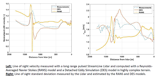
Figure 15 shows the flow model results compared to the Lidar measurements averaged for the time period 14 June 2015 1:00 p.m. to 10:30 p.m. along the Lidar beam parallel to the mean flow. The DES model is averaged over 15 FTT. Velocity estimates for both flow models are normalized by the upstream free flow velocity at 250 m from the Lidar.
The numerical results are found to predict the speed-up on the crest of the hill. However, both models predict a much higher adverse pressure gradient on the lee-side of the hill, resulting in a lower wind speed compared to the measurements. The RANS model is found to predict a full recirculation, with zero velocity at the crest of the hill. For the DES model, the largest deviations are found at approximately 1300 m from the Lidar. In the region close to the Lidar location, from approximately 0–900 m from the Lidar, the DES model provides a very good estimate for the wind speed variations along the line-of-sight. The RANS model over predicts the velocity in most of the region between the Lidar and the crest, but falls in agreement for the closest 300 m.
Figure 16 shows the measured and computational results for the one-dimensional standard deviation along the Lidar beam. The RANS model fails in predicting the variations in turbulence along the line of sight, predicting a large increase in turbulence at the peak of the crest, where both the measurements and DES-model indicates a reduction. This is expected according to theory, as wind acceleration should cause a relative reduction in turbulence at this point.
It is clear that the RANS model fails to predict the expected behavior of turbulence production and advection over the crest. The DES model provides a qualitative improvement even though the erroneous prediction of flow separation on the lee-side of the hill causes a relatively large discrepancy in the estimates.
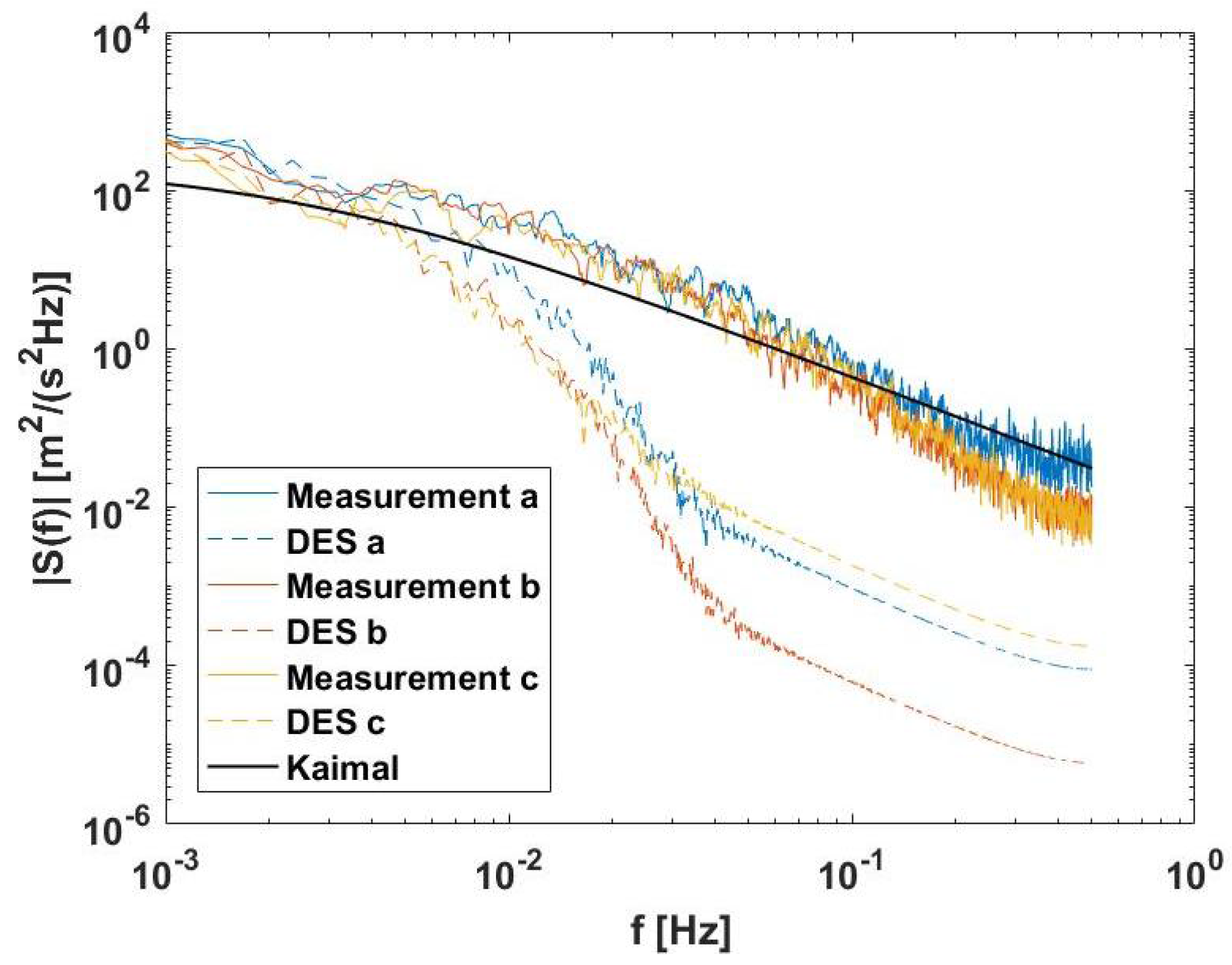
A spectral analysis was performed at three different distances from the Lidar ((a) 1000 m, (b) 600 m and (c) 400 m). The results were compared to the predicted Kaimal spectrum for the longitudinal wind based on the measured wind speed at 100 m at the measurement mast. The power density spectra for the Lidar and the DES model at the three locations are plotted in Figure 17 together with the predicted Kaimal spectrum. The RANS model is not included in this analysis as it is not a transient model.
The figure shows how the model manages to predict the low-frequency part of the spectra for all locations. There is a significant cut-off in the higher frequencies at ∼4 × 10⁻³ Hz most probably due to insufficient mesh and temporal resolution to capture the small-scale fluctuations.
For the Lidar measurements, the spectrum for location (a) has a higher power density than for location (b) and (c) for the highest frequencies. This is expected, as the measurement location is very close to the ground, where turbulence production by high shear is present.
Concerning the numerical results, the expected slope can be observed in the frequency region between 5 × 10⁻³ and 5 × 10⁻², where quantitative agreement with the measurements is achieved. For the higher frequency region (5 × 10⁻²–5 × 10⁻¹), the numerical simulation under-predicts the turbulent kinetic energy, denoting less fine flow structures are captured at all 3 positions than for the measured data. Abnormal evolutions can be seen in highest frequency region (f > 5 × 10⁻²). This denotes that the temporal resolution (time step size) is incapable of adopting the mesh resolution (cell size) applied in the simulation, and only numerical noise without any physical meaning is obtained.
The predicted Kaimal spectrum underestimates the power density for most frequencies (< Hz). The model is based on shear-introduced turbulence [18], and these results suggest that the model is not able to capture the additional mechanically induced turbulence due to the complexity of the terrain. For higher frequencies, the model is a good fit for location (a) with a higher turbulence level. Nonetheless, as the model is based on the measured speed at 100 m height, the model is not expected to be a highly accurate fit.
Note that there is a difference in the azimuth angle of 0.3° and elevation angle of ±0.2° between the measured and modeled results. The resulting deviations in the horizontal and vertical directions at the three locations along the beam are presented in Table 4.
Even though the error introduced is non-negligible, it can be disregarded considering the resolution of the mesh and the uncertainties involved in predicting the wind regime in this terrain.
4. Conclusions
In this study, the performance of a hybrid RANS/LES (DES) flow model for turbulence estimation has been evaluated by comparison with Lidar measurements in highly complex terrain.
First, the accuracy of Lidar turbulence estimates were evaluated by validation with sonic anemometer data. The analysis proved the Lidar to be very accurate in prediction of 10-min mean velocities, while the accuracy was lower for one-second measurements. This is expected, as the Lidar is affected by both spatial averaging and presence of white noise in the measurements. The possibility of increasing the accuracy of the Lidar was investigated by reducing the range gate length. With a shorter range gate length, the spatial averaging is done over a smaller volume, and the system is less affected by the spatial averaging effect. However, as the range gate is reduced, the noise level is increased, and only a slight improvement was observed when reducing the gate length from 30 m to 18 m, which is about half the FWHM scale of the Lidar. As the uncertainties related to the spatial averaging of the Lidar are relatively small compared to uncertainties in the computational model, the Lidar is assumed to be suitable for validation of flow model turbulence estimates.
The transient numerical simulation using a DES modeling strategy for turbulence estimation was tested by comparison with Lidar measurements along a beam aligned with the mean flow, pointing towards a steep ridge. This way the variation of velocity and turbulence along the beam can be determined, providing a significant improvement compared to a traditional meteorological mast measurement campaign, where only point measurements can be used for flow model validation. The DES simulation in this study overestimated the mean turbulence level somewhat, but outperformed a more traditional RANS model approach that failed to describe the turbulence behavior over the ridge.
The study shows the applicability and viability of using Lidar systems in stare mode for validating numerical models over larger distances, without a need for a significant number of point measurements. The study also shows the need for better and more reliable numerical models for predicting turbulence in highly complex terrain.
Acknowledgments
The study was funded by the ENERGIX-programme of the Research Council of Norway. We thank Statkraft AS, Meventus AS, Fraunhofer Institute for Wind Energy and Energy System Technology and the Department of Energy and Process Engineering at the Norwegian University of Science and Technology for making this research work possible.
Author Contributions
J.A.L. and Meventus conducted the experiments and collected the Lidar data used in the analysis. C.Y.C. performed the CFD simulations. A.R. performed the analysis with close help from J.A.L. and L.S. for the Lidar validation, and from C.Y.C. for the numerical analysis.
Conflicts of Interest
The authors declare no conflict of interest.
References
- Bechmann, A.; Sørensen, N.N.; Berg, J.; Mann, J.; Réthoré, P.E. The Bolund Experiment, Part II: Blind Comparison of Microscale Flow Models. Bound. Layer Meteorol. 2011, 141, 245–271. [Google Scholar] [CrossRef]
- Bechmann, A.; Sørensen, N.N. Hybrid RANS/LES Method for Wind Flow Over Complex Terrain. Wind Energy 2010, 13, 36–50. [Google Scholar] [CrossRef]
- Guillén, B.F.; Gómez, P.; Rodrigo, S.J.; Courtney, M.S.; Cuerva, A. Investigation of Sources for Lidar Uncertainty in Flat and Complex Terrain. In Proceedings of the EWEC-11, Marseille, France, 16–19 March 2009. [Google Scholar]
- Vogstad, K.; Simonsen, A.H.; Brennan, K.J.; Lund, J.A. Uncertainty of Lidars in Complex Terrain. In Proceedings of the EWEA 2013, Vienna, Austria, 4–7 February 2013. [Google Scholar]
- Lenschow, D.H.; Wulfmeyer, V. Measuring Second- Through Fourth-Order Moments in Noisy Data. J. Atmos. Ocean. Technol. 2000, 17, 1330–1347. [Google Scholar] [CrossRef]
- Bonin, T.A.; Newman, J.E.; Klein, P.M.; Chilson, P.B.; Wharton, S. Improvement of Vertical Velocity Statistics Measured by a Doppler Lidar Through Comparison With Sonic Anemometer Observations. Atmos. Meas. Tech. 2016, 9, 5833–5852. [Google Scholar] [CrossRef]
- Sjöholm, M.; Mikkelsen, T.; Mann, J.; Enevoldsen, K.; Courtney, M. Spatial Averaging-Effects on Turbulence Measured by a Continuous-Wave Coherent Lidar. Meteorol. Z. 2009, 18, 281–287. [Google Scholar] [CrossRef]
- Cañadillas, B.; Westerhellweg, A.; Neumann, T. Testing the Performance of a Ground-Based Wind LiDAR System: One Year Intercomparison at the Offshore Platform FINO1. Dewi Mag. 2011, 38, 58–64. [Google Scholar]
- Clifton, A.; Boquet, M.; Roziers, E.B.; Westerhellweg, A.; Hofsass, M.; Klaas, T.; Vogstad, K.; Clive, P.; Harris, M.; Wylie, S.; et al. Remote Sensing of Complex Flows by Doppler Wind Lidar: Issues and Preliminary Recommendations. Natl. Renew. Energy Lab. 2015. [Google Scholar] [CrossRef]
- Courtney, M.; Mann, J.; Mikkelsen, T.; Sjöholm, M. Windscanner: 3-D Wind and Turbulence Measurements from Three Steerable Doppler Lidars. In IOP Conference Series: Earth and Environmental Science (1:1); IOP Publishing: Bristol, UK, 2008. [Google Scholar]
- Fuertes, F.C.; Iungo, G.V.; Porté-Angel, F. 3D Turbulence Measurements Using Three Synchronous Wind Lidars: Validation against Sonic Anemometry. J. Atmos. Ocean. Technol. 2014. [Google Scholar] [CrossRef]
- Pearson, G.; Davies, F.; Collier, C. An Analysis of the Performance of the UFAM Pulsed Doppler Lidar for Observing the Boundary Layer. Remote Sens. 2009. [Google Scholar] [CrossRef]
- Smalikho, I.N.; Banakh, V.A. Measurements of Wind Turbulence Parameters by a Conically Scanning Coherent Doppler Lidar in the Atmospheric Boundary Layer. Atmos. Meas. Tech. 2017, 10, 4191–4208. [Google Scholar] [CrossRef]
- Walpole, R.E.; Ye, K.; Myers, S.L.; Myers, R.H. Probability and Statistics for Engineers and Scientists, 8th ed.; Pearson Education International: Upper Saddle River, NJ, USA, 2007. [Google Scholar]
- Pope, S.B. Turbulent Flows; Cornell University: Ithaca, NY, USA, 2000; pp. 182–191. [Google Scholar]
- Monin, A.S.; Obukhov, A.M. Basic Laws of Turbulent Mixing in the Surface Layer of the Atmosphere. Tr. Akad. Nauk SSSR Geophiz. Inst. 1954, 24, 163–187. [Google Scholar]
- Spalart, P.R. Strategies for Turbulence Modelling and Simulations. Int. J. Heat Fluid Flow 2000, 21, 252–263. [Google Scholar] [CrossRef]
- Kaimal, J.; Wyngaard, J.; Izumi, Y.; Coté, O. Spectral Characteristics of Surface-Layer Turbulence. Q. J. R. Meteorol. Soc. 1972, 98, 563–589. [Google Scholar] [CrossRef]
- Beaupuits, J.P.P.; Otárola, A.; Rantakyrö, F.; Rivera, R.; Radford, S.; Nyman, L. Analysis of Wind Data Gathered at Chajnantor; ALMA Memo: Charlottesville, VA, USA, 2004; Volume 497. [Google Scholar]
- Weir, D.E. Vindkraft—Produksjon i 2013; Norges Vassdrags- og Energidirektorat: Oslo, Norway, 2014. [Google Scholar]
- Quaas, J.; Stevens, B.; Stier, P.; Lohmann, U. Interpreting the Cloud Cover—Aerosol Optical Depth Relationship Found in Satellite Data Using a General Circulation Model. Atmos. Chem. Phys. 2010, 10, 6129–6135. [Google Scholar] [CrossRef]
- Sathe, A.; Mann, J.; Gottschall, J.; Courtney, M. Can Wind Lidars Measure Turbulence? J. Atmos. Ocean. Technol. 2011, 28, 853–868. [Google Scholar] [CrossRef]
Figure 1.
Map of the site with the position of the Lidar (64°08′20.7″ N 10°19′04.0″ E) and the meteorological mast (64°08′09.7″ N 10°19′00.7″ E). The height contours represent 5 m height difference.
Figure 1.
Map of the site with the position of the Lidar (64°08′20.7″ N 10°19′04.0″ E) and the meteorological mast (64°08′09.7″ N 10°19′00.7″ E). The height contours represent 5 m height difference.
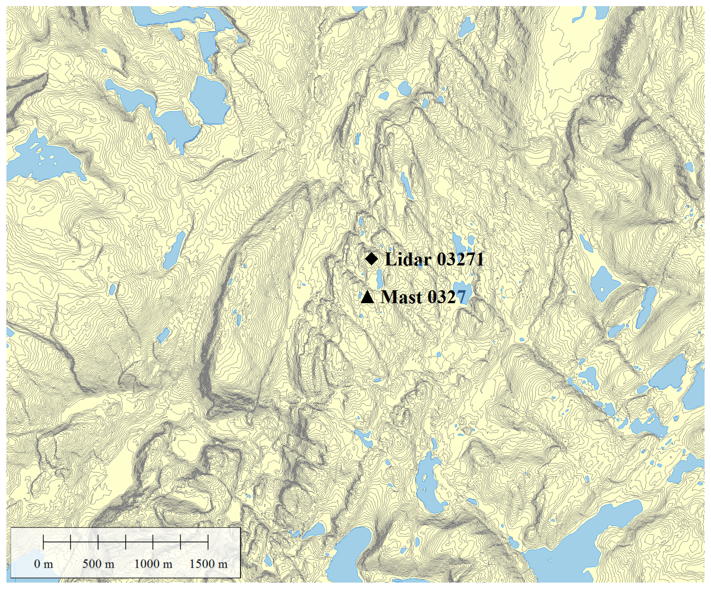
Figure 2.
Schematic of the Lidar and mast positions. Left: side view of the setup. The elevation angle is 15.26°; Right: top view of the setup. Azimuth angle = 180° + a, a = 6.86°. To avoid backscatter from the sonic anemometer, the Lidar azimuth was set to 186.94°, pointing approximately 0.5 m west of the sonic anemometer. The sonic anemometer is mounted on a 5 m long boom at an angle b = 45°.

Figure 3.
Wind velocity and direction during 30 April 2015 measured by the sonic anemometer. Times are local (UTC + 1:00).
Figure 3.
Wind velocity and direction during 30 April 2015 measured by the sonic anemometer. Times are local (UTC + 1:00).
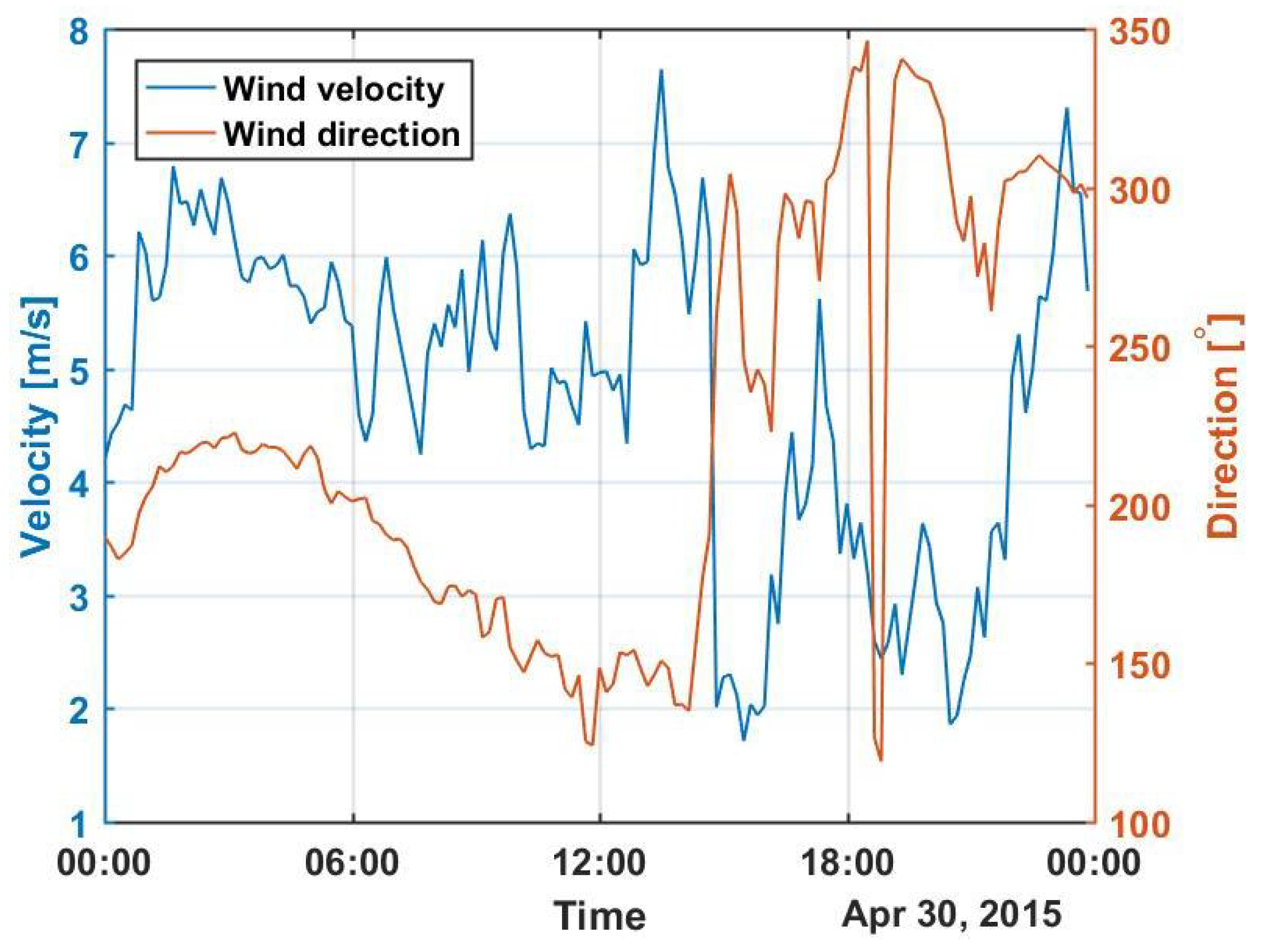
Figure 4.
Schematic describing the location of the Lidar and meteorological mast, and the ridge of interest to the study. Flow model results were compared with Lidar measurements along the line-of-sight parallel to the mean flow, and points at distances (a) 1000 m; (b) 600 m; and (c) 400 m from the Lidar were used for further evaluations.

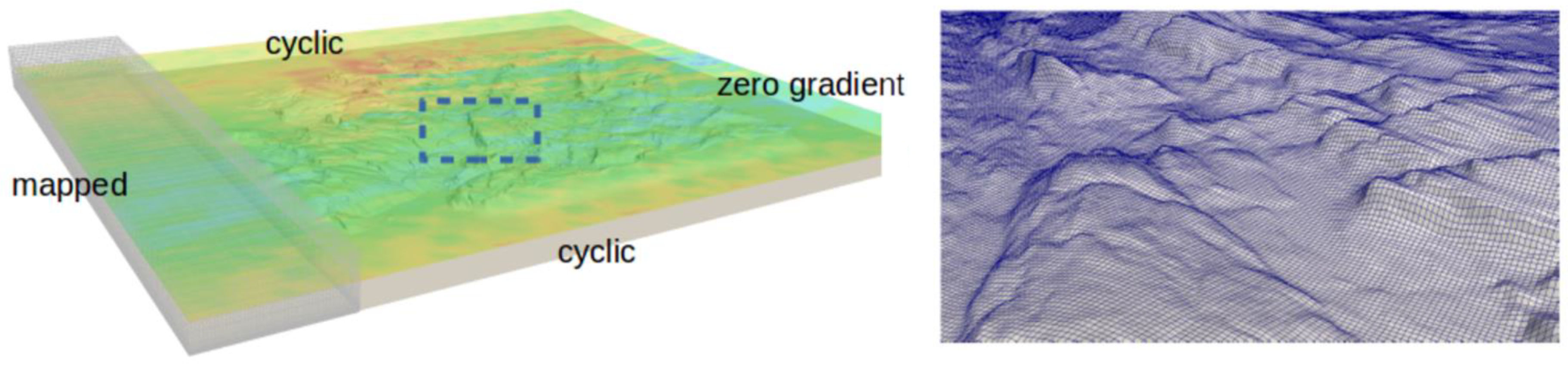
Figure 5.
Right: illustration of the computational domain with the prolonged inlet. The boundary conditions used in the simulation are illustrated. The ridge of interest can be seen in the center of the domain. The color coding represent velocity magnitude; Left: close up of the structured grid at the ridge.

Figure 6.
Coefficient of determination R2 and availability versus the lower Signal-to-noise ratio (SNR) limit.
Figure 6.
Coefficient of determination R2 and availability versus the lower Signal-to-noise ratio (SNR) limit.
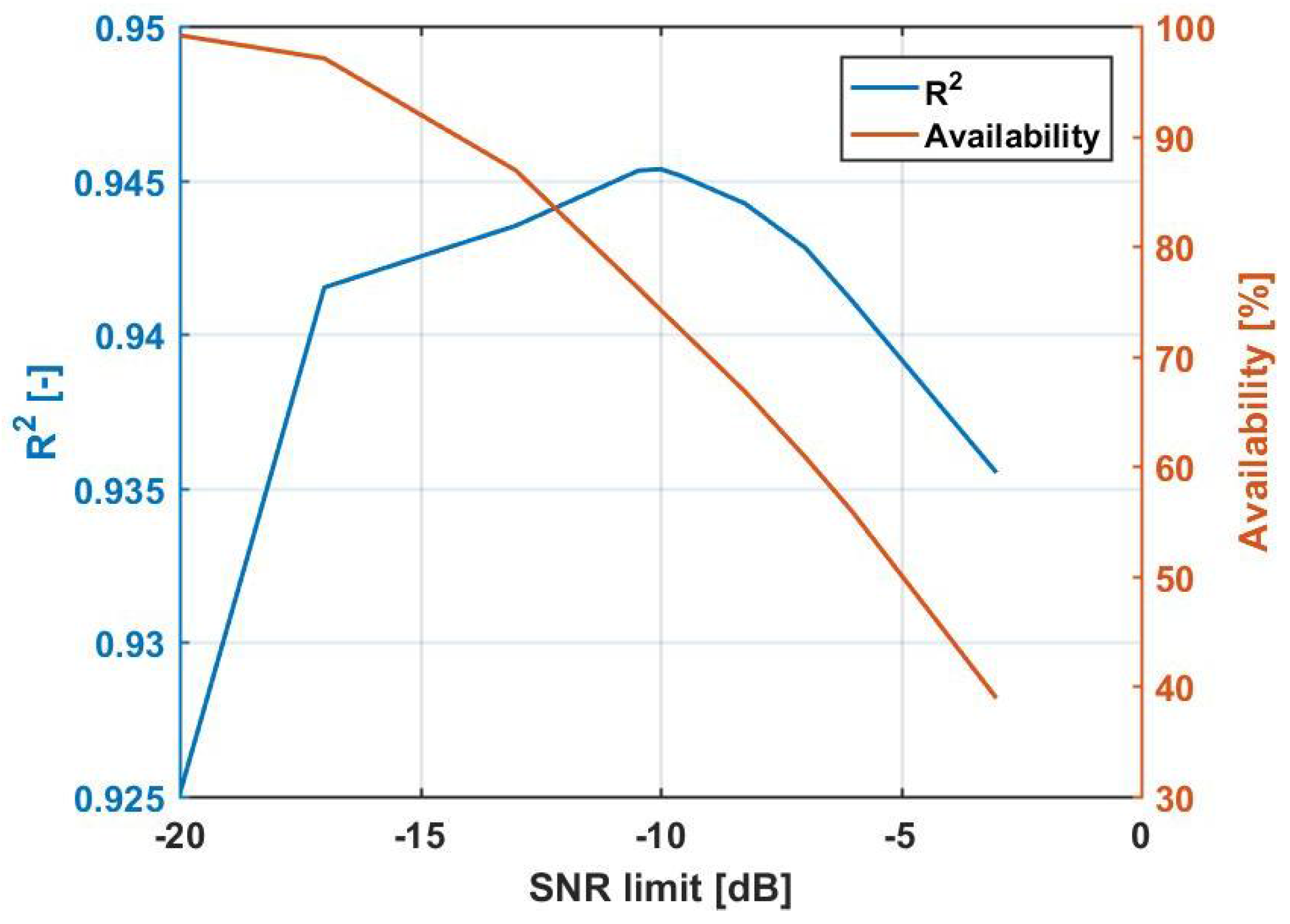
Figure 7.
Temperature, relative humidity and SNR versus time for a 24 h period on 30 April 2015. The optimal SNR limit of −10 dB is included as a reference. Times are local (UTC+1:00).
Figure 7.
Temperature, relative humidity and SNR versus time for a 24 h period on 30 April 2015. The optimal SNR limit of −10 dB is included as a reference. Times are local (UTC+1:00).
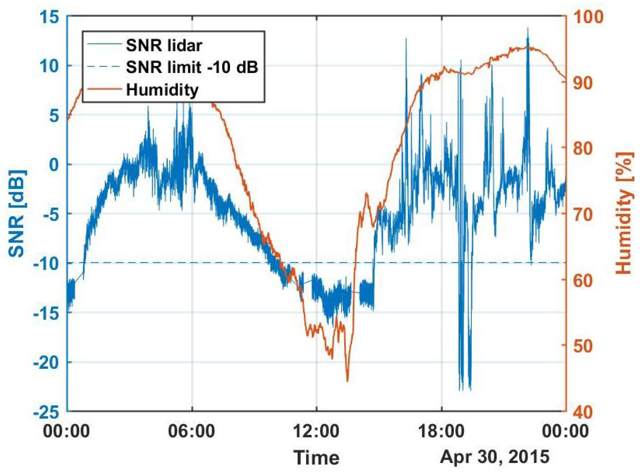
Figure 8.
Time series of one-dimensional 1 Hz velocities from 13 April 2015–11 June 2015 measured with the Lidar and the sonic anemometer. Times are local (UTC + 1:00).
Figure 8.
Time series of one-dimensional 1 Hz velocities from 13 April 2015–11 June 2015 measured with the Lidar and the sonic anemometer. Times are local (UTC + 1:00).
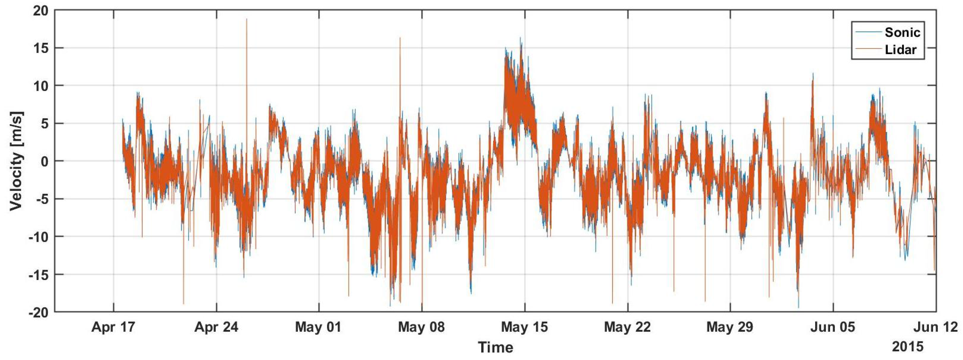
Figure 9.
Correlation plot of ten-minute averaged velocities from 13 April 2015–11 June 2015. The coefficient of determination is R2 = 0.9972 and the linear regression slope is 1.0043.
Figure 9.
Correlation plot of ten-minute averaged velocities from 13 April 2015–11 June 2015. The coefficient of determination is R2 = 0.9972 and the linear regression slope is 1.0043.
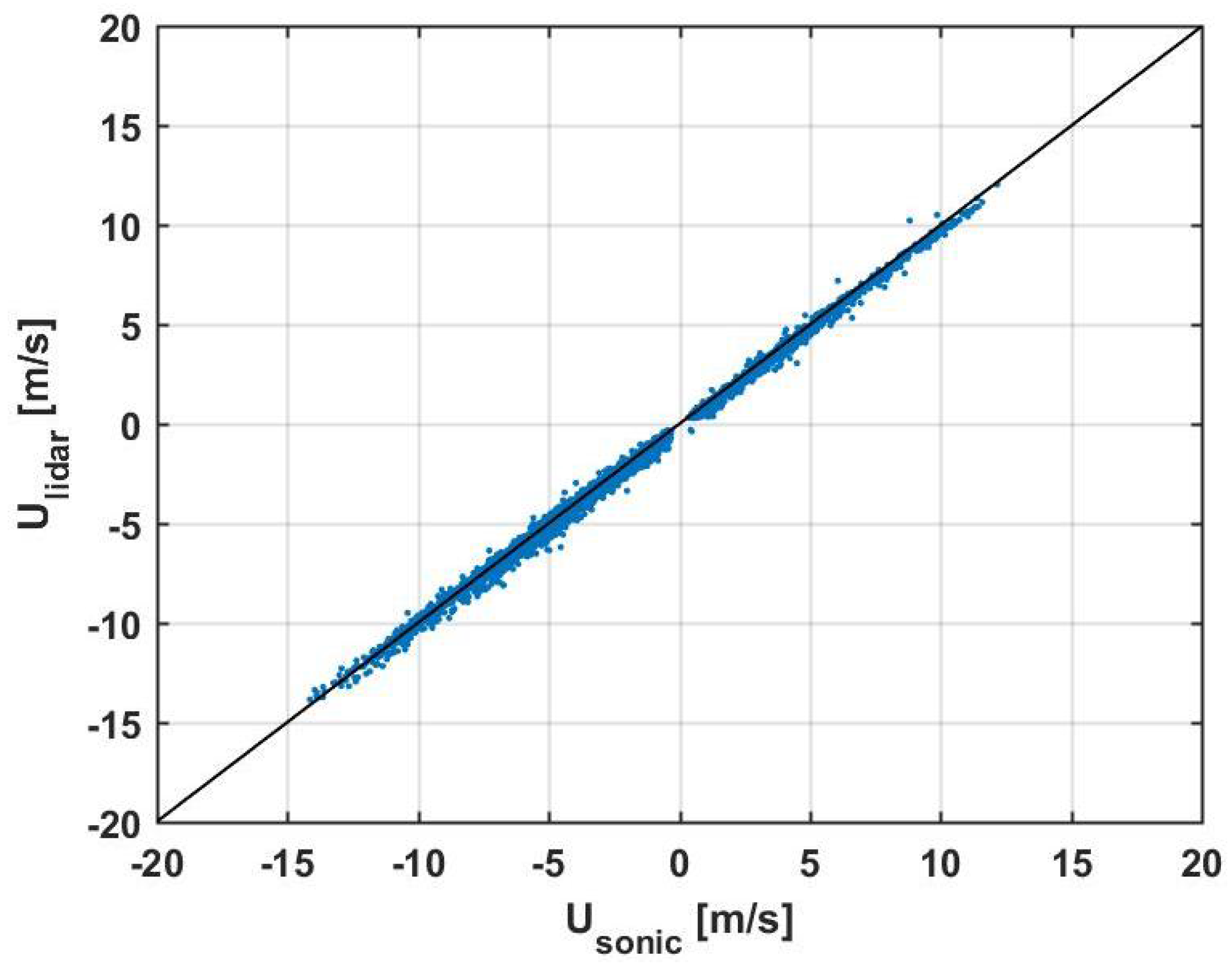
Figure 10.
Correlation plot of one-second velocities from 13 April 2015–11 June 2015. The coefficient of determination is R2 = 0.9454 and the linear regression slope is 0.9705.
Figure 10.
Correlation plot of one-second velocities from 13 April 2015–11 June 2015. The coefficient of determination is R2 = 0.9454 and the linear regression slope is 0.9705.
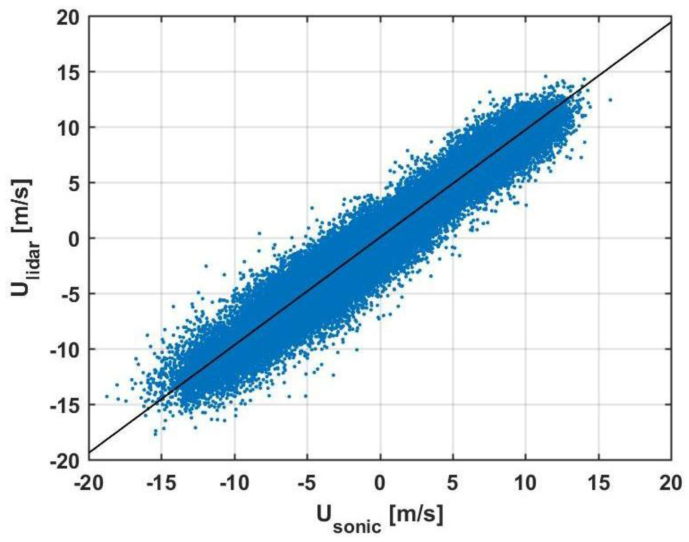
Figure 11.
Ten-minute mean turbulence intensity versus velocity for the Lidar and the sonic anemometer.
Figure 11.
Ten-minute mean turbulence intensity versus velocity for the Lidar and the sonic anemometer.
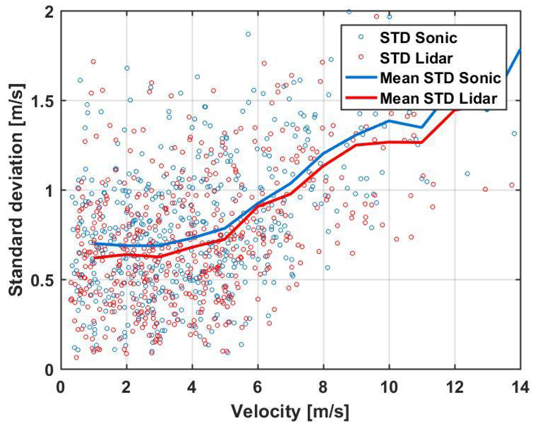
Figure 12.
Power density spectra for the Lidar and the sonic anemometer, and the theoretical Kolmogorov slope.
Figure 12.
Power density spectra for the Lidar and the sonic anemometer, and the theoretical Kolmogorov slope.

Figure 13.
Coefficient of determination versus lower SNR limit for the three different range gate lengths on 30 April 2015.
Figure 13.
Coefficient of determination versus lower SNR limit for the three different range gate lengths on 30 April 2015.

Figure 14.
Power density spectra for the Lidar with different range gate lengths, the sonic anemometer and the theoretical Kolmogorov slope.
Figure 14.
Power density spectra for the Lidar with different range gate lengths, the sonic anemometer and the theoretical Kolmogorov slope.
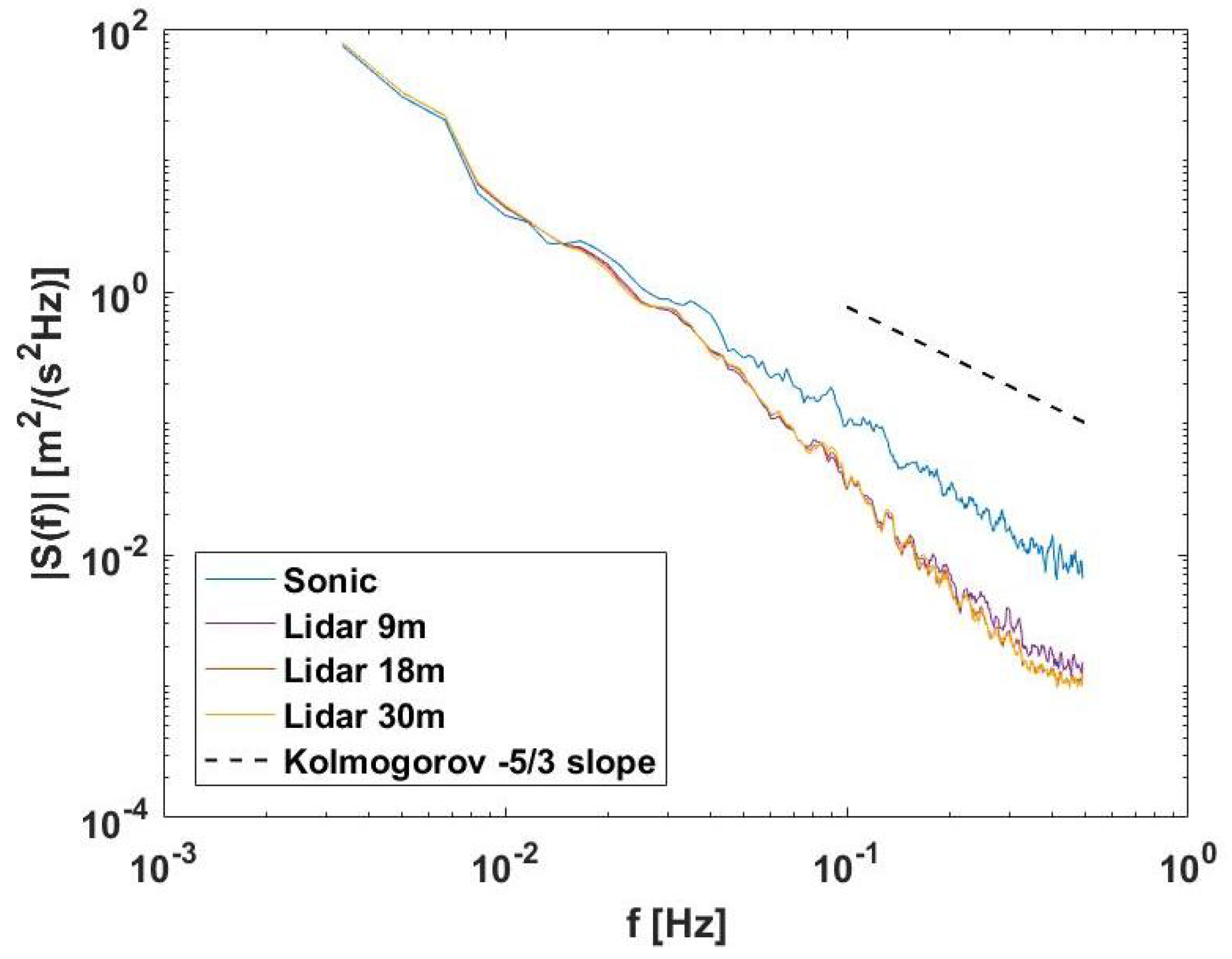
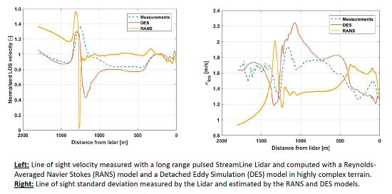
Figure 15.
Velocity along the Lidar beam normalized by the upstream free flow velocity averaged for 14 June 2015 1:00 p.m. to 10:30 p.m. measured by the Lidar and computed with the Reynolds-Averaged Navier-Stokes (RANS) and Detached Eddy Simulation (DES) model.
Figure 15.
Velocity along the Lidar beam normalized by the upstream free flow velocity averaged for 14 June 2015 1:00 p.m. to 10:30 p.m. measured by the Lidar and computed with the Reynolds-Averaged Navier-Stokes (RANS) and Detached Eddy Simulation (DES) model.
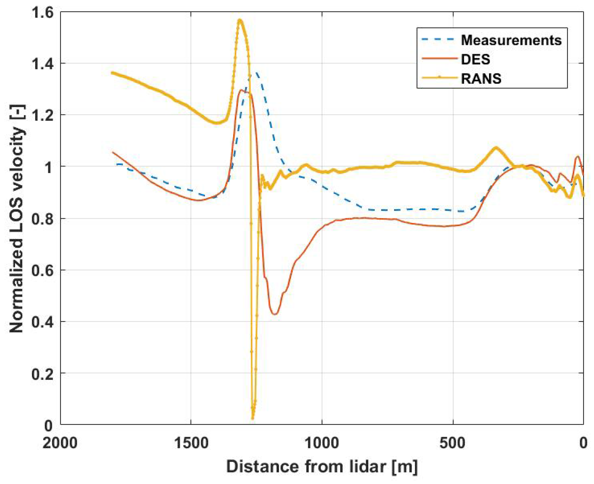
Figure 16.
Standard deviation along the Lidar beam averaged for 14 June 2015 1:00 p.m. to 10:30 p.m. estimated by the Lidar and computed with the RANS and DES model.
Figure 16.
Standard deviation along the Lidar beam averaged for 14 June 2015 1:00 p.m. to 10:30 p.m. estimated by the Lidar and computed with the RANS and DES model.
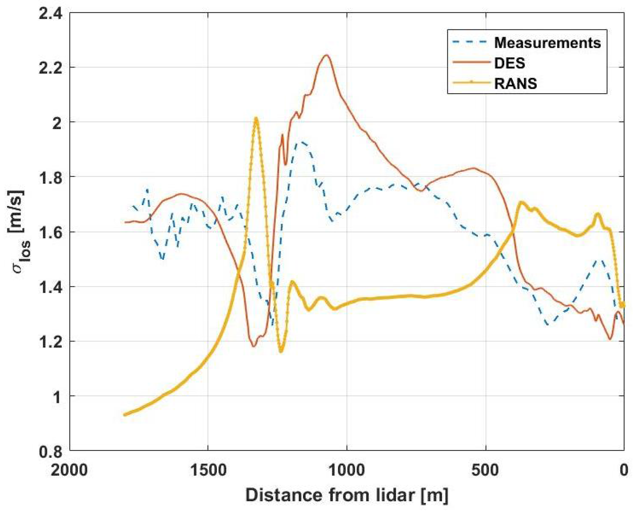
Figure 17.
Power density spectra for the Lidar and the DES model at distances (a) 1000 m, (b) 600 m and (c) 400 m from the Lidar, and the estimated Kaimal spectrum during 14 June 2015 1:00 p.m. to 10:30 p.m.
Figure 17.
Power density spectra for the Lidar and the DES model at distances (a) 1000 m, (b) 600 m and (c) 400 m from the Lidar, and the estimated Kaimal spectrum during 14 June 2015 1:00 p.m. to 10:30 p.m.

Table 1.
Instrumentation installed on the measurement mast. All cup anemometers are mounted on booms pointing southwest from the mast. At 100.5 m height, there is an additional cup anemometer on a boom pointing northeast.
Table 1.
Instrumentation installed on the measurement mast. All cup anemometers are mounted on booms pointing southwest from the mast. At 100.5 m height, there is an additional cup anemometer on a boom pointing northeast.
| Parameter | Type | Height (m) | Boom Direction (°) from Mast | Boom Length (m) |
|---|---|---|---|---|
| Wind speed | Thies First ClassAdvanced | 100.5 | 225 | 1.015 |
| Wind speed | Thies First ClassAdvanced | 100.5 | 45 | 1.015 |
| Wind speed | Thies First ClassAdvanced | 80.0 | 225 | 5.028 |
| Wind speed | Thies First ClassAdvanced | 60.0 | 225 | 5.028 |
| Wind speed | Thies First ClassAdvanced | 40.0 | 225 | 5.028 |
| Wind speed | Thies First ClassAdvanced | 20.7 | 225 | 5.028 |
| Wind speed | 3D UltrasonicThies | 98.0 | 225 | 5.028 |
| Wind direction | 3D UltrasonicThies | 98.0 | 225 | 5.028 |
| Temperature | 3D UltrasonicThies | 98.0 | 225 | 5.028 |
| Vertical wind speed | 3D UltrasonicThies | 98.0 | 225 | 5.028 |
| Wind direction | Thies First ClassTMR | 98.0 | 44 | 5.028 |
| Wind direction | Thies First ClassTMR | 40.0 | 44 | 5.028 |
| Wind direction | NRG IceFree3 | 80.0 | 42 | 5.028 |
| Temperature | Galltec Mess KP | 97.0 | 20 | 0.305 |
| Relative humidity | Galltec Mess KP | 97.0 | 20 | 0.305 |
| Temperature | Galltec Mess TP | 3.0 | 20 | 0.305 |
| Barometric pressure | Ammonit AB 60 | 3.0 | - | - |
| Aviation lights | ObeluxLI-32+IR-DCW-F | 97.6 | - | - |
Table 2.
Wind conditions observed during the selected time period. Times are local (UTC + 1:00).
| Time Period | Wind Speed @100 m Mean (min, max) (m/s) | Wind Direction @100 m Mean (min, max) (°) | Monin–Obhukov Length Scale (min) (m) |
|---|---|---|---|
| 14 June 2015 1:00 p.m. to 10:30 p.m. | 8.3 (7, 10) | 260 (250, 290) | (450) |
Table 3.
Optimal R2 values and the corresponding Signal-to-noise ratio (SNR) limit and availability for the different range gate lengths.
Table 3.
Optimal R2 values and the corresponding Signal-to-noise ratio (SNR) limit and availability for the different range gate lengths.
| Range Gate Length (m) | Opt. R2 (-) | Opt. SNR Limit (dB) | Availability (%) |
|---|---|---|---|
| 9 | 0.9657 | −4.44 | 55.4 |
| 18 | 0.9657 | −4.69 | 57.2 |
| 30 | 0.9650 | −4.95 | 58.0 |
Table 4.
Horizontal and vertical deviations at the three locations along the beam caused by the difference in azimuth and elevation angle between the measured and modeled results.
Table 4.
Horizontal and vertical deviations at the three locations along the beam caused by the difference in azimuth and elevation angle between the measured and modeled results.
| Location | Horizontal Deviation (m) | Vertical Deviation (m) |
|---|---|---|
| (a) | 5.2 | 3.5 |
| (b) | 3.1 | 2.1 |
| (c) | 2.1 | 1.4 |
© 2018 by the authors. Licensee MDPI, Basel, Switzerland. This article is an open access article distributed under the terms and conditions of the Creative Commons Attribution (CC BY) license (http://creativecommons.org/licenses/by/4.0/).
Share and Cite
MDPI and ACS Style
Risan, A.; Lund, J.A.; Chang, C.-Y.; Sætran, L. Wind in Complex Terrain—Lidar Measurements for Evaluation of CFD Simulations. Remote Sens. 2018, 10, 59. https://doi.org/10.3390/rs10010059
AMA Style
Risan A, Lund JA, Chang C-Y, Sætran L. Wind in Complex Terrain—Lidar Measurements for Evaluation of CFD Simulations. Remote Sensing. 2018; 10(1):59. https://doi.org/10.3390/rs10010059
Chicago/Turabian StyleRisan, Andrea, John Amund Lund, Chi-Yao Chang, and Lars Sætran. 2018. "Wind in Complex Terrain—Lidar Measurements for Evaluation of CFD Simulations" Remote Sensing 10, no. 1: 59. https://doi.org/10.3390/rs10010059
Note that from the first issue of 2016, this journal uses article numbers instead of page numbers. See further details here.