The Impact of Lidar Elevation Uncertainty on Mapping Intertidal Habitats on Barrier Islands
by
 , , ,
, , ,
Nicholas M. Enwright
1,2,* ,
,
Lei Wang
2,
Sinéad M. Borchert
3,
Richard H. Day
1,
Laura C. Feher
1 and
Michael J. Osland
1 1
Wetland and Aquatic Research Center, U.S. Geological Survey, Lafayette, LA 70506, USA
2
Department of Geography and Anthropology, Louisiana State University, Baton Rouge, LA 70803, USA
3
Borchert Consulting at the Wetland and Aquatic Research Center, U.S. Geological Survey, Lafayette, LA 70506, USA
*
Author to whom correspondence should be addressed.
Remote Sens. 2018, 10(1), 5; https://doi.org/10.3390/rs10010005
Submission received: 16 November 2017
/
Revised: 13 December 2017
/
Accepted: 15 December 2017
/
Published: 21 December 2017
(This article belongs to the Special Issue Uncertainty in Remote Sensing Image Analysis)
Abstract
:While airborne lidar data have revolutionized the spatial resolution that elevations can be realized, data limitations are often magnified in coastal settings. Researchers have found that airborne lidar can have a vertical error as high as 60 cm in densely vegetated intertidal areas. The uncertainty of digital elevation models is often left unaddressed; however, in low-relief environments, such as barrier islands, centimeter differences in elevation can affect exposure to physically demanding abiotic conditions, which greatly influence ecosystem structure and function. In this study, we used airborne lidar elevation data, in situ elevation observations, lidar metadata, and tide gauge information to delineate low-lying lands and the intertidal wetlands on Dauphin Island, a barrier island along the coast of Alabama, USA. We compared three different elevation error treatments, which included leaving error untreated and treatments that used Monte Carlo simulations to incorporate elevation vertical uncertainty using general information from lidar metadata and site-specific Real-Time Kinematic Global Position System data, respectively. To aid researchers in instances where limited information is available for error propagation, we conducted a sensitivity test to assess the effect of minor changes to error and bias. Treatment of error with site-specific observations produced the fewest omission errors, although the treatment using the lidar metadata had the most well-balanced results. The percent coverage of intertidal wetlands was increased by up to 80% when treating the vertical error of the digital elevation models. Based on the results from the sensitivity analysis, it could be reasonable to use error and positive bias values from literature for similar environments, conditions, and lidar acquisition characteristics in the event that collection of site-specific data is not feasible and information in the lidar metadata is insufficient. The methodology presented in this study should increase efficiency and enhance results for habitat mapping and analyses in dynamic, low-relief coastal environments.
1. Introduction
Barrier islands are subaerial expressions consisting of wave-, wind-, and/or tide-deposited sediments found along portions of coasts on every continent except Antarctica [1,2]. Due to their position along the land-sea interface, barrier islands often experience rapid episodic impacts related to storms as well as gradual changes related to anthropogenic activity, tides, and currents. Thus, natural resource managers are concerned with monitoring the extent and condition of these important coastal environments over time [3]. Remote sensing provides an important tool for monitoring the dynamic nature of barrier island systems [4,5].
Barrier islands provide numerous ecosystem services, including storm protection and erosion control to the mainland, habitat for fish and wildlife, salinity regulation in estuaries, carbon sequestration in marshes, water catchment and purification, recreation, and tourism [6]. Intertidal wetlands, which make up a substantial proportion of area on barrier islands, include areas that are regularly exposed to saline waters via high tides and areas that are periodically exposed to saline waters via extreme spring tides [7]. Though difficult to value, these wetlands support ecosystem goods and services that are estimated to be worth U.S. $194,000 per hectare per year [8]. In addition to providing fish and wildlife habitat, tidal wetlands can improve water quality, ameliorate flooding impacts, support coastal food webs, and protect coastlines [6]. Detailed wetland habitat mapping, such as the maps produced via the U.S. Fish and Wildlife National Wetlands Inventory Program, have commonly been developed using approaches that rely heavily on expert manual photointerpretation [9] and sometimes use elevation data as a guide [10]. Elevation information has also been combined with aerial photography for several habitat mapping efforts specific to barrier islands [11,12,13]. For example, McCarthy and Halls [12] mapped barrier island habitats in North Carolina and used elevation data to delineate habitats based on tidal regimes (e.g., intertidal and supratidal).
While lidar technology has led to advancements in coastal wetland habitat mapping methodologies [14], lidar vertical errors can often present unique challenges for lidar applications in these low-slope environments. Lidar vertical error commonly varies by land cover type [15], and vegetation cover has been found to be one of the greatest sources of error in lidar data [16]. The level of uncertainty from data collected with conventional aerial linear lidar systems is considerable within intertidal areas and can be as high as 60 cm in densely vegetated emergent wetlands [17,18]. Researchers have grappled with the challenges related to gauging the vertical error of lidar in intertidal areas and developing approaches to deal with these issues. These approaches have ranged from simple techniques, such as using a minimum bin approach [19], to more complex regression-based corrections that relate biomass estimation to the relative accuracy of digital elevation models (DEMs) estimated from Real-Time Kinematic Global Position System (RTK GPS) observations [17,18]. Due to the lack of detailed error information, the uncertainty of DEMs is often left unaddressed for habitat mapping efforts, yet the level of uncertainty becomes critical when studying low-relief environments where centimeters can make a difference in the exposure to physically demanding abiotic conditions (e.g., inundation, salt spray, wave energy) [20,21]. In the near future, advancements in lidar technology, such as single photon and Geiger-mode lidar sensors [22] and unmanned aerial system (UAS) lidar data collection [23,24] should lead to higher frequency of high-quality elevation data for use by scientists and natural resource managers. As more and more data become available, one question that may arise for scientists is how to best leverage these data to produce automated inventories of elevation-dependent habitats in coastal environments for detailed monitoring of habitat changes over time.
One classic approach for dealing with vertical error in DEMs is through the use of Monte Carlo simulations [25,26]. For example, one simple application of Monte Carlo simulations is to propagate error and determine the probability that the elevation is below a specific threshold for a set of iterations. This approach has become a popular way to incorporate vertical uncertainty in sea-level rise modeling applications [27,28]. Liu et al. used Monte Carlo simulations and error reported from lidar metadata to delineate the mean high water shoreline on the Bolivar Peninsula in Texas, USA [29]. Our work builds on this approach to extend the automated delineation to the full intertidal zone. In doing so, it is important to be sure that the error estimate incorporates vegetated land cover types and represents the 95th percentile error, since error commonly deviates from a normal distribution in vegetated land cover types [30]. Furthermore, the utilization of a bias constraint in the Monte Carlo analyses [26] becomes critical as the intertidal boundary often extends into densely vegetated areas, which tend to lead to overestimation of elevation.
The primary objective of this study was to apply a simple approach to enhance results of automated intertidal area mapping using lidar data. We used tide gauge information, site-specific RTK GPS data, and information from a detailed relative accuracy report (i.e., lidar metadata) that followed the American Society of Photogrammetry and Remote Sensing’s (ASPRS) standards [30] to simulate the propagation of elevation uncertainty into a lidar-based DEM using Monte Carlo simulations. We compared three different elevation error treatments, which included leaving error untreated and treatments that used Monte Carlo simulations to incorporate elevation vertical uncertainty using general information from lidar metadata and site-specific RTK GPS data, respectively. For each of the error treatments, we assessed the effect of error handling on automated delineation of low-lying lands (i.e., low-lying lands below the extreme high water spring (EHWS) tidal datum) and the delineation of the intertidal wetlands (Figure 1). In some cases, the collection of site-specific RTK GPS data may not be feasible and detailed metadata information with a relative elevation accuracy assessment specific to vegetated low-lying land cover types may not be available. In these instances, researchers may opt to use information identified in literature from similar environments, specifically with regards to vegetation community. To aid researchers facing this predicament, we conducted a sensitivity test to explore how estimates of low-lying areas could be influenced by changes to error and bias. In this study, we investigated the following research questions: (1) How does extraction of low-lying lands compare for the three elevation error treatments in terms of areal coverage and accuracy? (2) How does the extraction of intertidal wetlands compare for the three elevation error treatments in terms of areal coverage? (3) How sensitive are error and bias parameters for the identification of low-lying lands?
2. Materials and Methods
2.1. Study Site
Dauphin Island (Alabama, USA) is a barrier island with a length of about 25 km, from about −88.34° to −88.07° longitude. At the widest point, the island extends from about 30.28° to 30.23° latitude (Figure 2). In December of 2015, the island had a subaerial area of about 13.6 km2 [31]. The barrier island comprises a portion of a 105-km long Mississippi–Alabama wave-dominated barrier island chain that is backed by the shallow (<4-m depth) Mississippi Sound [32]. A tide gauge, first established in 1966 and operated by the National Oceanic and Atmospheric Administration (NOAA) (station ID: 8735180), is located on the eastern side of the island (Figure 2). The island is a microtidal environment, and experiences diurnal tides with a mean range of tide of about 0.36 m (i.e., height difference between mean low water and mean high water tidal datums), based on observations from the NOAA tide gauge on the island during the most recent North American Tidal Datum Epoch (NTDE; 1983 to 2001). The maximum observed water level at this gauge was about 2.01 m above mean sea level, which occurred during Hurricane Katrina in 2005. Numerous impacts from hurricanes have been documented on Dauphin Island with the most recent impacts occurring during Hurricane Katrina [33].
2.2. Elevation Data
We used aerial topographic linear lidar acquired during January 2015 by Digital Aerial Solutions, LLC (DAS; Riverview, FL, USA) and the U.S. Geological Survey (USGS). The lidar data were collected with the Leica ALS70 and ALS80 sensors. This data collection occurred over an extensive area (5400 km2) that included barrier islands in Alabama, Mississippi, and part of Louisiana. The acquisition area included 184 survey lines and 21 control lines positioned to have a nominal side overlap of 30%. These data were collected at an altitude of about 1800 m and a ground speed of 155 knots. The laser rate was 132 kHz and the scan rate was 66.2 Hz. Airborne and ground GPS observations were collected at a frequency of 2 Hz and inertial measurement unit observations were collected at 200 Hz. These data were collected with a nominal pulse density of about 6 points per m2 and adhered to the USGS quality level 2 standards [34]. A 1-m DEM, which was used for this effort, was developed to support the USGS 3D Elevation Program (3DEP) [35] by DAS and the USGS. See Heidemann et al. [34] for information on USGS standards for lidar acquisition and Arundel et al. [36] for information on 1-m DEM development. The vertical datum of the data was the North American Vertical Datum of 1988 (NAVD88) GEOID 12a.
2.3. Tide and Water Level Data
We used tidal datum data from the NOAA Dauphin Island tide gauge (Figure 2). For this gauge, the mean sea level (MSL) was estimated to be 0.018 m higher than NAVD88 for the observations during the most recent NTDE. We transformed the vertical datum of the DEMs to MSL by adding this relative height difference to the DEM. Esri ArcMap 10.4.1 (Redlands, CA, USA) was used for all spatial analyses.
Intertidal wetlands fall above the extreme low water spring and below the EHWS tidal datums [7]. We defined EHWS as the highest astronomical tide predicted for the Dauphin Island tide gauge (0.448 m relative to MSL), which is the highest predicted water level under astronomical conditions alone during the most recent NTDE.
2.4. Field Data Collection
We collected field data over two and a half weeks in November and December of 2015. Elevation data were collected using a high-precision RTK GPS connected to a Global Navigation Satellite System (GNSS) (Trimble R10 and TSC3, Trimble, Sunnyvale, CA, USA), coupled with the Continuously Operating Reference Station (CORS) network for Mississippi and Alabama (University of Southern Mississippi’s network and Alabama Department of Transportation’s CORS, respectively). The estimated precision from RTK GPS observations was about ±0.04 m (mean = 0.039, median = 0.037, interquartile range = 0.021). The habitat type was observed for each elevation observation. These observations were collected via cluster sampling to support a habitat mapping effort [31]. Site accessibility related to private land was one of the main factors in the spatial distribution of the points. For more information on field data collection, see Enwright et al. [31].
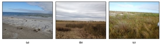
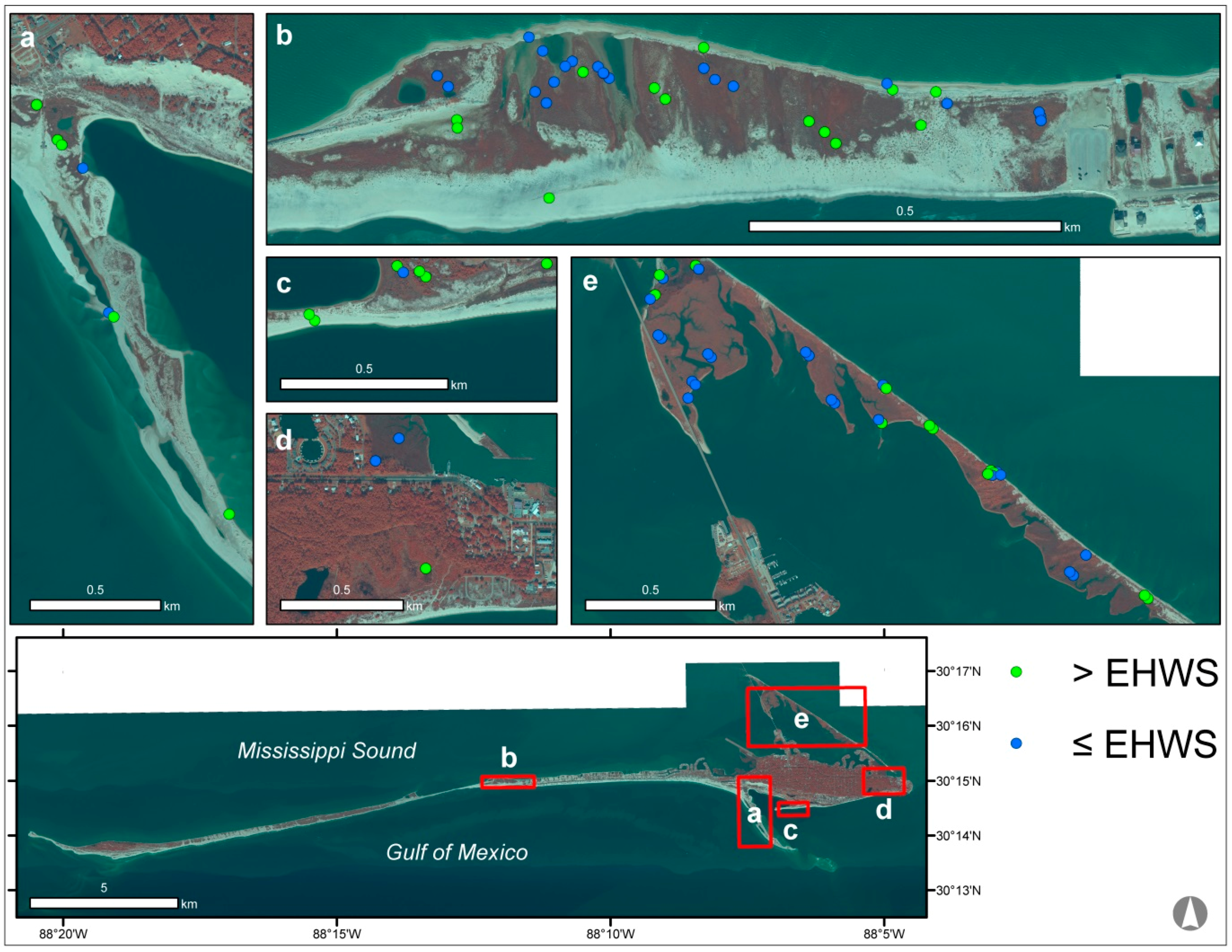
For this study, we created two subsets from the RTK GPS points. The first subset was used to conduct a relative accuracy assessment between the site-specific RTK GPS points and the 1-m DEM. A total of 62 points were collected in three different habitats which included intertidal flat (n = 7; Figure 3a), intertidal emergent marsh (n = 29; Figure 3b), and meadow (n = 26; Figure 3c). Meadows are supratidal areas with emergent herbaceous vegetation similar to wetlands found on the backslopes of the back-barrier. The second subset of the RTK GPS points was used to validate the results for identifying low-lying lands. We used datum information from the NOAA Dauphin Island tide gauge to transform the RTK GPS elevations to MSL. We restricted the subset to include points from any habitat that were below the elevation of 0.936 m (i.e., double the elevation of EHWS + 0.04 m; n = 86). A binary variable was created for these observations for which points with an elevation that was less than or equal to 0.488 m (EHWS + 0.04 m) were coded to “1” (n = 48) and those with an elevation greater than 0.488 m were coded to “0” (n = 38).
2.5. Error and Bias
Propagation of lidar data vertical uncertainty by using Monte Carlo simulations requires an estimate of lidar DEM error and, if relevant, bias. We developed two different relative vertical error and bias estimates by comparing elevation collected via RTK GPS with the 1-m lidar DEM. The site-specific RTK GPS sample (n = 62) was right-skewed (i.e., skewness = 0.545) with a 95th percentile value of 0.415 m and a positive bias for 76% of the observations (Table 1). Based on the RTK GPS precision analyses, we assumed that points that were within ±0.04 m were not different for determining the percentage of observations with a positive bias (the DEM observation is higher than RTK GPS observation). Note, the bias identified in this study was similar to the bias found in a similar study in coastal wetlands by Buffington et al. [18]. The second error and bias estimate was based on information reported in the metadata for the lidar DEM product. These data came from RTK GPS observations throughout the extensive lidar acquisition extent from areas classified as either open, nonvegetated terrain, tall weed, brush land, forest, or urban. To make this analysis comparable to the site-specific analysis, we only used points from the open, nonvegetated terrain (n = 22) and tall weed (n = 18) classes that fell below 1 m relative to NAVD88. The pooled sample (n = 40) was right-skewed (i.e., skewness = 0.959) with a 95th percentile value of 0.326 m and a positive bias for 54% of the observations (Table 1). For both vertical error assessments, the bias for nonvegetated and vegetated areas were combined to develop a simple average bias value which was rounded to nearest integer. SigmaPlot 12.5 (Systat Software, Inc., San Jose, CA, USA) was used for all nonspatial statistical analyses in this study, unless otherwise noted.
2.6. Monte Carlo DEM Error Propagation
Monte Carlo analyses provide an efficient way to simulate the propagation of vertical error into DEMs for coastal applications involving tidal datums and sea-level rise [37]. In this study, error propagation followed an approach similar to that of Cooper and Chen [37], with the addition of enhancements such as a neighborhood spatial autocorrelation filter and bias constraint used by Wechsler and Kroll [26].
Figure 4 shows a general overview of the Monte Carlo simulation process used in this study. The first step in the error propagation was the development of a random field. In our case, we used a raster with a normal distribution with a mean of 0 and a standard deviation of 0.5. We forced the bias to be either positive or negative for each random field, collectively based on the proportional positive bias identified in the relative elevation analyses (Table 1). Next, a local filter (a 3-by-3-pixel neighborhood) was used to incorporate spatial autocorrelation into the simulated random fields [26]. The filtered raster was multiplied by the 95th percentile error (Table 1) and added to the original DEM. The use of the 95th percentile error is recommended by the ASPRS when dealing with vertical error for areas that include vegetated areas [30]. The result of adding the product of the 95th percentile error and the random field to the DEM is the simulation of the propagation of error into the DEM. For each iteration, pixels less than or equal to EHWS were coded as a binary variable as being true (“1”) or false (“0”). These steps were repeated for 500 iterations. The binary rasters were summed, and the probability of a pixel being less than or equal to EHWS was determined by dividing the sum by the iteration count (n = 500).
We developed a presence–absence raster from the probability surface by coding pixels with a probability of greater than 0.5 to be “1” (presence) or “0” (absence) otherwise. This raster identified areas considered to be low-lying lands with an elevation less than or equal to EHWS. This low-lying lands raster includes some isolated low-lying areas that are not influenced by tides (Figure 1). We applied a connectivity constraint to this raster to create a presence–absence raster for intertidal areas. Specifically, we used the 8-side rule which includes cardinal and diagonal directions [38] to remove isolated low-lying areas and retain only interconnected-cells that receive tidal influence (Figure 4; for example [39] (p. 310)).
We repeated the steps above to develop a probability raster, presence–absence raster for low-lying lands, and a presence–absence raster for intertidal areas for the DEM using both error treatments (Table 1). We also created presence–absence rasters for low-lying lands and intertidal areas for the untreated DEM. Our analyses were limited to the landward boundary of the intertidal zone (i.e., above MSL) since the airborne topographic lidar data we used did not include bathymetric data.
2.7. Data Analyses
2.7.1. Analyses of Low-Lying Lands and Intertidal Areas
We compared the areal coverage of low-lying lands for the uncorrected DEM and for both error treatments. We also used the site-specific RTK GPS observations described in Section 2.4 as validation data to assess the performance of each DEM error treatment for identifying low-lying lands (Figure 5). For each treatment, we calculated the producer’s accuracy (omission errors) and user’s accuracy (commission errors) of each presence–absence raster for low-lying lands. This accuracy assessment generally adhered to guidelines suggested by Congalton and Green [40].
We compared the areal coverage of intertidal areas delineated from each error treatment for the entire island. We conducted a more detailed comparison for a few specific areas of interest (AOI) with abundant intertidal areas. For each AOI, we calculated the percent of the AOI that is intertidal for each treatment.
2.7.2. Sensitivity Analysis
In some cases, the collection of site-specific RTK GPS data may not be feasible and detailed metadata information with a relative elevation accuracy assessment specific to vegetated low-lying land cover types may not be available. In these instances, researchers may opt to use information identified in literature from similar environments, specifically with regards to vegetation community. To aid researchers facing this predicament, we conducted a sensitivity analysis to explore how estimates of low-lying areas could be influenced by changes to error and bias. We ran the Monte Carlo error propagation for a suite of alternative error and bias values. We used the error treatment based on site-specific RTK GPS data as the baseline. In total, we tested nine different alternative positive bias values (Table 2) and eight different error values (Table 3). To reduce the number of combinations, we held the bias constant (76%) while modifying error values and used a constant error of 0.415 m for bias modifications. We calculated the Kappa statistic [41] to assess the agreement between each sensitivity scenario and the baseline scenario for identifying low-lying lands. Thus, the results of the sensitivity analysis show how minor adjustments to the error and bias affect the results of delineating low-lying lands. Ultimately, by gauging the similarity of results of minor error or bias adjustments, we aim to provide researchers with information for gauging whether it would be reasonable to use literature-derived error and bias values for similar environments. See the Supplementary Materials section for a link to download data produced for this study.
3. Results
3.1. Identification of Low-Lying Lands
The areal coverage of low-lying lands identified from the DEM varied by error treatment (Table 4). The range for the coverage of these lands extracted from the DEMs was 1.3 km2. The untreated DEM resulted in the least amount of low-lying lands with an areal coverage of about 1.8 km2, whereas the DEM with error treatment using site-specific RTK GPS data resulted in the most low-lying lands with an areal coverage of about 3.1 km2.
In terms of validation, the range of both producer’s accuracy and user’s accuracy was nearly 30% (Table 4). Similar to areal coverage, there was a positive relationship between producer’s accuracy and the sophistication of error treatment. The untreated DEM had a producer’s accuracy of about 60% and the DEM with error propagation using site-specific RTK GPS data had a producer’s accuracy of nearly 88%. In contrast, a negative relationship was found between user’s accuracy and sophistication of error treatment. The untreated DEM had a user’s accuracy of about 96% and the DEM with error propagation using site-specific RTK GPS data had an accuracy of about 69%.
3.2. Intertidal Wetlands
The overall trend in areal coverage of intertidal wetlands delineated for each treatment (Table 5) was consistent with the results of low-lying lands (Table 4). The range of intertidal area delineated from the DEMs was 1.3 km2. The percent change in the coverage of intertidal areas from the untreated DEM increased by about 44% when intertidal areas were delineated using DEM with error treatment using information from metadata (i.e., increase from 1.6 km2 to 2.3 km2). This figure increased to 81% when intertidal areas were delineated using DEM with error treatment using site-specific RTK GPS data (i.e., increase from 1.6 km2 to 2.9 km2).
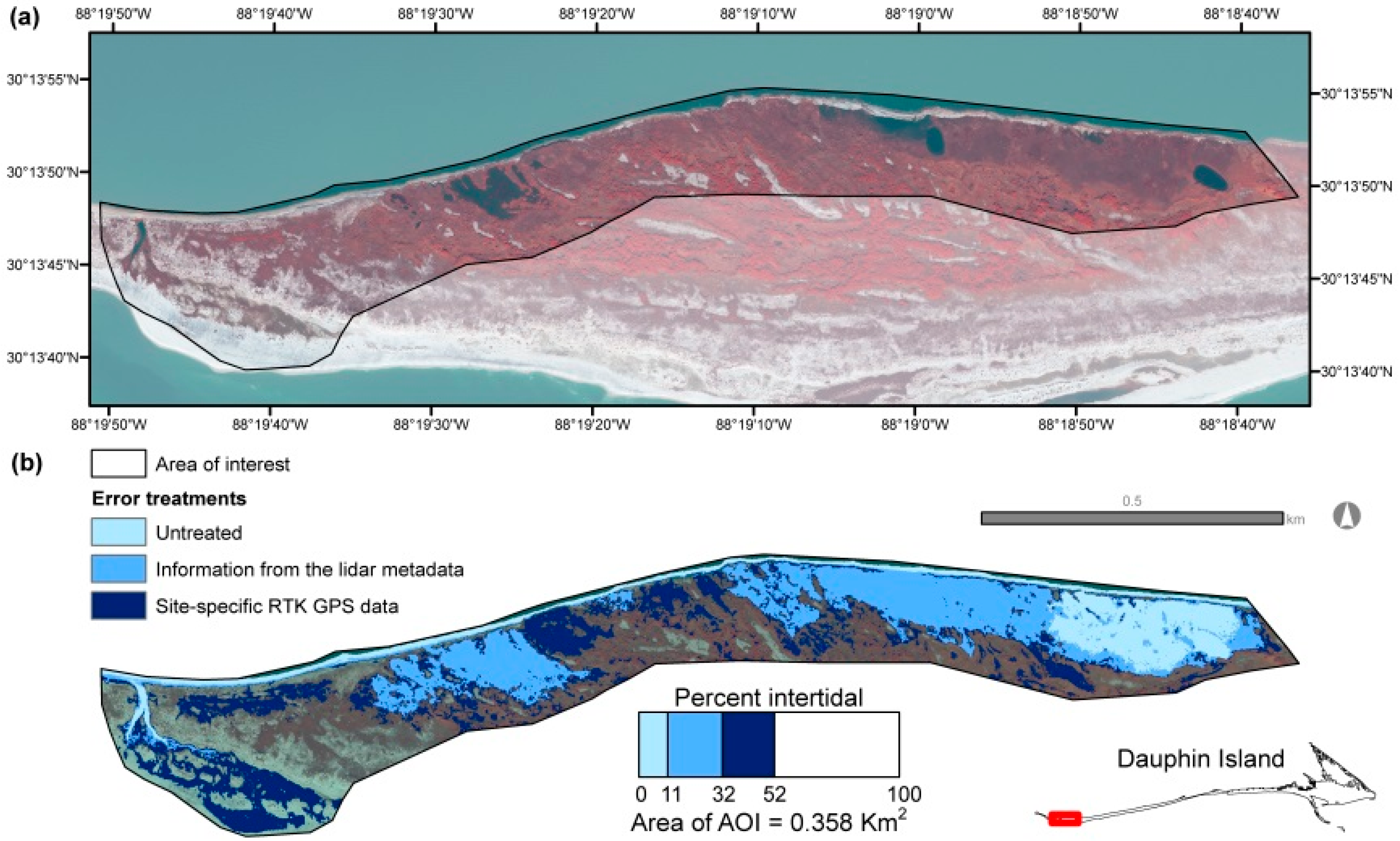
Figure 6, Figure 7 and Figure 8 show the extent of the intertidal area delineated for each error treatment for three different AOIs. Figure 6 includes back-barrier wetlands on the western tip of Dauphin Island. The percent of the AOI that contained intertidal areas increased by 190% when these areas were delineated using the DEM with error treatment using information from the lidar metadata. This figure increased to about 373% when intertidal areas were delineated using the DEM with error treatment using site-specific data. Figure 7 highlights an area with back-barrier wetlands near the island breach that occurred during Hurricane Katrina (named “Katrina Cut”). The percentage of the AOI that contained intertidal areas increased by 150% when these areas were delineated using the DEM with error treatment using information from the lidar metadata. This figure increased to about 294% when intertidal areas were delineated using the DEM with error treatment using site-specific RTK GPS data. Figure 8 includes intertidal marsh near Graveline Bay. Here, the differences amongst the three error treatments were much less pronounced; the difference between percent of the AOI that contained intertidal wetlands was ±10% for all three treatments.
3.3. Sensitivity Analysis
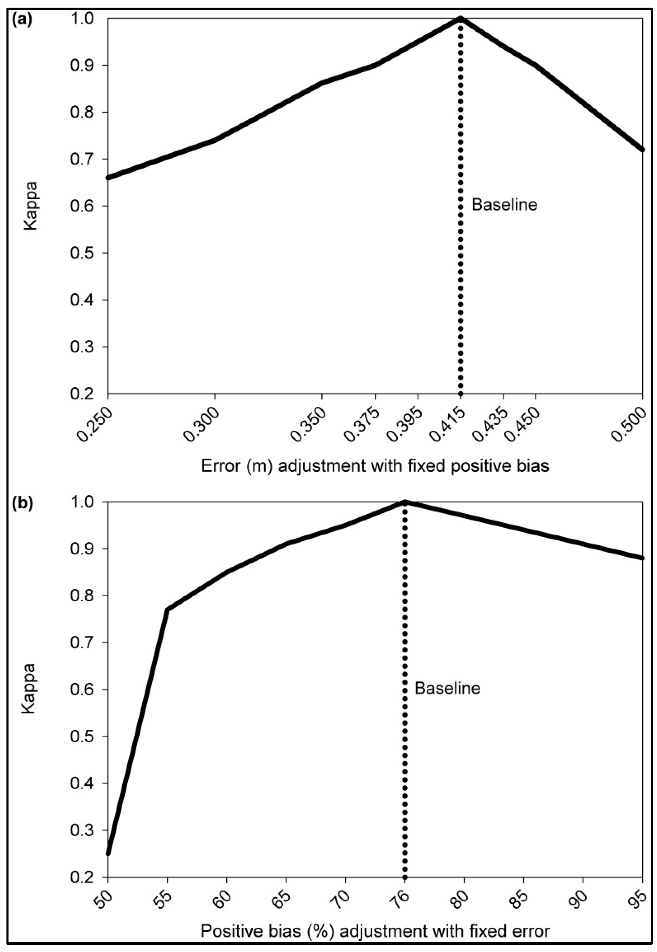
Figure 9 shows the results from the sensitivity analysis. Overall, adjustments to the error (Figure 9a) had a greater effect on the agreement of results with the baseline than adjustments to positive bias (Figure 9b). Scenarios had a Kappa of 0.85 with error values that ranged from 0.375 m to 0.450 m (baseline error = 0.415 m), whereas scenarios had a Kappa of 0.85 for positive bias that ranged from 60% to 95% (baseline positive bias = 76%). Results produced using a 50% positive bias (DEM overestimates elevation only 50% of the time) were very different from the baseline (Kappa = 0.25).
4. Discussion
In this study, we applied a simple probabilistic approach to more accurately use lidar data in coastal settings for delineation of the landward intertidal boundary. Our results confirm findings of others, which suggest that lidar DEMs can have a substantial level of vertical uncertainty in intertidal areas [17,18,19], and this uncertainty should be accounted for if data are directly used in classification algorithms for habitat mapping or for use in sea-level rise modeling efforts [42,43]. Our findings highlighted that optimal results with regards to the maximum identification of actual intertidal areas (i.e., highest producer’s accuracy) are likely produced when site-specific RTK GPS data are used. Due to the overall importance and the dynamic nature of intertidal ecosystems, a natural resource manager may prefer an approach that better ensures all intertidal areas are captured even if the methodology used may include some level of reasonable overestimation rather than underestimation. In the absence of site-specific data, using information from the lidar metadata to parameterize error and bias should provide better results than maps produced with error left untreated. With a lower vertical error estimate, the Monte Carlo analyses with information from the lidar metadata provided relatively balanced results with regards to producer’s accuracy and user’s accuracy. This was likely due to the moderate error and lower bias compared to the site-specific error and bias. Ultimately, the decision on how a researcher balances omission error (producer’s accuracy) or commission error (user’s accuracy) should be based on their research questions and mapping objectives.
By using connectivity constraints, we extended the Monte Carlo analyses to map areas likely to be intertidal wetlands. The impact of error treatments was explored for the entire island and for three different AOIs (Figure 6, Figure 7 and Figure 8). While the untreated DEM was more suitable for the intertidal marsh application near Graveline Bay (Figure 8), the differences were more magnified for other back-barrier marshes (Figure 6 and Figure 7). The similarity of the treatments for the marsh near Graveline Bay is likely the result of a lower overall elevation of the marsh platform in that area, but differences in vegetation community can also be a factor that affects localized lidar error, for example [18] (pp. 617–620). Clearly, a map of intertidal areas developed from untreated DEM would result in a gross underestimation of intertidal wetlands similar to results from other researchers [18,44]. However, both maps with treatment of error could provide reasonable intertidal wetland estimates based on lidar data alone or as an initial step that could be refined via minor manual photointerpretation. In other words, these maps can serve as a stand-alone inventory of area falling within the intertidal zone similar to the work of Liu et al. [29] or be used to as a foundation to develop a detailed habitat map [31].
The decision regarding use of site-specific RTK GPS data or information from the lidar metadata should be driven by project budget and research questions. In some cases, the lidar metadata may not provide sufficient information to assess the 95th percentile error for vegetated areas and estimate the bias. Under these circumstances, error treatment may only be feasible using error and bias values identified from literature that include analyses of lidar datasets with similar acquisition characteristics (e.g., point spacing) and vegetation community. We conducted a sensitivity analysis to provide insights on how results produced with minor adjustments to either error or bias compare to the results produced with site-specific RTK GPS data. Our results suggest selection of an appropriate error value may be more critical than bias; however, it seems important to have a bias value that is higher than 50% for study areas with vegetated areas. If it is necessary to rely on literature for error and bias values, then a thorough visual inspection of the results may be warranted to ensure parameters are producing reasonable results for the particular study area.
Due to the local scale of our study, we were able to transform vertical datum of the DEM from an orthometric datum to a locally relevant tidal datum using a tide gauge on the island. However, studies that cover a larger spatial extent may need to use a vertical datum transformation software, such as NOAA VDATUM [45] to transform orthometric datums to locally relevant tidal datums. This step can lead to additional vertical uncertainty, and if quantified for the transformation model, this uncertainty can be combined with the source data uncertainty and incorporated into the Monte Carlo simulations [27].
A byproduct of delineating the upper intertidal boundary is information on the extent and areal coverage of supratidal habitat. On barrier islands, supratidal areas include habitats such as beach, dune, and barrier flat (meadow, nonvegetated barrier flat, and forest). Monitoring these supratidal areas is equally important to resource managers [4] because these areas provide important habitat for resident and migratory shorebirds [46], neotropical migrants [47], and sea turtles [48]. Besides providing habitat for wildlife, dunes deliver erosion control for shorelines [49]. Dune crest elevation plays a critical role in the level of this protective capacity, and thus, in determining coastal vulnerability [49,50,51]. A Monte Carlo process similar to the one used in this study can be applied to determine areas with elevation that is greater than a typical extreme water level associated with storms using site-specific RTK GPS data collected in dune environments [31].
The objective of this study was to develop a straightforward approach for treating vertical uncertainty in lidar-based DEMs. This study leveraged RTK GPS data collected with a cluster sampling design that was obtained to serve as validation data for a habitat classification mapping effort [31]. For this reason, we chose to use a simple method of introducing spatial autocorrelation into the Monte Carlo processing by using a low-pass filter rather than a more complex approach, such as the weighted spatial dependence approach [26]. A more systematic sampling of lidar error in intertidal areas similar to the approaches applied by Medeiros et al. [17] or Buffington et al. [18] would allow for a more complex treatment of spatial autocorrelation. As stated earlier, analyses in this effort were restricted to intertidal areas above MSL due to the use of topographic lidar. The methodology used in this study could be modified to more accurately delineate the full intertidal zone (i.e., boundary between subtidal and intertidal habitats and boundary between supratidal and intertidal habitats) if used with topobathymetric lidar. Lidar intensity data has been shown to enhance habitat classifications in coastal environments [11,52]. Future efforts could explore the application of spatially variable error and bias based on a simple vegetation presence–absence classification based on lidar intensity. Additionally, the use of intensity information would allow researchers to extend this work to examine the habitat-specific impacts of not treating lidar error when delineating the intertidal zone. One potential issue related to this enhancement could be that high-quality intensity information may not be available for all lidar acquisitions. Finally, technological advancements like next-generation lidar sensors and on-demand lidar via UAS should greatly enhance how dynamic habitats like barrier islands are monitored. As data availability increases, this approach could be calibrated with next-generation lidar sensors such as single photon and Geiger-mode lidar platforms which enable data collection with much higher nominal point spacing (e.g., greater than 20 points per m2) as compared to conventional linear lidar (i.e., lidar used in this study was about 6 points per m2) [22] or data collected via on-demand lidar via an UAS [23,24]. Another potential improvement of using these methods with UAS data would be the ability to collect elevation data and optical imagery concurrently.
5. Conclusions
In intertidal areas, the elevation estimated from conventional aerial linear lidar can be much higher than the actual elevation due to dense vegetation cover. The uncertainty of DEMs is often not addressed for habitat mapping efforts, yet the level of uncertainty becomes critical when studying these low-relief and intertidal environments where centimeters can greatly influence the exposure to physically demanding abiotic conditions. In this study, we applied tide gauge information, RTK GPS data, and information from a detailed relative accuracy report that followed the ASPRS standards to simulate the propagation of elevation uncertainty into a DEM using Monte Carlo simulations. The primary objective of this study was to apply a simple approach to enhance results of automated intertidal area mapping using lidar data. We analyzed three different elevation error treatments which included leaving error untreated and treatments that used Monte Carlo simulations to incorporate elevation vertical uncertainty using lidar metadata and site-specific RTK GPS data, respectively.
Our work shows that the untreated DEM underestimated coverage of low-lying areas and intertidal areas. We found that the DEMs with treatment of error had higher producer’s accuracy and user’s accuracy for identifying low-lying areas below the EHWS. For the entire island, the percent intertidal lands increased by up to 80% when using Monte Carlo analyses to treat vertical uncertainty. Results from the sensitivity analysis suggest that it could be reasonable to use error and positive bias values from literature for similar environments, conditions, and lidar acquisition characteristics in the event that collection of site-specific data is not feasible and information in the lidar metadata is insufficient. In this event, we found that bias values may be less sensitive than error, although it is critical to select a bias value greater than 50% if the study area has abundant vegetation cover.
Results from this study should interest researchers that use lidar data in coastal morphology and habitat mapping studies, but especially those studying elevation-dependent ecological patterns and processes in coastal areas. The methodology outlined in this study could be used to develop stand-alone products with the simple aim of providing land managers with an accurate areal coverage of intertidal and supratidal habitats or to serve as a foundation for identification of tidal regimes for detailed habitat mapping efforts. The approach outlined in this study should be applicable to future technological advancements, such as next-generation lidar sensors and on-demand lidar via unmanned aerial systems.
Supplementary Materials
Data developed for this study are available online at https://doi.org/10.5066/F7125RVT.
Acknowledgments
This effort supported one component of a larger collaborative effort between the U.S. Army Corps of Engineers, the State of Alabama, and the U.S. Geological Survey, funded by the National Fish and Wildlife Foundation Gulf Environmental Benefit Fund (project ID: 45719) to investigate viable, sustainable restoration options that protect and restore the natural resources of Dauphin Island, Alabama. We acknowledge the U.S. Geological Survey’s National Geospatial Technical Operations Center and Digital Aerial Solutions, LLC. for airborne lidar data collection and processing. Any use of trade, firm, or product names is for descriptive purposes only and does not imply endorsement by the U.S. Government. This manuscript is submitted for publication with the understanding that the U.S. Government is authorized to reproduce and distribute reprints for Governmental purposes.
Author Contributions
N.M.E. and L.W. conceived and designed the study; N.M.E., S.M.B., R.H.D., L.C.F., and M.J.O. collected the data; N.M.E. and L.W. analyzed the data; N.M.E. wrote the paper; all authors contributed critically to subsequent drafts and gave final approval for publication.
Conflicts of Interest
The authors declare no conflict of interest.
References
- Oertel, G.F. The barrier island system. Mar. Geol. 1985, 63, 1–18. [Google Scholar] [CrossRef]
- Stutz, M.L.; Pilkey, O.H. Open-ocean barrier islands: Global influence of climatic, oceanographic, and depositional settings. J. Coast. Res. 2011, 27, 207–222. [Google Scholar] [CrossRef]
- Carruthers, T.J.B.; Beckert, K.; Schupp, C.A.; Saxby, T.; Kumer, J.P.; Thomas, J.; Sturgis, B.; Dennison, W.C.; Williams, M.; Fischer, T.; et al. Improving management of a mid-Atlantic coastal barrier island through assessment of habitat condition. Estuar. Coast. Shelf Sci. 2013, 116, 74–86. [Google Scholar] [CrossRef]
- Lucas, K.L.; Carter, G.A. Decadal changes in habitat-type coverage on Horn Island, Mississippi, U.S.A. J. Coast. Res. 2010, 26, 1142–1148. [Google Scholar] [CrossRef]
- Kindinger, J.L.; Buster, N.A.; Flocks, J.G.; Bernier, J.C.; Kulp, M.A. Louisiana Barrier Island Comprehensive Monitoring (BICM) Program Summary Report: Data and Analyses 2006 through 2010; U.S. Geological Survey: Reston, VA, USA, 2013; p. 86.
- Barbier, E.B.; Hacker, S.D.; Kennedy, C.; Koch, E.W.; Stier, A.C.; Silliman, B.R. The value of estuarine and coastal ecosystem services. Ecol. Monogr. 2011, 81, 169–193. [Google Scholar] [CrossRef]
- Cowardin, L.M.; Carter, V.; Golet, F.C.; LaRoe, E.T. Classification of Wetlands and Deepwater Habitats of the United States; United States Department of Interior, Fish and Wildlife Service: Washington, DC, USA, 1979; p. 134.
- Costanza, R.; de Groot, R.; Sutton, P.; van der Ploeg, S.; Anderson, S.J.; Kubiszewski, I.; Farber, S.; Turner, R.K. Changes in the global value of ecosystem services. Glob. Environ. Chang. 2014, 26, 152–158. [Google Scholar] [CrossRef]
- Madden, M.; Jones, D.; Vilcheck, L. Photointerpretation key for the Everglades vegetation classification system. Photogramm. Eng. Remote Sens. 1999, 65, 171–177. [Google Scholar]
- Maxa, M.; Bolstad, P. Mapping northern wetlands with high resolution satellite images and lidar. Wetlands 2009, 29, 248–260. [Google Scholar] [CrossRef]
- Chust, G.; Galparsoro, I.; Borja, A.; Franco, J.; Uriate, A. Coastal and estuarine habitat mapping, using lidar height and intensity and multi-spectral imagery. Estuar. Coast. Shelf Sci. 2008, 78, 633–643. [Google Scholar] [CrossRef]
- McCarthy, M.J.; Halls, J.N. Habitat mapping and change assessment of coastal environments: An examination of worldview-2, quickbird, and ikonos satellite imagery and airborne lidar for mapping barrier island habitats. ISPRS Int. J. Geo-Inf. 2014, 3, 297–325. [Google Scholar] [CrossRef]
- Zinnert, J.C.; Shiflett, S.A.; Via, S.; Bissett, S.; Dows, B.; Manley, P.; Young, D.R. Spatial–temporal dynamics in barrier island upland vegetation: The overlooked coastal landscape. Ecosystems 2016, 19, 685–697. [Google Scholar] [CrossRef]
- Klemas, V. Remote sensing of emergent and submerged wetlands: An overview, international journal of remote sensing. Int. J. Remote Sens. 2013, 34, 6286–6320. [Google Scholar] [CrossRef]
- Hodgson, M.E.; Bresnahan, P. Accuracy of airborne lidar-derived elevation: Empirical assessment and error budget. Photogramm. Eng. Remote Sens. 2004, 70, 331–339. [Google Scholar] [CrossRef]
- Su, J.; Bork, E. Influence of vegetation, slope, and lidar sampling angle on DEM accuracy. Photogramm. Eng. Remote Sens. 2006, 72, 1265–1274. [Google Scholar] [CrossRef]
- Medeiros, S.; Hagen, S.; Weishampel, J.; Angelo, J. Adjusting lidar-derived digital terrain models in coastal marshes based on estimated aboveground biomass density. Remote Sens. 2015, 7, 3507–3525. [Google Scholar] [CrossRef]
- Buffington, K.J.; Dugger, B.D.; Thorne, K.M.; Takekawa, J.Y. Statistical correction of lidar-derived digital elevation models with multispectral airborne imagery in tidal marshes. Remote Sens. Environ. 2016, 186, 616–625. [Google Scholar] [CrossRef]
- Schmid, K.A.; Hadley, B.C.; Wijekoon, N. Vertical accuracy and use of topographic lidar data in coastal marshes. J. Coast. Res. 2011, 27, 116–132. [Google Scholar] [CrossRef]
- Young, D.R.; Brantley, S.T.; Zinnert, J.C.; Vick, J.K. Landscape position and habitat polygons in a dynamic coastal environment. Ecosphere 2011, 2, 1–15. [Google Scholar] [CrossRef]
- Anderson, C.P.; Carter, G.A.; Funderbunk, W.R. The use of aerial RGB imagery and lidar in comparing ecological habitats and geomorphic features on a natural versus man-made barrier island. Remote Sens. 2016, 8, 602. [Google Scholar] [CrossRef]
- Stoker, J.M.; Abdullah, Q.A.; Nayegandhi, A.; Winehouse, J. Evaluation of single photon and geiger mode lidar for the 3D Elevation Program. Remote Sens. 2016, 8, 767. [Google Scholar] [CrossRef]
- Jaakkola, A.; Hyyppä, J.; Kukko, A.; Yu, X.; Kaartinen, H.; Lehtomäki, M.; Lin, Y. A low-cost multi-sensoral mobile mapping system and its feasibility for tree measurements. ISPRS J. Photogramm. Remote Sens. 2010, 65, 514–522. [Google Scholar] [CrossRef]
- Lin, Y.; Hyyppä, J.; Jaakkola, A. Mini-uav-borne lidar for fine-scale mapping. IEEE Geosci. Remote Sens. Lett. 2011, 8, 426–430. [Google Scholar] [CrossRef]
- Hunter, G.J.; Goodchild, M.F. Dealing with error in spatial databases: A simple case study. Photogramm. Eng. Remote Sens. 1995, 61, 529–537. [Google Scholar]
- Wechsler, S.P.; Kroll, C.N. Quantifying DEM uncertainty and its effect on topographic parameters. Photogramm. Eng. Remote Sens. 2006, 72, 1081–1090. [Google Scholar] [CrossRef]
- Cooper, H.M.; Fletcher, C.H.; Chen, Q.; Barbee, M.M. Sea-level rise vulnerability mapping for adaptation decisions using lidar DEMs. Prog. Phys. Geogr. 2013, 37, 745–766. [Google Scholar] [CrossRef]
- Leon, J.X.; Heuvelink, G.B.M.; Phinn, S.R. Incorporating DEM uncertainty in coastal inundation mapping. PLoS ONE 2014, 9, e108727. [Google Scholar] [CrossRef] [PubMed]
- Liu, H.; Sherman, D.; Gu, S. Automated extraction of shorelines from airborne light detection and ranging data andaccuracy assessment based on Monte Carlo simulation. J. Coast. Res. 2007, 23, 1359–1369. [Google Scholar] [CrossRef]
- American Society for Photogrammetry and Remote Sensing. ASPRS positional accuracy standards for digital geospatial data, November 2014. Photogramm. Eng. Remote Sens. 2015, 81, A1–A26. [Google Scholar]
- Enwright, N.M.; Borchert, S.B.; Day, R.H.; Feher, L.C.; Osland, M.J.; Wang, L.; Wang, H. Barrier Island Habitat Map and Vegetation Survey—Dauphin Island, Alabama, 2015; U.S. Geological Survey: Reston, VA, USA, 2017; p. 17.
- Otvos, E.G.J.; Carter, G.A. Hurricane degradation—Barrier development cycles, northeastern Gulf of Mexico: Landform evolution and island chain history. J. Coast. Res. 2008, 24, 463–478. [Google Scholar] [CrossRef]
- Morton, R.A. Historical changes in the Mississippi-Alabama barrier-island chain and the roles of extreme storms, sea level, and human activities. J. Coast. Res. 2008, 24, 1587–1600. [Google Scholar] [CrossRef]
- Heidemann, H.K. Lidar base specification. In U.S. Geological Survey Techniques and Methods; Heidemann, H.K., Ed.; U.S. Geological Survey: Reston, VA, USA, 2014; p. 67. [Google Scholar]
- Sugarbaker, L.J.; Constance, E.W.; Heidemann, H.K.; Jason, A.L.; Lukas, V.; Saghy, D.L.; Stoker, J.M. The 3D Elevation Program Initiative—A Call for Action; U.S. Geological Survey: Reston, VA, USA, 2014; p. 35.
- Arundel, S.T.; Archuleta, C.M.; Philips, L.A.; Roche, B.L.; Constance, E.W. 1-meter digital elevation model specification. In U.S. Geological Survey Techniques and Methods, Book 11; U.S. Geological Survey: Reston, VA, USA, 2015; p. 25. [Google Scholar]
- Cooper, H.M.; Chen, Q. Incorporating uncertainty of future sea-level rise estimates into vulnerability assessment: A case study in Kahului, Maui. Clim. Chang. 2013, 121, 635–647. [Google Scholar] [CrossRef]
- Poulter, B.; Halpin, P.N. Raster modelling of coastal flooding from sea-level rise. Int. J. Geogr. Inf. Sci. 2008, 22, 167–182. [Google Scholar] [CrossRef]
- Enwright, N.M.; Griffith, K.T.; Osland, M.J. Barriers to and opportunities for landward migration of coastal wetlands with sea-level rise. Front. Ecol. Environ. 2016, 14, 307–316. [Google Scholar] [CrossRef]
- Congalton, R.G.; Green, K. Assessing the Accuracy of Remotely Sensed Data Principles and Practices; CRC Press: Boca Raton, FL, USA, 2009. [Google Scholar]
- Cohen, J. A coefficient of agreement for nominal scales. Educ. Psychol. Meas. 1960, 20, 37–46. [Google Scholar] [CrossRef]
- Schile, L.M.; Callaway, J.C.; Morris, J.T.; Stralberg, D.; Parker, V.T.; Kelly, M. Modeling tidal marsh distribution with sea-level rise: Evaluating the role of vegetation, sediment, and upland habitat in marsh resiliency. PLoS ONE 2014, 9, e88760. [Google Scholar] [CrossRef] [PubMed]
- Alizad, K.; Hagen, S.C.; Morris, J.T.; Medeiros, S.C.; Bilskie, M.V.; Weishampel, J.F. Coastal wetland response to sea-level rise in a fluvial estuarine system. Earth's Future 2016, 4, 483–497. [Google Scholar] [CrossRef]
- Kidwell, D.M.; Dietrich, J.C.; Hagen, S.C.; Medeiros, S.C. An earth’s future special collection: Impacts of the coastal dynamics of sea level rise on low-gradient coastal landscapes. Earth's Future 2017, 5, 2–9. [Google Scholar] [CrossRef]
- Parker, B.B. The difficulties in measuring a consistently defined shoreline—The problem of vertical referencing. J. Coast. Res. 2003, SI 38, 44–56. [Google Scholar]
- Galbraith, H.; DesRochers, D.W.; Brown, S.; Reed, J.M. Predicting vulnerabilities of North American shorebirds to climate change. PLoS ONE 2014, 9, e108899. [Google Scholar] [CrossRef] [PubMed]
- Lester, L.A.; Ramierez, M.G.; Kneidel, A.H.; Heckscher, C.M. Use of a Florida Gulf Coast barrier island by spring trans-gulf migrants and the projected effects of sea level rise on habitat availability. PLoS ONE 2016, 11, e0148975. [Google Scholar] [CrossRef] [PubMed]
- Katselidis, K.A.; Schofield, G.; Stamou, G.; Dimopoulos, P.; Pantis, J.D. Employing sea-level rise scenarios to strategically select sea turtle nesting habitat important for long-term management at a temperate breeding area. J. Exp. Mar. Biol. Ecol. 2014, 450, 47–54. [Google Scholar] [CrossRef]
- Plant, N.G.; Thieler, E.R.; Passeri, D.L. Coupling centennial-scale shoreline change to sea-level rise and coastal morphology in the Gulf of Mexico using a Bayesian network. Earth's Future 2016, 4, 143–158. [Google Scholar] [CrossRef]
- Sallenger, A.H. Storm impact scale for barrier islands. J. Coast. Res. 2000, 16, 890–895. [Google Scholar]
- Stockdon, H.F.; Doran, K.J.; Thompson, D.M.; Sopkin, K.L.; Plant, N.G.; Sallenger, A.H. National Assessment of Hurricane-Induced Coastal Erosion Hazards—Gulf of Mexico; U.S. Geological Survey: Reston, VA, USA, 2012; p. 51.
- Brennan, R.; Webster, T.L. Object-oriented land cover classification of lidar-derived surfaces. Can. J. Remote Sens. 2006, 32, 162–172. [Google Scholar] [CrossRef]
Figure 1.
General overview of the study analyses. (a) Comparison of area with low-lying lands (i.e., elevation greater than or equal to the extreme high water spring tide level) and intertidal area using estimates from the three elevation error treatments; (b) Sensitivity analysis to assess how alternative error and bias values influence the identification of low-lying lands.
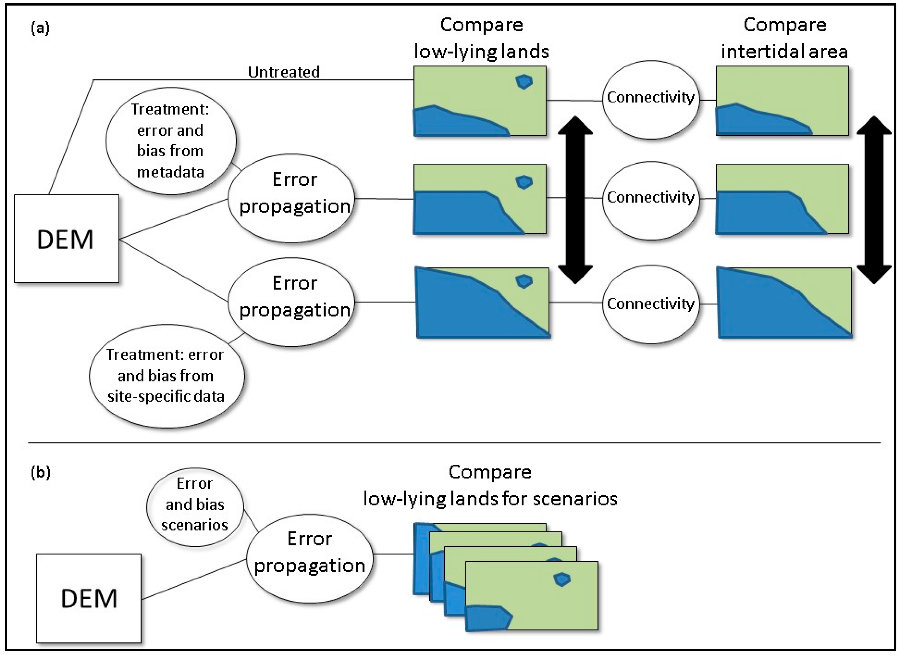
Figure 2.
Study area and the location of the tide gauge. Basemap source data is 0.3-m color-infrared orthoimagery acquired in 2015 by Digital Aerial Solutions, LLC (DAS; Riverview, FL, USA) and the U.S. Geological Survey (USGS).
Figure 2.
Study area and the location of the tide gauge. Basemap source data is 0.3-m color-infrared orthoimagery acquired in 2015 by Digital Aerial Solutions, LLC (DAS; Riverview, FL, USA) and the U.S. Geological Survey (USGS).
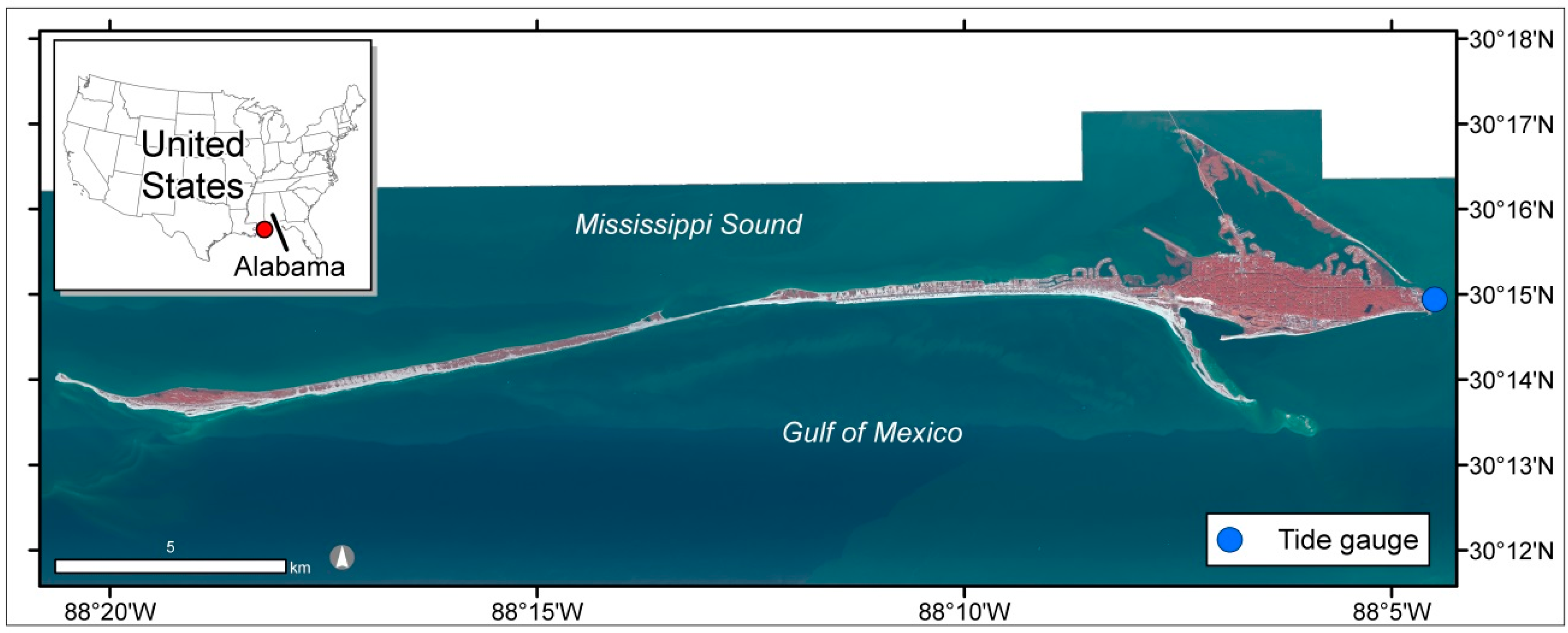
Figure 3.
Examples of habitat types where data were collected for the relative accuracy assessment of the 1-m digital elevation model (DEM). (a) Intertidal flat; (b) Intertidal marsh; (c) Meadow.
Figure 3.
Examples of habitat types where data were collected for the relative accuracy assessment of the 1-m digital elevation model (DEM). (a) Intertidal flat; (b) Intertidal marsh; (c) Meadow.
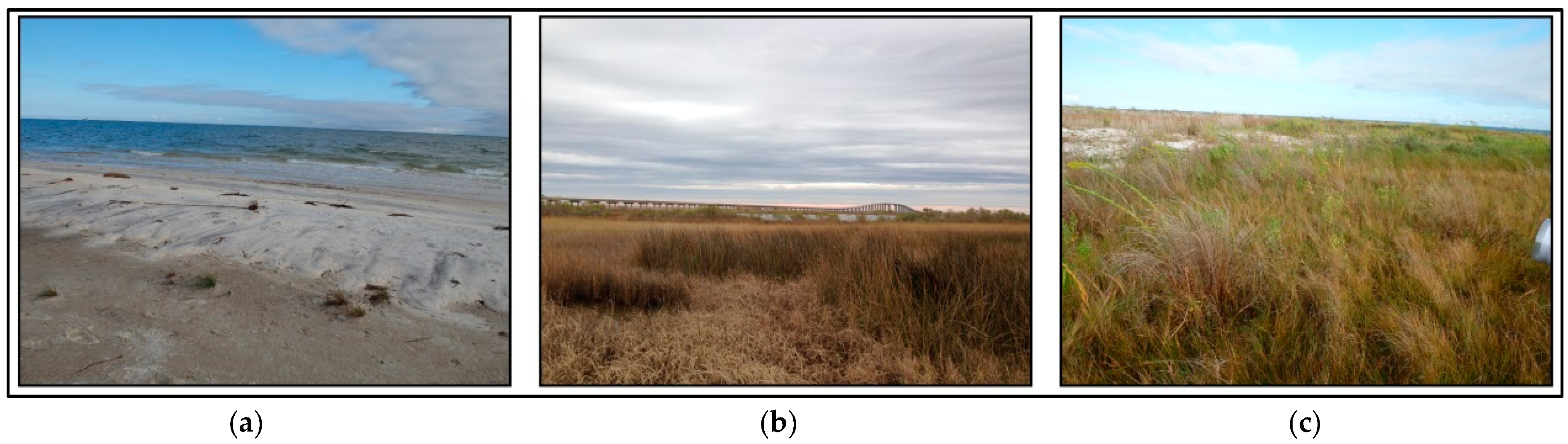
Figure 4.
An overview of the Monte Carlo error propagation process for estimating the probability of pixels being considered low-lying lands (i.e., elevation ≤ extreme high water spring), the presence–absence raster for pixels likely to be low-lying lands, and the presence–absence raster for pixels likely to be intertidal areas. DEM, digital elevation model; EHWS, extreme high water spring; PA, presence–absence raster.
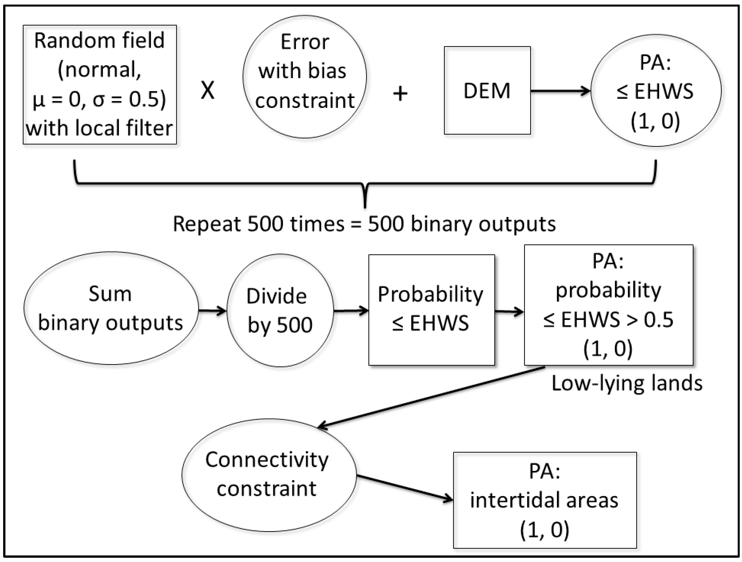
Figure 5.
Validation points for assessing the presence–absence rasters for low-lying lands (maps a–e). Basemap source data is 0.3-m color-infrared orthoimagery acquired in 2015 by the DAS and the USGS. (modified from [31] with permission)
Figure 5.
Validation points for assessing the presence–absence rasters for low-lying lands (maps a–e). Basemap source data is 0.3-m color-infrared orthoimagery acquired in 2015 by the DAS and the USGS. (modified from [31] with permission)

Figure 6.
Comparison of intertidal area delineated for each error treatment for back-barrier wetlands located near the western tip of Dauphin Island. (a) Color-infrared orthoimagery for the AOI. Imagery is 0.3-m color-infrared acquired in 2015 by DAS and the USGS; (b) Intertidal area delineated with each DEM within the AOI. To visualize the full extent of a given treatment it is necessary to consider areas with less sophisticated treatment(s) (e.g., include the extent of all treatments for visualizing the extent of the treatment with site-specific RTK GPS data). The percentage of total area within the AOI below delineated as intertidal (rounded to nearest percent) is shown graphically below the map. The location of the AOI is depicted on a generalized overview map of Dauphin Island [31]. AOI, area of interest; RTK GPS, Real-Time Kinematic Global Position System.

Figure 7.
Comparison of intertidal area delineated for each error treatment for back-barrier wetlands located east of Katrina Cut. (a) Color-infrared orthoimagery for the AOI. Imagery is 0.3-m color-infrared acquired in 2015 by DAS and the USGS; (b) Intertidal area delineated with each DEM within the AOI. To visualize the full extent of a given treatment it is necessary to consider areas with less sophisticated treatment(s) (e.g., include the extent of all treatments for visualizing the extent of the treatment with site-specific RTK GPS data). The percentage of total area within the AOI delineated as intertidal (rounded to nearest percent) is shown graphically below the map. The location of the AOI is depicted on a generalized overview map of Dauphin Island [31].
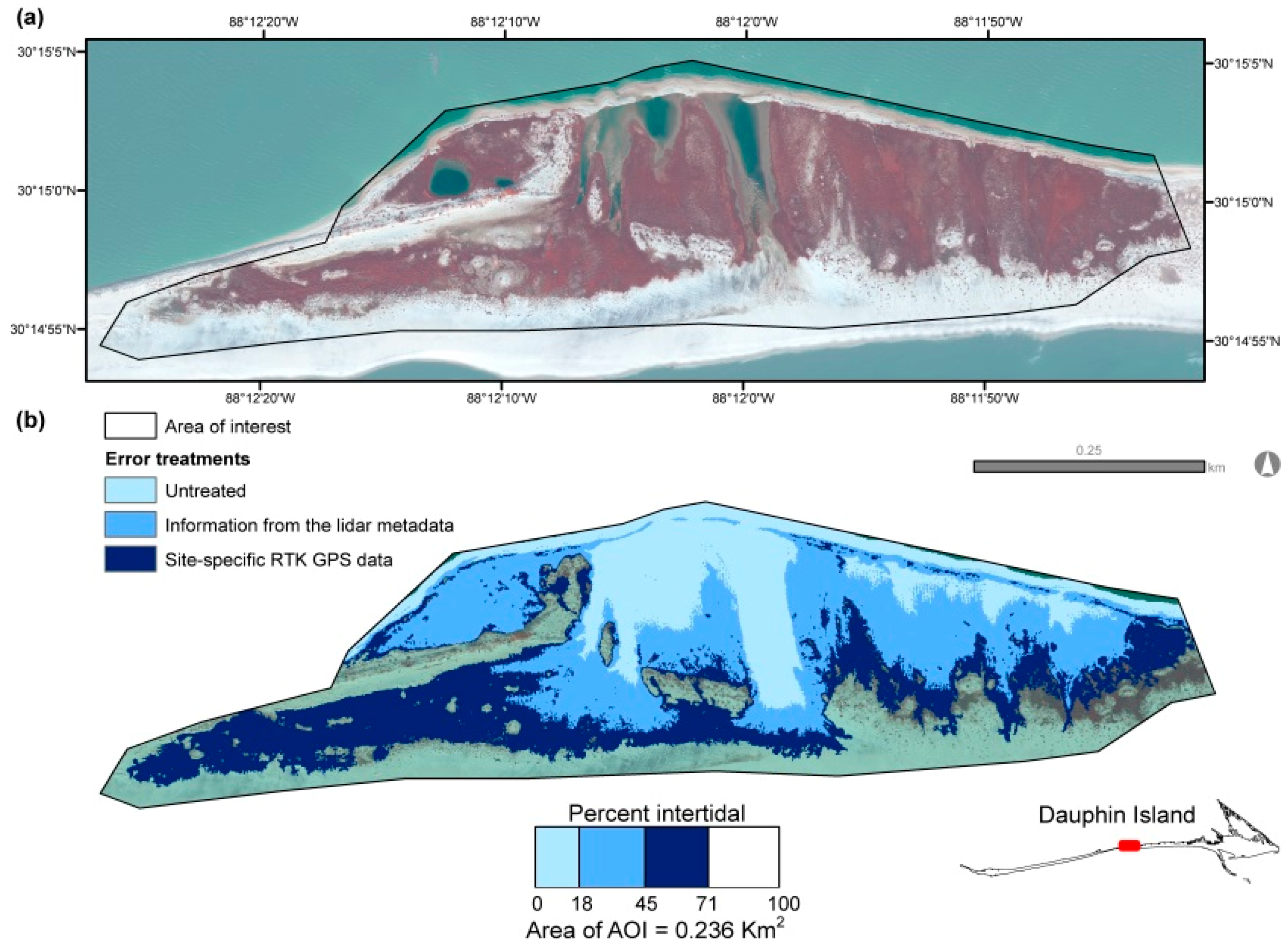
Figure 8.
Comparison of intertidal area delineated for each error treatment for back-barrier wetlands located near Graveline Bay. (a) Color-infrared orthoimagery for the AOI. Imagery is 0.3-m color-infrared acquired in 2015 by DAS and the USGS; (b) Intertidal area delineated with each DEM within the AOI. To visualize the full extent of a given treatment it is necessary to consider areas with less sophisticated treatment(s) (e.g., include the extent of all treatments for visualizing the extent of the treatment with site-specific RTK GPS data). The percentage of total area within the AOI delineated as intertidal (rounded to nearest percent) is shown graphically below the map. The location of the AOI is depicted on a generalized overview map of Dauphin Island [31].
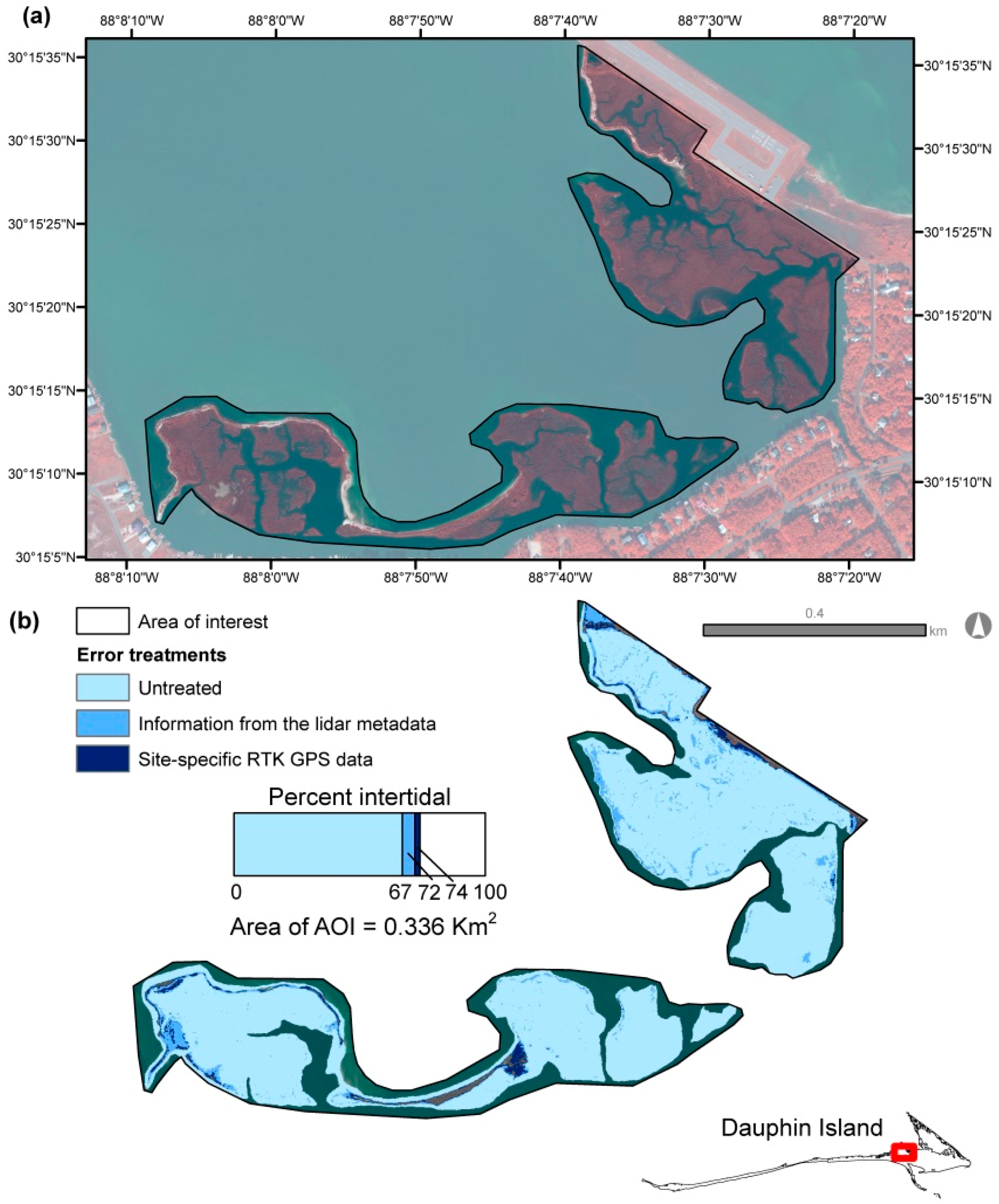
Figure 9.
Plots of the sensitivity analysis results. (a) Agreement between the baseline scenario and scenarios with alternative error values with a fixed positive bias (76%); (b) Agreement between the baseline scenario and scenarios with alternative positive bias values with a fixed error (0.415 m).


Table 1.
Relative error accuracy assessment between the 1-m DEM and the Real-Time Kinematic Global Position System (RTK GPS) observations.
Table 1.
Relative error accuracy assessment between the 1-m DEM and the Real-Time Kinematic Global Position System (RTK GPS) observations.
| Measure | Site-Specific RTK GPS Data | Lidar Metadata |
|---|---|---|
| Positive bias (%) | Nonvegetated (n = 7): 57.1 | Nonvegetated (n = 22): 36.3 |
| Vegetated (n = 55): 94.5 | Vegetated (n = 18): 72.2 | |
| Average (n = 62): 76.0 | Average (n = 40): 54.0 | |
| Skewness | 0.545 | 0.959 |
| 95th percentile error (m) | 0.415 | 0.326 |
Table 2.
Positive bias values used in the sensitivity analysis.
| Positive Bias (%) |
|---|
| 50 |
| 55 |
| 60 |
| 65 |
| 70 |
| 76 1 |
| 80 |
| 85 |
| 90 |
| 95 |
1 Baseline positive bias value.
Table 3.
Error values used in the sensitivity analysis.
| Error (m) |
|---|
| 0.250 |
| 0.300 |
| 0.350 |
| 0.375 |
| 0.395 |
| 0.415 1 |
| 0.435 |
| 0.450 |
| 0.500 |
1 Baseline error value.
Table 4.
Areal coverage, producer’s accuracy, and user’s accuracy for low-lying lands for each error treatment.
Table 4.
Areal coverage, producer’s accuracy, and user’s accuracy for low-lying lands for each error treatment.
| Error Treatment | Area of Low-Lying Lands (km2) | Producer’s Accuracy (%) | User’s Accuracy (%) |
|---|---|---|---|
| Untreated | 1.8 | 60.4 | 96.4 |
| Information from lidar metadata | 2.5 | 79.2 | 84.4 |
| Site-specific RTK GPS data | 3.1 | 87.5 | 68.9 |
Table 5.
Areal coverage of intertidal areas delineated for each error treatment.
| Error Treatment | Intertidal Area (km2) |
|---|---|
| Untreated | 1.6 |
| Information from lidar metadata | 2.3 |
| Site-specific RTK GPS data | 2.9 |
© 2017 by the authors. Licensee MDPI, Basel, Switzerland. This article is an open access article distributed under the terms and conditions of the Creative Commons Attribution (CC BY) license (http://creativecommons.org/licenses/by/4.0/).
Share and Cite
MDPI and ACS Style
Enwright, N.M.; Wang, L.; Borchert, S.M.; Day, R.H.; Feher, L.C.; Osland, M.J. The Impact of Lidar Elevation Uncertainty on Mapping Intertidal Habitats on Barrier Islands. Remote Sens. 2018, 10, 5. https://doi.org/10.3390/rs10010005
AMA Style
Enwright NM, Wang L, Borchert SM, Day RH, Feher LC, Osland MJ. The Impact of Lidar Elevation Uncertainty on Mapping Intertidal Habitats on Barrier Islands. Remote Sensing. 2018; 10(1):5. https://doi.org/10.3390/rs10010005
Chicago/Turabian StyleEnwright, Nicholas M., Lei Wang, Sinéad M. Borchert, Richard H. Day, Laura C. Feher, and Michael J. Osland. 2018. "The Impact of Lidar Elevation Uncertainty on Mapping Intertidal Habitats on Barrier Islands" Remote Sensing 10, no. 1: 5. https://doi.org/10.3390/rs10010005
Note that from the first issue of 2016, this journal uses article numbers instead of page numbers. See further details here.