Comparison of Pixel- and Object-Based Approaches in Phenology-Based Rubber Plantation Mapping in Fragmented Landscapes

Abstract

The increasing expansion of rubber plantations throughout East and Southeast Asia urgently requires improved methods for effective mapping and monitoring. The phenological information from rubber plantations was found effective in rubber mapping. Previous studies have mostly applied rule-pixel-based phenology approaches for rubber plantations mapping, which might result in broken patches in fragmented landscapes. This study introduces a new paradigm by combining phenology information with object-based classification to map fragmented patches of rubber plantations in Xishuangbanna. This research first delineated the time windows of the defoliation and foliation phases of rubber plantations by acquiring the temporal profile and phenological features of rubber plantations and natural forests through the Moderate Resolution Imaging Spectroradiometer (MODIS) Normalized Difference Vegetation Index (NDVI) data. To investigate the ability of finer resolution images at capturing the temporal profile or phenological information, 30 m resolution Landsat image data were used to capture the temporal profile, and a phenology algorithm to separate rubber plantations and natural forests was then defined. The derived phenology algorithm was used by both the object-based and pixel-based classification to investigate whether the object-based approach could improve the mapping accuracy. Whether adding the phenology information to the object-based classification could improve rubber plantation mapping accuracy in mountainous Xishuangbanna was also investigated. This resulted in three approaches: rule-pixel-based phenology, rule-object-based phenology, and nearest-neighbor-object-based phenology. The results showed that the rule-object-based phenology approaches (with overall accuracy 77.5% and Kappa Coefficients of 0.66) and nearest-neighbor-object-based phenology approach (91.0% and 0.86) achieved a higher accuracy than that of the rule-pixel-based phenology approach (72.7% and 0.59). The results proved that (1) object-based approaches could improve the accuracy of rubber plantation mapping compared to the pixel-based approach and (2) incorporating the phenological information from vegetation improved the overall accuracy of the thematic map.

1. Introduction

Monoculture rubber plantations (Hevea brasiliensis) have continuously expanded over tropical areas [1,2]. The global rubber plantation area has increased by 25% over the past two decades [3]. Driven by the global demands, the rubber plantation has rapidly expanded in Southeast Asia regions [4,5], with around 97% of global natural rubber supplied from Southeast Asia [4]. The expansion of rubber plantations is a primary driving factor of deforestation and of the decrease in swidden agricultural lands in Southeast Asia [6,7]. Even northern parts of the tropical belt, originally regarded as unsuitable for rubber plantations, have recently seen the large-scale growth of rubber plantations due to the use of cold-tolerant tree clones [8]. The expansion of rubber plantations has resulted in economic, social, and environmental consequences in new rubber-growing areas such as Xishuangbanna in China. The establishment of new plantations could benefit local economies and raise farmer incomes [9], but at the cost of disrupting traditional lifestyles, as well as damaging indigenous ecological knowledge, aesthetic, and cultural practices [8,10]. Ecologically, the expansion of rubber plantations has posed a series of environmental challenges such as reduced concentrations of soil organic carbon and increased carbon emissions, and has also resulted in reduced stream flows and water storage in the dry season [2,11,12]. As a result, regional environment and ecosystem services are severely affected.

The rapid growth of rubber plantations in the Xishuangbanna Region of Yunnan Province in China has displaced traditional agriculture and natural forests [4,13], and has therefore received much attention [2,14]. To better examine the ecological, social, and economic impacts of rubber plantations, improved spatial datasets of the distribution and changes in the extent of rubber plantations are needed. However, existing data on rubber plantation area dynamics and spatial patterns are not sufficient to support in-depth economic, social, and environmental studies [15]. Therefore, accurate mapping and monitoring of rubber plantations in Xishuangbanna are crucial to quantify and project the ecological and socio-economic impacts of rubber plantation expansion.

Enormous efforts have been devoted to mapping rubber plantations from remote sensing datasets, and these can generally be divided into two groups. One group of studies mapped rubber plantations using the image statistic approach on a single-date satellite image, usually at a medium or relatively fine spatial resolution such as Landsat, SPOT, and HJ [7,12,16,17,18]. Li et al. [12,16] successfully classified natural forests and rubber plantations using Landsat images. However, frequent cloud cover and limited data acquisition (16 day revisit interval by Landsat) in tropical regions often result in a limited availability of cloud-free Landsat images, thus constraining rubber plantation mapping in tropical regions. Additionally, the spectral characteristics of rubber plantations vary in different regions and different seasons, and plantations can exhibit similar spectral characteristics to the natural forest in a single image captured during the growing season [19,20]. Therefore, the other group of studies used time-series image analysis or a phenology-approach to map rubber plantations. For example, a Moderate Resolution Imaging Spectroradiometer (MODIS) sensor and China’s Feng-Yun-3A (FY-3A) have been used to map rubber plantations with temporal signals from images, and intra-annual temporal features or phenological characteristics [21,22]. Senf et al. (2013) [23] also examined phenological metrics of rubber plantations and other land cover types, and conducted classification based on the phenological signatures [21,22,23]. The results revealed that phenological characteristics can be successfully used to distinguish rubber plantations from natural forest. However, the coarse spatial resolution of MODIS limited its suitability for rubber plantation mapping in fragmented landscapes such as Xishuangbanna and Mountain Mainland Southeast Asia [4,19].

To overcome the limitations mentioned above, researchers combined cloud penetrating sensors with phenological information derived from optical satellite images to facilitate forest type classification [19,22]. For example, two studies combined the Advanced Land Observing Interferometric Synthetic Aperture Radar (ALOS-PALSAR) derived forest mask with phenological variables derived from Landsat to separate natural forests and rubber plantations [19,22]. The integration of Landsat and PALSAR overcame the cloud cover and mixed pixel problems of MODIS; however, although this method was effective in Hainan’s relatively smooth terrain [19,22], its application in Xishuangbanna’s fragmented and mountains landscape is challenged by the pixel classification. The current study focuses on two problems with current rubber plantation mapping approaches. First, relying on the RADAR (PALSAR) might result in a decreased accuracy as the complex and mountainous terrain in Xishuangbanna could cause amounts of noise in the resultant maps. Second, the pixel classification might result in too many small objects and broken patches.

Therefore, this study focused on the improvement of methods based on optical remote sensing data sets. It is therefore important to explore the applicability of fine resolution satellite images (e.g., Landsat, SPOT) to map rubber plantations in highly fragmented and heterogeneous landscapes. Second, it is assumed that an object-based approach could improve the classification accuracy of natural forests and rubber plantations in Xishuangbanna [19], as the object-related approach has been proven useful in the identification of large-scale artificial land uses [24,25,26] such as rubber plantations [17].

The objective of the current research is to improve the existing phenology-based rubber plantation mapping algorithm using object-based approaches. Specifically, two questions regarding mapping rubber plantations will be answered: (1) Is the phenology-based approach of mapping rubber plantation effective and robust in mountainous Xishuangbanna? (2) Can a combined object- and phenology-based approach improve the delineation of rubber plantations compared to a pixel- and phenology-based approach? In order to achieve this objective, this research integrated ground observational data and Landsat imagery to examine the phenological signatures of rubber plantations, and compared three different approaches (a rule-pixel-based phenology approach based on the pre-defined decision rule, a rule-object-based phenology approach based on the pre-defined decision rule, and a nearest-neighbor-object-based phenology approach by using Nearest Neighbor and object-based classification). It is expected to provide a general practical approach for regional rubber plantation mapping applicable in southern China and Southeast Asia in the near future.

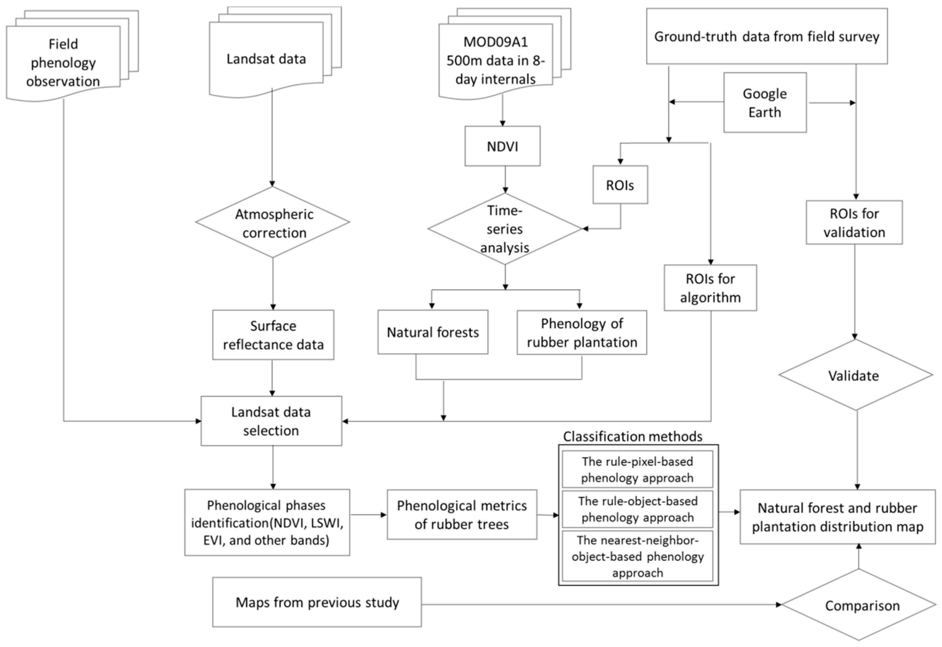
2. Materials and Methods

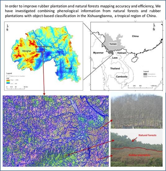
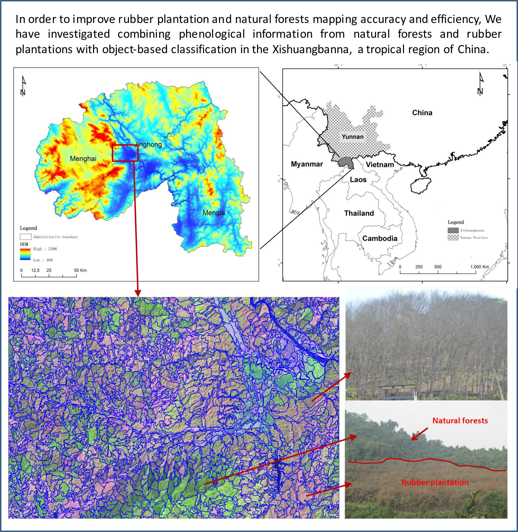
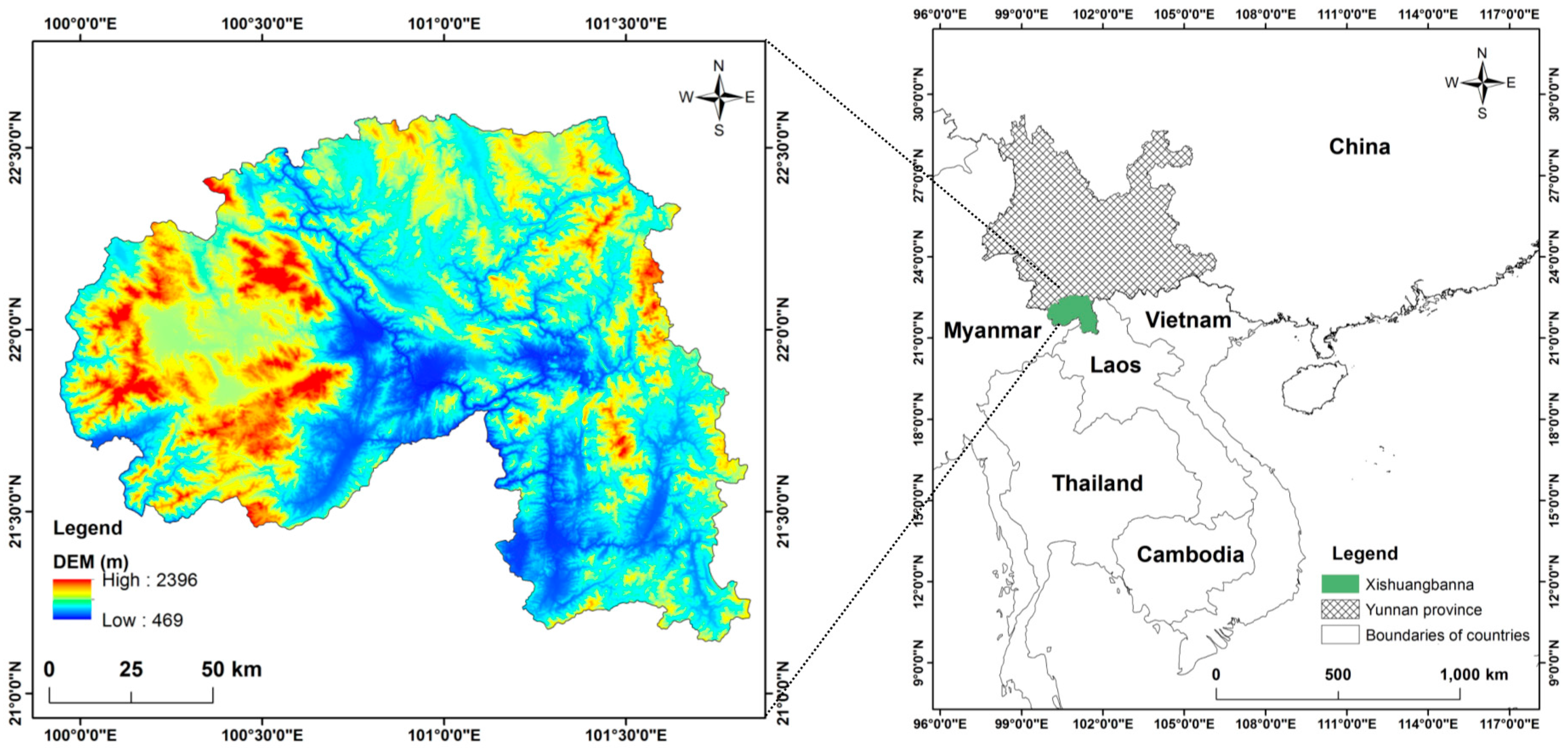
2.1. Study Area

Xishuangbanna Dai Autonomous Prefecture is situated between 21°08′ to 22°36′N latitudes and 99°56′ to 101°50′E longitudes in Yunnan Province, southwest China (Figure 1). It spans over an area of 19,150 km², and lies within the Indo-Burma global biodiversity hotspot area [27]. It borders Laos to the south and Myanmar to the southwest. The elevation varies from 475 m to 2430 m above sea level, and about 95% of the region is covered by mountains and hills. Xishuangbanna has a tropical moist climate, with a rainy season from May to October and a dry season from November to April, which includes a cool dry season from November to February and a hot dry season from March to April [28,29]. The dry season is characterized by relatively less rainfall, low temperatures, and fog. Heavy fog often occurs overnight in the cool dry season, while fog occurs in the morning only during the hot dry season [30]. The mean air temperature here is 21.7 °C, with the maximum of 25.7 °C in June and the minimum of 15.9 °C in January. There are four major forest types in Xishuangbanna: tropical rain forest, tropical seasonal moist forest, tropical monsoon forest, and tropical mountain evergreen broad-leaved forest [28]. Only the tropical monsoon forest is a deciduous forest, while the others are evergreen forests.

Rubber trees are native to the tropical rainforest of the Amazon Basin, and were not introduced into Xishuangbanna until the 1940s [31]. When rubber trees were first introduced, they were considered unsuitable for the northern marginal parts of the tropics such as Xishuangbanna, which featured cool winters and a distinct dry season [19]. Hybrid rubber varieties were then developed which could even be grown and harvested in cooler and drier climates [4]. In contrast to rubber trees in the Amazon, rubber trees in Xishuangbanna shed leaves in the coldest and driest months (January to March) and then undergo a rapid refoliation period [32].

2.2. Data Used and Preprocessing

2.2.1. Modis Data

In this study, the MODIS NDVI (Normalized Differential Vegetation Index) standard product coded as MOD09A1, with eight-day time intervals and at a 500 m spatial resolution, was obtained for the years 2001–2011. The 500 m MOD09A1 NDVI products were constructed to identify and examine the phenology of rubber trees and natural forests (Figure 2).

Temporal profiles of MODIS NDVI were extracted over eight sampling sites with rubber trees older than 25 years, as well as over another set of eight sampling sites for natural forests. The average NDVI value of rubber plantations decreased substantially from late October to early February of the following year, and the lowest NDVI values appeared in January and February, during the non-growing season. With the beginning of the growing season, NDVI increased rapidly from mid-February to October (Figure 2). Based on this intra-annual temporal analysis of NDVI, it was found that rubber plantations and natural forests can be clearly distinguished by MODIS during two periods: (1) early January to early February (defoliation period) and (2) February to early March (foliation period).

2.2.2. Landsat Data

To test the ability of Landsat images at capturing the temporal profile or phenological information, more images from January to April were required. The years of 2002–2003 were found to have more qualified data available than the other years. These eleven Landsat images pertaining to the defoliation and foliation season of rubber plantations from January to April were acquired from the USGS Earth Resources Observation and Science (EROS) Data Center (

Table 1. A list of Landsat TM/ETM+ images with the same orbit number (Path/Row 130/45) selected for this study.

Acquired Data	DOY	Sensor	Acquired Year
January 7	7	Landsat 5 TM	2002
January 26	26	Landsat 5 TM	2003
February 8	39	Landsat 5 TM	2002
February 11	42	Landsat 5 TM	2003
February 19	50	Landsat 7 ETM+	2003
February 28	59	Landsat 5 TM	2003
March 4	63	Landsat 7 ETM+	2002
March 28	87	Landsat 5 TM	2002
April 8	98	Landsat 7 ETM+	2002
April 21	111	Landsat 7 ETM+	2002
April 29	119	Landsat 5 TM	2002

) [33,34]. These images were L1T (level-one terrain-corrected) surface reflectance products [35,36] obtained during 2002–2003, with spatial resolutions of 30 m for reflective bands and 120 m for thermal bands (Table S1 [33]).

Temporal profiles of the three vegetation indices (VIs), which include two canopy greenness vegetation indices NDVI and EVI (Enhanced Vegetation Index)) and one moisture-related vegetation index: LSWI (Land Surface Water Index) [37] , were used to distinguish rubber plantations and natural forests by analyzing phenological differences. The NDVI [38] indicates canopy greenness or the amount of vegetation, the EVI shows higher resistance in atmospheric aerosol variations and soil background than NDVI [39], and the LSWI is more sensitive to the moisture of land surface and leaf water content [40]. The indices were calculated from Landsat data using the following formulas:

$$\mathrm{NDVI}=\frac{{\rho }_{nir}-{\rho }_{red}}{{\rho }_{nir}+{\rho }_{red}}$$

(1)

$$\mathrm{EVI}=2.5\times \frac{{\rho }_{nir}-{\rho }_{red}}{{\rho }_{nir}+6\times {\rho }_{red}-7.5\times {\rho }_{blue}+1}$$

(2)

$$\mathrm{LSWI}=\frac{{\rho }_{nir}-{\rho }_{swir1}}{{\rho }_{nir}+{\rho }_{swir1}}$$

(3)

where ${\rho }_{blue}$, ${\rho }_{red}$, ${\rho }_{nir}$, and ${\rho }_{swir1}$ are the reflectance values of Band 1 (Blue, 450–520 nm), Band 3 (Red, 630–690 nm), Band 4 (NIR, 760–900 nm), and Band 5 (Shortwave-infrared, SWIR1 for short hereafter, 1550–1750 nm) in Landsat TM/ETM+ sensors, respectively. Regarding EVI, the canopy background adjustment factor is 1, and the aerosol resistance weights are 6 and 7.5.

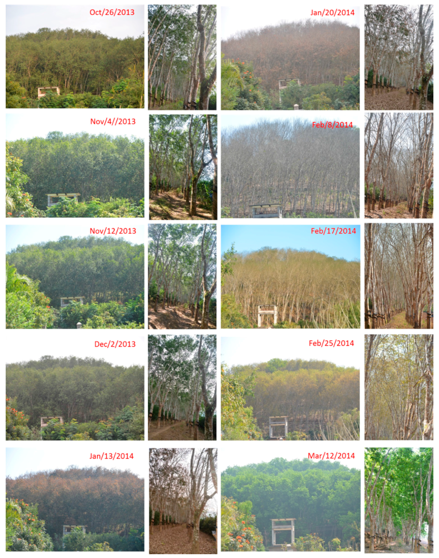
2.2.3. Training and Validation Data Collection and Field Observations of Rubber Plantation Phenology

The validation data of rubber plantations and natural forests were collected using a Global Position System receiver (Garmin eTrex) with a stratified random sampling approach in the field. Field surveys were conducted in 2011 and 2012. All these GPS point data (.shp) were converted to .kml files, which were then used as points of interest (POI). All these POIs were then digitized to regions of interest (ROIs) in Google Earth (GE) for training and thematic layer validation (Figure 3). The ROIs were extrapolated from POIs by linking the same period of high spatial resolution images in Google Earth which had a high geometric accuracy [41] (using historical imagery bar), and then the POI located homogeneous patch were digitized to ROI. Previous research has found this approach to be effective, capable of generating greater amounts of training and validation data than the point-based data [19].

The ground truth data were classified into three groups: (a) the first group of ROIs (11 natural forests and 11 rubber plantations) was used for the phenology phase (2001–2011) extraction through MODIS NDVI; (b) the second group of training ROIs of rubber plantation (11 ROIs of rubber, 37,559 pixels) and natural forest (11 ROIs of natural forests, 123,025 pixels) was used to conduct phenology feature analysis based on the Landsat images during the two foliation stages; and (c) the third group of points (30 rubber plantations from ground truth data with the trees ages older than ten years combined the other 114 points collected from the Google Earth) was used for accuracy assessments.

Field observations were conducted at a site in Xishuangbanna (101°16′1.43″E, 21°54′30.23″N) in order to observe the phenological developments of the rubber trees. The site was visited twice a month, and during every visit, photos were taken using a digital camera to record phenological conditions (including litterfall) (Figure 4).

2.3. Mapping Rubber Plantations Using Phenology at Regional Scale

Two of the eleven available Landsat images during the early foliation stage (19 February 2003) and late foliation stage (21 April 2002) were used for rubber plantation mapping. The phenological differences were apparent in the early and late foliation periods (Figure 5). The three derived vegetation indices (NDVI, EVI, and LSWI) and another six spectral bands (Blue, Green, Red, NIR, SWIR1, and SWIR2) were stacked for phenological feature extraction of rubber plantations. The selected images covered 87.3% of the total prefecture of Xishuangbanna (16,727 km² vs. 19,150 km² of the total prefecture).

2.3.1. Decision Rule

Based on the intra-annual temporal analysis of vegetation indices and bands, Landsat images for later classification should have distinct phenological features. Two Landsat 7 ETM+ images on 19 February 2003 and 21 April 2002 were then selected for signature analysis and later classification. The signature analysis was performed on the statistical analysis of the time series vegetation indices (NDVI, EVI, and LSWI) and bands (all non-thermal bands of Landsat images), which were extracted from ground truth sites of 11 ROIs (Region of Interest) comprising 37,559 pixels of rubber plantations and 11 ROIs comprising 123,025 pixels of natural forest (Figure 6).

At the early foliation stage, SWIR1, SWIR2, NDVI, LSWI, and EVI were identified with a higher ability to separate rubber plantations from natural forests than the other indices and spectral bands (Figure 6). At the early foliation stage, SWIR1 (0.263 ± 0.039) and SWIR2 (0.169 ± 0.026) of rubber plantations were higher than that of natural forests, with figures of 0.123 ± 0.030 and 0.052 ± 0.013, respectively (Figure 6a). Additionally, the NDVI (0.467 ± 0.023), LSWI (-0.086 ± 0.031), and EVI (0.276 ± 0.026) of rubber plantations at the same phenological stage were much lower than the natural forests, with figures of 0.783 ± 0.024, 0.362 ± 0.043, and 0.460 ± 0.087, respectively (Figure 6b).

During the late foliation stage, NIR, SWIR1, and EVI showed higher abilities to separate rubber plantations (0.357 ± 0.033, 0.189 ± 0.020, and 0.627 ± 0.053, respectively) from natural forests (0.279 ± 0.024, 0.131 ± 0.013, and 0.491 ± 0.039, respectively) than those of the other indices or spectral bands (Figure 6c,d). Hence, both the foliation stages showed a high potential to identify and separate rubber plantations from natural forests. In particular, SWIR1 and EVI performed better during these two foliation stages than the other indices or spectral bands (Figure 6). The decision rule was defined on the basis of a statistical analysis of SWIR1 and EVI, primarily the mean and standard deviation (SD). For example, the threshold of EVI for the rubber plantation in the defoliation stage ranged from 0.250 to 0.302 (mean ± SD), which was calculated by the mean EVI of the rubber plantation (0.276) and the standard deviation of EVI (0.026), and similarly, EVI values of natural forests ranged from 0.373 to 0.547 (Figure 6). After analyzing the data distribution, a mean value of 0.373 and 0.302 was used for rubber plantations in February. Rubber plantations and natural forests were found to be distinctive in SWIR1 and EVI values (Figure 6).

Through the signature analysis, the following decision rule was applied to identify the rubber plantation:

$$\mathrm{SWIR}1>=0.156\cup {\mathrm{EVI}}_{\left(\mathrm{Feb}\right)}<=0.338\cup {\mathrm{EVI}}_{\left(\mathrm{April}\right)}>=0.566$$

where ${\mathrm{EVI}}_{\left(\mathrm{Feb}\right)}$ and ${\mathrm{EVI}}_{\left(\mathrm{April}\right)}$ are the EVI value in February (19 February 2003) and April (21 April 2002), respectively.

The rubber plantation and natural forest distribution maps were classified using the stacked Landsat data with three approaches. Both the rule-pixel-based phenology approach and rule-object-based phenology approach used the above decision rule (Figure 7). The thematic maps for the classification included three classes: natural forests, rubber plantations, and other land use types.

2.3.2. Rule-Pixel-Based Phenology Approach

The rule-pixel-based phenology approach was conducted by combining Landsat and PALSAR imagery [19,42]. The 50 m PALSAR Orthorectified Mosaic data with the Fine Beam Dual (FBD) observational mode was downloaded from the ALOS Kyoto and Carbon Initiative (ftp://ftp.eorc.jaxa.jp/pub/ALOS/ftp/KC50). HH and HV polarization backscatters, the ratio, and the difference of HH and HV were considered in the process. PALSAR reflects land cover types with different backscatter characteristics, with a backscatter value higher for forests than non-forests (e.g., croplands and waterbodies) [19,42]. A map of forest and non-forest was generated from this PALSAR 50 m data with a decision tree classifier [19,42] (Figure 7). Generation of a forest map from the PALSAR data over a large area could be carried out without the limitation of seasons or regions. The generated 50 m forest map, which included rubber plantations and natural forests, was then used as a mask. The 50 m forest map was then resampled at a 30 m resolution to match the Landsat spatial resolution. The 30 m forest map was overlaid with the phenology information derived from time series Landsat imagery to generate a rubber plantation map (Figure 7). The phenology information from time series Landsat images can indicate whether a forest pixel is deciduous or evergreen through signature analysis derived from the threshold (or decision rule) (Figure 6). Additionally, rubber plantations were then extracted from the forest baseline map according to the decision rule derived from time series Landsat images (Figure 7).

2.3.3. Rule-Object-Based Phenology Approach

The rule-object-based phenology approach was carried out at two levels of object-based classification. The first step of object-based classification was segmentation, whereby the pixels of the image were first aggregated into the homogeneity units according to statistics and texture calculation, and were then subdivided into objects. This research used a multi-resolution segmentation approach, a bottom-up homogenous region aggregation technique based on certain criteria (e.g., scale, shape, and compactness criteria) [43]. The scale parameter determines the size of objects [43]. Due to the merging objects, the scale and shape of the objects are empirically determined by analysts [44,45,46]. Specifically, several experiments with different scales were tested and repeated for specific classification objects combined with their knowledge of objects feature and distribution, e.g., [13,43,44,46,47]. All non-thermal bands of the two Landsat images (six bands for each) were used for image segmentation, and this meant that a total of twelve bands were used. The parameters of image segmentation were set by a trial strategy (

Table 2. The multiresolution segmentation parameters.

Multi-Resolution Segmentation					Classification
Segment level	Scale	Shape	Compactness	Classes	Rule-object-based phenology approach	Nearest-neighbor-object-based phenology approach
Level 1	20	0.1	0.5	Vegetation/Non-vegetation	Nearest Neighbor classifier
				Nodata	Membership Function classifier
Level 2	10	0.1	0.5	Natural forests/Rubber Plantations	Decision tree classifier	Nearest Neighbor classifier
				Waterbodies/Other land use types Nodata	Membership Function classifier	Membership Function classifier

). Using the trial strategy, the parameters were set based on the equations of the parameters (Equations (1)–(5) in the supplementary document) and referencing other researchers (e.g., Liu et al. 2012 [18], Xu et al. 2014 [13]), and the segmented objects were then visually checked. The target objects (e.g., rubber plantation and natural forest) should have a clear boundary between objects, without being mixed with other classes. The classes were derived using the hierarchy approach on eCognition (Version 8.0, Trimble), and all the objects at each level were linked by a hierarchy approach.

The first level classes (i.e., vegetation, non-vegetation, and other land use types) were classified at the highest image object level with a coarse scale (20 in Table 2). More detailed classes were further defined at the second object level with a finer scale (10 in Table 2). The second level with its parent level vegetation was classified into natural forests, rubber plantations, and other land use types. For both object-based approaches, the first level used the same classifier of the Nearest Neighbor algorithm to classify the image objects into vegetation and non-vegetation. Additionally, the membership function was used to classify the Nodata from Vegetation/Non-vegetation. The membership function is an algorithm in eCognition using the fuzzy logic that determines the degree of membership of image objects to a class and also defines the relationship between feature values (Table 2) [43]. At the second level, both object-based approaches used the membership function classifier to classify waterbodies and other land use types, and the objects were assigned to waterbodies by spectral character analysis with waterbodies samples, and after that, all the other objects in the non-vegetation class were assigned as other land uses.

Both the rule-object-based and rule-pixel-based phenology approach applied a decision rule for classifying rubber plantations and natural forests. The decision rule for separating natural forests and rubber plantations was calculated from the signature analysis of candidate vegetation indices (NDVI, EVI, LSWI, and SWIR1) (Figure 6). The nearest-neighbor-object-based phenology approach used the Nearest Neighbor classifier to separate natural forests and rubber plantations, as detailed below.

2.3.4. Nearest-Neighbor-Object-Based Phenology Approach

For the nearest-neighbor-object-based phenology approach, a Nearest Neighbor classifier based on Feature Space Optimization was used for the separation rules between natural forests and rubber plantations. Moreover, all non-thermal bands of Landsat images (six bands) from early and late foliation stages were used for the image segmentation of the nearest-neighbor-object-based phenology approach. The nearest-neighbor-object-based phenology approach adopted the same segmentation approaches (the same scale, shape, and compactness in each level) and hierarchy classes as those of the rule-object-based phenology approach above (Table 2). Additionally, more vegetation indices of both early and late foliation stages were developed and fed into the Nearest Neighbor classifier. Several additional indices based on three VIs (NDVI, EVI, and LSWI) and SWIR1 were developed for the nearest-neighbor-object-based phenology approach with images from early foliation (Feb.) and late foliation stages (April), e.g., NDVI: NDVI_Feb − NDVI_April, NDVI_Feb + NDVI_April, NDVI_Feb/NDVI_April, NDVIratio = (NDVI_Feb − NDVI_April)/(NDVI_Feb + NDVI_April), and also similar calculations for EVI, LSWI, and SWIR1.

The Nearest Neighbor classifier of eCognition was applied to classify rubber plantations and natural forests. Fifty representative samples for each class were manually selected from the image objects. Then, the Nearest Neighbor classification algorithm was trained to differentiate each class by calculating the best combination of features (the three vegetation indices, SWIR1, and other developed indices). After this process, each image object was assigned to a corresponding class based on the maximum membership value calculated in the previous step.

The primary difference between the two object-based approaches was that the nearest-neighbor-object-based phenology approach used a sample-based Nearest Neighbor classifier (Table 2), while the rule-object-based phenology approach used a pre-defined decision rule classifier to classify natural forests and rubber plantations. Both the rule-object-based and nearest-neighbor-object-based phenology approaches used a membership function at the second level to classify waterbodies and other land use types (Table 2).

2.4. Validation and Comparison

The resultant thematic map of natural forests, rubber plantations, and other types of land cover at a 30 m spatial resolution was evaluated using a confusion matrix based on the points for validation. The points for validation were collected from previous ground truth data and from Google Earth imagery. For the accuracy assessment, there are 144 points including 30 ground truth points from rubber plantations older than ten years. The accuracy assessment data for natural forests were collected from Google Earth.

A total of 402 points were created from Google Earth to conduct accuracy assessments, including 144 points for natural forests, 114 points for rubber plantations (30 collected from the field), and 144 points for other types of land cover. A stratified random sampling approach using pre-existing land-cover maps (ALCM) has been adopted to generate the accuracy assessment points, which has been double-checked with Google Earth. All the resultant maps were assessed using these ROIs.

3. Results

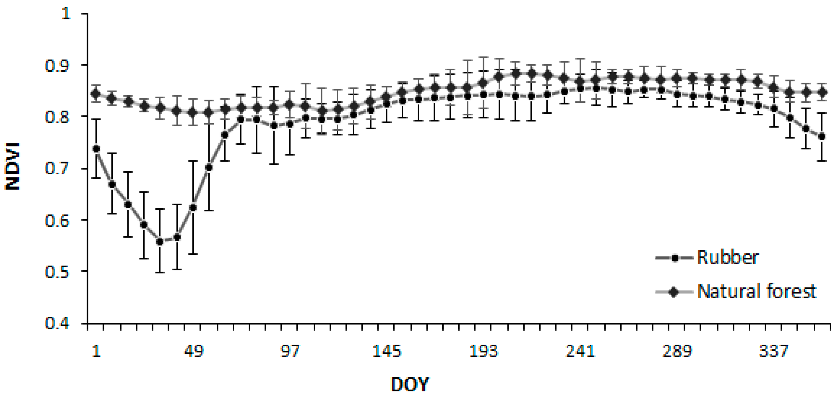
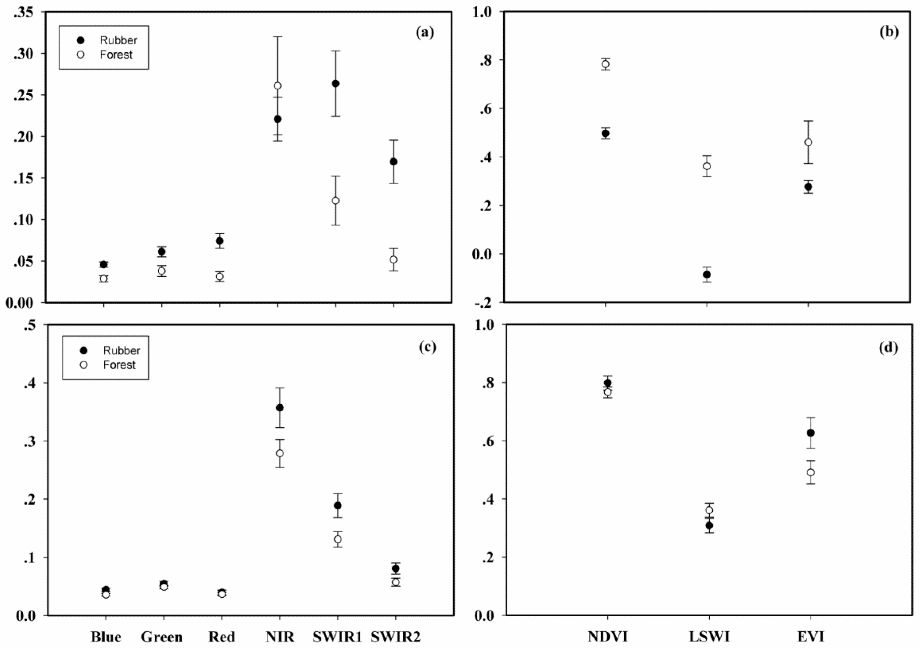
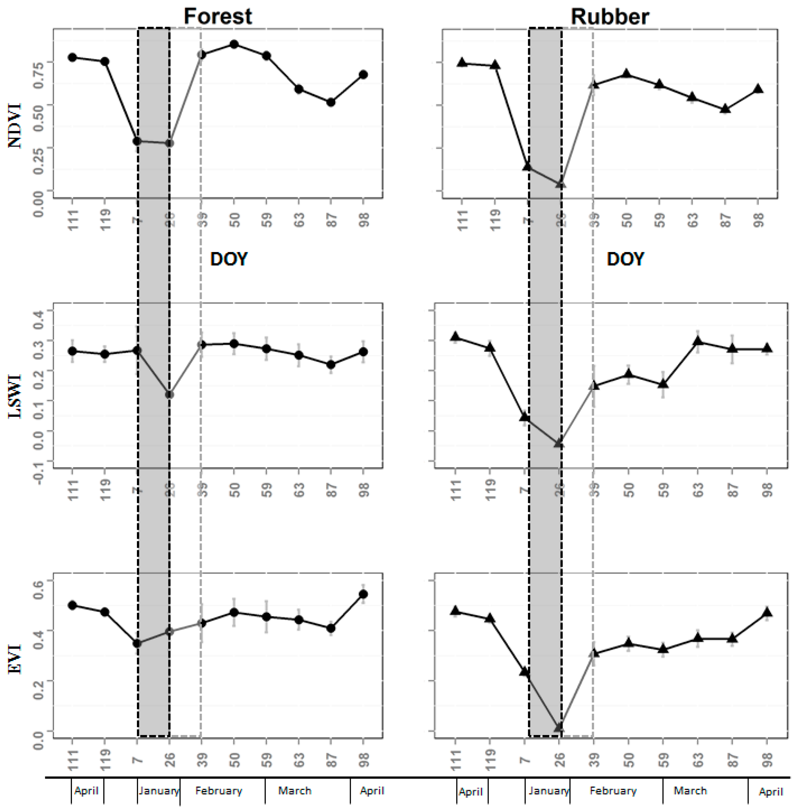
3.1. Rubber Plantation Phenology Characteristics in Xishuangbanna

The seasonal dynamics of MODIS NDVI of rubber plantations and natural forests showed that rubber plantations had a distinct phenology compared to natural forests only during the early and late (re)foliation periods (Figure 2). Hence, eleven Landsat TM/ETM+ images during 2002–2003 covering the corresponding defoliation/(re)foliation time were selected. Landsat images and results from field observations confirmed that during the dry season, rubber trees defoliated substantially in early January to early February. Thereafter, rubber trees underwent rapid (re)foliation and canopy recovery from February to early March (Figure 4 and Figure 8). However, during the rainy season (May to October), rubber plantations had similar NDVI levels to those of natural forests (Figure 2).

The Landsat derived vegetation indices showed that rubber plantations had lower NIR, NDVI, and EVI values than natural forests during the early foliation stage, and had higher NIR, NDVI, and EVI values than natural forests in the foliation stage (Figure 8), which suggests that rubber plantations can be separated from natural forests based on distinct phenological characteristics during these two stages.

A more detailed spectral analysis suggested that both foliation stages showed a high potential to identify and separate rubber plantations from natural forests. Additionally, the SWIR1 and EVI performed better in terms of identifying and separating rubber plantations from natural forests during these two foliation stages than the other indices or spectral bands (Figure 6). Therefore, the SWIR1 and EVI were used for decision rule extraction, which was defined as SWIR1 >= 0.156 and EVI (Feb) <= 0.338 and EVI (April) >= 0.566 for the rubber plantation. This decision rule to identify rubber plantations from natural forests was used for both the rule-pixel-based phenology and the rule-object-based phenology approach, but not for the nearest-neighbor-object-based phenology approach.

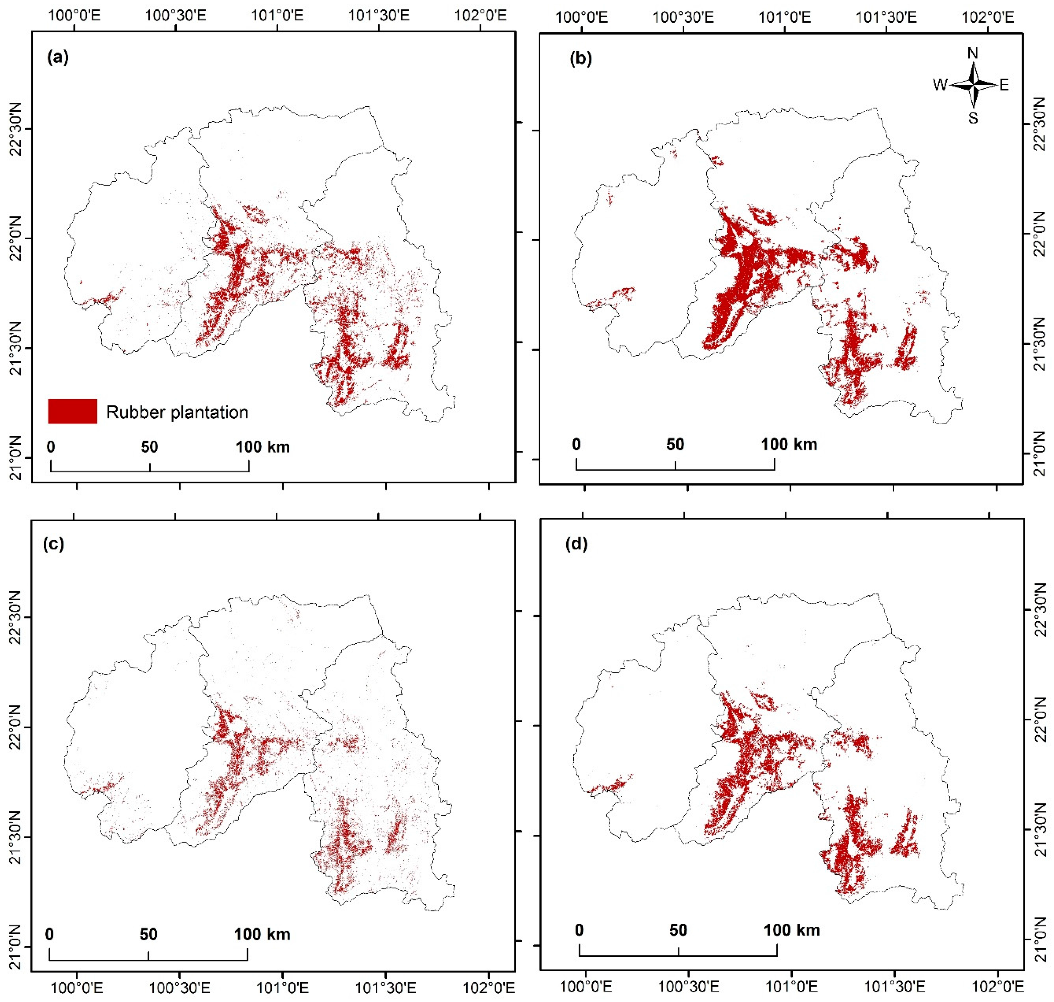
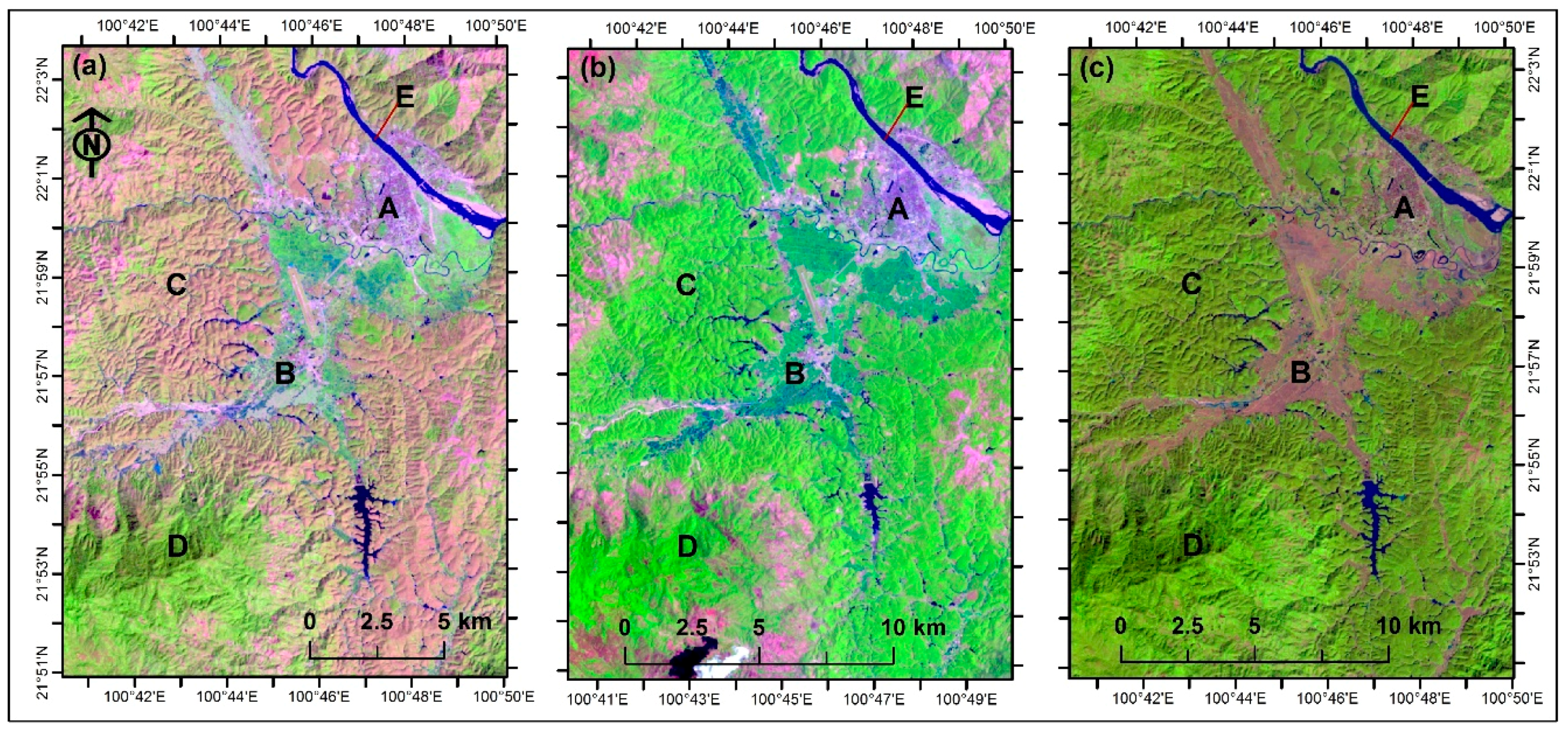
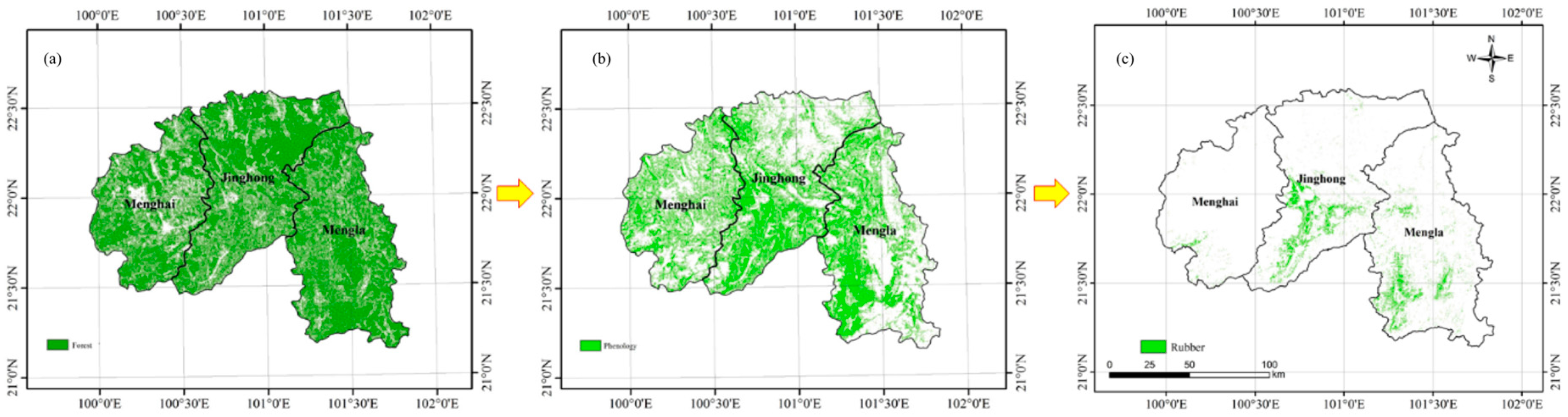
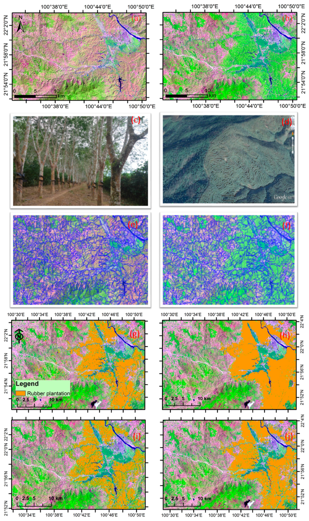
3.2. Rubber Plantation Map in Xishuangbanna and Accuracy Assessment

Two final rubber plantation maps were generated by the two object-based phenology approaches. The rubber plantation area in Xishuangbanna was estimated at 1342.7 km² according to the rule-object-based phenology approach, which was lower than the estimate of 1526.2 km² from previous research carried out by Xu et al. [13], while that of the nearest-neighbor-object-based phenology approach was 1866.0 km² (Figure 9).

The resulting natural forest and rubber plantation map by the nearest-neighbor-object-based phenology approach achieved a high accuracy according to the confusion matrix based on pixels derived from points collected by the ground truthing and Google Earth. The nearest-neighbor-object-based phenology approach achieved an overall accuracy of 91.0% and the Kappa coefficient was 0.86, which was higher than that of the rule-object-based phenology approach (77.5% and the Kappa coefficient was 0.66) (

Table 3. Accuracy assessment of the land cover classification map of Xishuangbanna based on Landsat 7 ETM+ images using the rule-pixel-based phenology approach, the rule-object-based phenology approach, and the nearest-neighbor-object-based phenology approach.

(A)
The Rule-Pixel-Based Phenology Approach	Class	Ground-Truth (Pixels)			Total Classified Pixels	User’s Accuracy
		Natural Forest	Rubber	Others
Classified results	Natural forest	130	80	16	226	57.5%
	Rubber	7	56	0	63	88.9%
	Others	7	8	128	143	89.5%
Total ground truth pixels		144	144	144	432
Producer’s accuracy		90.3%	38.9%	88.9%
Overall accuracy		72.7%
Kappa coefficient		0.59
(B)
The Rule-Object-Based Phenology Approach	Classes	Ground-Truth (Pixels)			Total Classified Pixels	User’s Accuracy
		Natural Forest	Rubber	Others
Classified results	Natural forest	137	53	6	196	69.9%
	Rubber	0	67	7	74	90.5%
	Others	7	24	134	162	80.9%
Total ground truth pixels		144	144	144	432
Producer’s accuracy		95.1%	46.5%	90.1%
Overall accuracy		77.5%
Kappa coefficient		0.66
(C)
The Nearest-Neighbor-Object-Based Approach	Classes	Ground-Truth (Pixels)			Total Classified Pixels	User’s Accuracy
		Natural Forest	Rubber	Others
Classified results	Natural forest	139	8	5	152	91.4%
	Rubber	5	130	15	150	86.7%
	Others	0	6	124	130	95.4%
Total ground truth pixels		144	144	144	432
Producer’s accuracy		96.5%	90.3%	86.1%
Overall accuracy		91.0%
Kappa coefficient		0.86

Notes: Others include arable lands, waterbodies, barren lands, build-up lands, and other land uses.

). The nearest-neighbor-object-based phenology approach discriminated better between natural forests and rubber plantations, and the producer’s accuracy (higher values indicate lower omission error) was higher than that of the rule-object-based phenology approach. The rule-object-based phenology approach using the pre-defined decision rule to differentiate natural forests and rubber plantation showed a lower producer’s accuracy (46.5%) of rubber plantations compared to that of the nearest-neighbor-object-based phenology approach (90.3%) (Table 3), but the user’s accuracy (higher values indicate lower commission error) of the rule-object-based phenology approach was higher than that of the nearest-neighbor-object-based phenology approach. The two object-based approaches achieved a higher accuracy than that observed by Senf, et al. [23] (63.6% with a pixel-based SWIR and EVI model). This disparity may be due to differences in resolution (250 m in the research of Senf, et al. [23] vs. 30 m in this research) (Table 3). The producer’s accuracy for rubber plantations identified via the rule-object-based phenology approach (46.5%) was higher than that of the rule-pixel-based phenology approach (38.9%) (Table 3). The interpretation accuracy of the rubber plantation using the nearest-neighbor-object-based phenology approach was larger than 85% for both the user’s and producer’s accuracy. The nearest-neighbor-object-based phenology approach showed the lowest omission error among the three approaches (Table 3).

4. Discussion

4.1. Performance of the Phenology-Based Approach for Rubber Plantation

The results of this study showed that phenological information of deciduous rubber plantations derived from Landsat images can be used to identify and map rubber plantations. The phenological information is quite useful for mapping rubber plantations in tropical China and has been applied to delineate rubber plantations from natural forests [19,23]. Most studies used only one image either from the defoliation or foliation phase to delineate rubber plantations from natural forests in Xishuangbanna [19,42,48,49]. For the proposed approach in this research, two images with distinct phenological information are required to effectively map rubber plantations and natural forests.

The current study demonstrated the utilities of phenological information for deciduous rubber plantation mapping in fragmented and mountainous rubber developing tropical regions. In the tropical regions, cloud cover can be an obstacle in acquiring optical satellite images [7,20], especially during the rainy season. Actually, both defoliation and foliation phases appeared in the dry season with relatively less cloud cover, which indicated that to map rubber plantation, it is still possible to get qualified relatively fine resolution optical images. The rule-object-based phenology and the nearest-neighbor-object-based phenology approach proposed in this study provide a solution to map finer resolution rubber plantations using finer resolution optical images than the MODIS. The phenological analysis based on Landsat images generated a finer extent and spatial configuration of rubber plantations than that of MODIS at 250 m or 500 m resolutions. In this research, the NDVI, LSWI, and EVI showed an evident decrease during the early foliation stage of rubber plantations. LSWI, in particular, can reach values below 0, while those of natural forests always remain above 0. This finding is consistent with Xiao, et al. [37], who found that LSWI values of natural evergreen forests were always higher than 0 over the whole year, while deciduous forest showed a period when LSWI fell below 0.

The phenology-based approach led to a comparatively higher accuracy than non-phenology-based approaches [7,12,20], and is more appropriate for a highly fragmented hilly rubber developing region [23,50].

4.2. Comparison of Object- vs. Pixel-Based Approaches in Phenology-Based Mapping

The object-based phenology approaches achieved a higher accuracy of rubber plantation mapping than rule-pixel-based phenology approaches (Table 3) in both the current study and other studies of Senf, et al. [23] and Dong, et al. [19]. The rule-object-based phenology approach was sufficient to extract rubber plantations and natural forests, but a higher accuracy was achieved using more spectral variables in the nearest-neighbor-object-based phenology approach, though this also resulted in a higher level of commission error. The higher accuracy of object-based results might be attributed to the identical image texture caused by land form and landscape terracing [7], which was demonstrated by high spatial resolution imageries in Google Earth and clear geographical distribution patterns [18] (Figure 10). The combination of phenological information and the pixel-based phenological approach also achieved a high accuracy; however, combining PALSAR and Landsat images seems to bring some uncertainties [19,42]. The pixel-based approach had a high omission in both natural forests and rubber plantations, which might be affected by topographic factors and stand age factors in the highly mountainous region of the study area [42]. The object-based approach can overcome this problem by its hierarchical classification, which is appropriate for complex classes (eCognition, Version 8.0, Trimble). The using of hierarchical classification makes better use of Landsat information rather than relying on other sensors to extract forest layers [19,48,49]. The separation of natural forests and rubber plantations by a decision rule in the rule-object-based phenology approach might be the reason for higher omission than that of the nearest-neighbor-object-based phenology approach, which used a Feature Space Optimization of the Nearest Neighbor classifier in eCognition.

4.4. Implication of Extensive Application

The time series MODIS and Landsat will be helpful in delineating the temporal seasonal dynamic patterns of rubber plantations. The phenology-based approaches have already been applied to other land uses (e.g., rice paddy land) with distinct phenological features. Another technique with great potential for plantation mapping is to identify bioclimatic factors related to defoliation and foliation (e.g., air temperature has been used by Dong, et al. [50] to identify phenology patterns of rice paddies). This has great potential to improve the efficiency and accuracy of plantation mapping and to apply in ecology researches in the Southeast Asia.

The object-based approaches in this research might also be able to improve the accuracy of paddy lands mapping over the rule-pixel-based phenology approach used by Dong, et al. [50]. The methods detailed in this research could furthermore be applied to other regions and plantations. The approaches used in this research could also be used with other optical satellite images (e.g., HJ (30 m)), or higher resolution satellite images (e.g., RapidEye (5 m), SPOT (5 m), GeoEye (0.5 m)) to facilitate the mapping of rubber plantations and other forest types.

4.5. Uncertainties of Rubber Plantation Mapping

A distinctive defoliation and a (re)foliation phase were identified by remote sensing in Xishuangbanna, which agrees with reports of other researchers based on site-based observations [32,51] and also the investigations in this study (Figure 4). However, with field data, the timing of the foliation was found to vary in different years and in each phenological event [52]. Additionally, there are phenological phase inconsistencies in different sites of the same region in one year. The inconsistency might relate to climate, latitude, elevation, rubber ages, and varieties [53], which could lead to the timing variations of rubber phenologies. Therefore, to get two images with distinct phenological information, it is advisable to check the phenological character of each candidate satellite image before further processing.

The defoliation and foliation phase was extracted by the deciduous features of rubber trees. However, the tropical monsoon forest also showed deciduous features in the dry season in Xishuangbanna [51]. Although the tropical monsoon forest was also found to shed leaves in the dry season, it showed a distinct pattern of leaf shedding (from January to mid-April) and leaf foliation (April to June) [51]. The distinct phenological pattern between rubber trees and tropical monsoon forests made it highly separate, especially from February to April.

5. Conclusions

This research combined phenological information for the mapping of natural forests and rubber plantations in Xishuangbanna. This approach combined phenological information derived from time series Landsat with object-based approaches. This combined method resulted in a 27% improvement of the Kappa coefficient compared to the rule-pixel-based phenology approach. This study revealed the advantages of the object-based strategy compared to the pixel-based strategy when using the phenological information to discriminate between rubber plantations and natural forests. Based on the above results, two conclusions were drawn. First, the phenology-based approach is effective and robust in rubber plantation mapping in mountainous Xishuangbanna, and Landsat is capable of capturing the phenological features of rubber plantations. According to the phenological features of rubber plantations, three distinct stages were identified: defoliation, foliation, and growth. Second, in highly fragmented regions, the object-based phenology approaches were able to better identify rubber plantations than the pixel-based phenology approach. Given the increasing availabilities of free satellite imagery, this object-based phenology approach could, in the future, be adopted in order to map rubber plantations annually at a finer resolution. However, the extensive application of this approach needs to consider phenological variation among rubber plantations in different regions. Moreover, the influence of site conditions (e.g., slope, aspect, and elevation), climate, rubber age, and varieties on the proposed approach also needs to be examined in order to further improve the accuracy of phenology-based regional mapping.

References

1. Koh, L.P.; Wilcove, D.S. Is oil palm agriculture really destroying tropical biodiversity? Conserv. Lett. 2008, 1, 60–64. [Google Scholar] [CrossRef]
2. Ziegler, A.D.; Fox, J.M.; Xu, J.C. The rubber juggernaut. Science 2009, 324, 1024–1025. [Google Scholar] [CrossRef] [PubMed]
3. Food and Agriculture Organization (FAO). Global Forest Resources Assessment 2010; FAO Forestry Paper; FAO: Rome, Italy, 2010. [Google Scholar]
4. Li, Z.; Fox, J.M. Mapping rubber tree growth in mainland southeast Asia using time-series MODIS 250 m NDVI and statistical data. Appl. Geogr. 2012, 32, 420–432. [Google Scholar] [CrossRef]
5. Prachaya, J. London and Bangkok; Rubber Economist Quarterly Report; The Rubber Economist Ltd.: Bangkok, Thailand, 2009. [Google Scholar]
6. Fox, J.; Vogler, J.B. Land-use and land-cover change in montane mainland Southeast Asia. Environ. Manag. 2005, 36, 394–403. [Google Scholar] [CrossRef] [PubMed]
7. Zhai, D.-L.; Cannon, C.H.; Slik, J.W.F.; Zhang, C.-P.; Dai, Z.-C. Rubber and pulp plantations represent a double threat to Hainan’s natural tropical forests. J. Environ. Manag. 2012, 96, 64–73. [Google Scholar] [CrossRef] [PubMed]
8. Xu, J.C.; Ma, E.T.; Tashi, D.; Fu, Y.S.; Lu, Z.; Melick, D. Integrating sacred knowledge for conservation: Cultures and landscapes in southwest China. Ecol. Soc. 2005, 10, 7. [Google Scholar] [CrossRef]
9. Sturgeon, J.C. Cross-border rubber cultivation between China and Laos: Regionalization by Akha and Tai rubber farmers. Singap. J. Trop. Geogr. 2013, 34, 70–85. [Google Scholar] [CrossRef]
10. Fu, Y.; Chen, J.; Guo, H.; Hu, H.; Chen, A.; Cui, J. Agrobiodiversity loss and livelihood vulnerability as a consequence of converting from subsistence farming systems to commercial plantation-dominated systems in Xishuangbanna, Yunnan, China: A household level analysis. Land Degrad. Dev. 2010, 21, 274–284. [Google Scholar] [CrossRef]
11. Guardiola-Claramonte, M.; Troch, P.A.; Ziegler, A.D.; Giambelluca, T.W.; Durcik, M.; Vogler, J.B.; Nullet, M.A. Hydrologic effects of the expansion of rubber (Hevea brasiliensis) in a tropical catchment. Ecohydrology 2010, 3, 306–314. [Google Scholar] [CrossRef]
12. Li, H.M.; Ma, Y.X.; Aide, T.M.; Liu, W.J. Past, present and future land-use in Xishuangbanna, China and the implications for carbon dynamics. For. Ecol. Manag. 2008, 255, 16–24. [Google Scholar] [CrossRef]
13. Xu, J.; Grumbine, R.E.; Beckshafer, P. Landscape transformation through the use of ecological and socioeconomic indicators in Xishuangbanna, Southwest China, Mekong region. Ecol. Indic. 2014, 36, 749–756. [Google Scholar] [CrossRef]
14. Qiu, J. Where the rubber meets the garden. Nature 2009, 457, 246–247. [Google Scholar] [CrossRef] [PubMed]
15. Grogan, K.; Pflugmacher, D.; Hostert, P.; Kennedy, R.; Fensholt, R. Cross-border forest disturbance and the role of natural rubber in mainland Southeast Asia using annual Landsat time series. Remote Sens. Environ. 2015, 169, 438–453. [Google Scholar] [CrossRef]
16. Li, H.M.; Aide, T.M.; Ma, Y.X.; Liu, W.J.; Cao, M. Demand for rubber is causing the loss of high diversity rain forest in SW China. Biodivers. Conserv. 2007, 16, 1731–1745. [Google Scholar] [CrossRef]
17. Liu, X.; Feng, Z.; Jiang, L. Application of decision tree classification to rubber plantations extraction with remote sensing. Trans. Chin. Soc. Agric. Eng. 2013, 29, 163–172. [Google Scholar]
18. Liu, X.; Feng, Z.; Jiang, L.; Zhang, J. Rubber plantations in Xishuangbanna: Remote sensing identification and digital mapping. Resour. Sci. 2012, 34, 1769–1780. [Google Scholar]
19. Dong, J.; Xiao, X.; Chen, B.; Torbick, N.; Jin, C.; Zhang, G.; Biradar, C. Mapping deciduous rubber plantations through integration of PALSAR and multi-temporal Landsat imagery. Remote Sens. Environ. 2013, 134, 392–402. [Google Scholar] [CrossRef]
20. Li, Z.; Fox, J.M. Integrating mahalanobis typicalities with a neural network for rubber distribution mapping. Remote Sens. Lett. 2011, 2, 157–166. [Google Scholar] [CrossRef]
21. Chen, H.; Chen, X.; Chen, Z.; Zhu, N.; Tao, Z. A primary study on rubber acreage estimation from modis-based information in Hainan. Chin. J. Trop. Crops 2010, 31, 1181–1185. [Google Scholar]
22. Dong, J.; Xiao, X.; Sheldon, S.; Biradar, C.; Duong, N.D.; Hazarika, M. A comparison of forest cover maps in mainland Southeast Asia from multiple sources: PALSAR, MERIS, MODIS and FRA. Remote Sens. Environ. 2012, 127, 60–73. [Google Scholar] [CrossRef]
23. Senf, C.; Pflugmacher, D.; van der Linden, S.; Hostert, P. Mapping rubber plantations and natural forests in Xishuangbanna (Southwest China) using multi-spectral phenological metrics from MODIS time series. Remote Sens. 2013, 5, 2795–2812. [Google Scholar] [CrossRef]
24. Cheng, G.; Han, J.; Guo, L.; Liu, Z.; Bu, S.; Ren, J. Effective and efficient midlevel visual elements-oriented land-use classification using VHR remote sensing images. IEEE Trans. Geosci. Remote Sens. 2015, 53, 4238–4249. [Google Scholar] [CrossRef]
25. Cheng, G.; Guo, L.; Zhao, T.; Han, J.; Li, H.; Fang, J. Automatic landslide detection from remote-sensing imagery using a scene classification method based on BoVW and pLSA. Int. J. Remote Sens. 2013, 34, 45–59. [Google Scholar] [CrossRef]
26. Cheng, G.; Han, J.; Zhou, P.; Guo, L. Multi-class geospatial object detection and geographic image classification based on collection of part detectors. ISPRS J. Photogramm. Remote Sens. 2014, 98, 119–132. [Google Scholar] [CrossRef]
27. Mittermeier, R.A.; Gil, P.R.; Hoffman, M.; Pilgrim, J.; Brooks, T.; Mittermeier, C.G.; Lamoreux, J.; da Fonseca, G.A.B. Hotspots Revisited: Earth’s Biologically Richest and Most Endangered Terrestrial Ecoregions; Conservation International: Hongkong, China, 2005. [Google Scholar]
28. Zhu, H.; Cao, M.; Hu, H.B. Geological history, flora, and vegetation of Xishuangbanna, Southern Yunnan, China. Biotropica 2006, 38, 310–317. [Google Scholar] [CrossRef]
29. Liu, W.J.; Liu, W.Y.; Li, P.J.; Gao, L.; Shen, Y.X.; Wang, P.Y.; Zhang, Y.P.; Li, H.M. Using stable isotopes to determine sources of fog drip in a tropical seasonal rain forest of Xishuangbanna, SW China. Agric. For. Meteorol. 2007, 143, 80–91. [Google Scholar] [CrossRef]
30. Song, Q.; Lin, H.; Zhang, Y.; Tan, Z.; Zhao, J.; Zhao, J.; Zhang, X.; Zhou, W.; Yu, L.; Yang, L.; et al. The effect of drought stress on self-organization in a seasonal tropical rainforest. Ecol. Model. 2013, 265, 136–139. [Google Scholar] [CrossRef]
31. Xu, J. The political, social, and ecological transformation of a landscape—The case of rubber in Xishuangbanna, China. Mt. Res. Dev. 2006, 26, 254–262. [Google Scholar]
32. Guardiola-Claramonte, M.; Troch, P.A.; Ziegler, A.D.; Giambelluca, T.W.; Vogler, J.B.; Nullet, M.A. Local hydrologic effects of introducing non-native vegetation in a tropical catchment. Ecohydrology 2008, 1, 13–22. [Google Scholar] [CrossRef]
33. Roy, D.P.; Wulder, M.A.; Loveland, T.R.; Allen, R.G.; Anderson, M.C.; Helder, D.; Irons, J.R.; Johnson, D.M.; Kennedy, R.; Scambos, T.A.; et al. Landsat-8: Science and product vision for terrestrial global change research. Remote Sens. Environ. 2014, 145, 154–172. [Google Scholar] [CrossRef]
34. Wulder, M.A.; White, J.C.; Goward, S.N.; Masek, J.G.; Irons, J.R.; Herold, M.; Cohen, W.B.; Loveland, T.R.; Woodcock, C.E. Landsat continuity: Issues and opportunities for land cover monitoring. Remote Sens. Environ. 2008, 112, 955–969. [Google Scholar] [CrossRef]
35. Masek, J.G.; Vermote, E.F.; Saleous, N.E.; Wolfe, R.; Hall, F.G.; Huemmrich, K.F.; Gao, F.; Kutler, J.; Lim, T.K. A Landsat surface reflectance dataset for North America, 1990–2000. IEEE Geosci. Remote Sens. Lett. 2006, 3, 68–72. [Google Scholar] [CrossRef]
36. Vermote, E.F.; El Saleous, N.; Justice, C.O.; Kaufman, Y.J.; Privette, J.L.; Remer, L.; Roger, J.C.; Tanré, D. Atmospheric correction of visible to middle-infrared EOS-MODIS data over land surfaces: Background, operational algorithm and validation. J. Geophys. Res. 1997, 102, 17131–17141. [Google Scholar] [CrossRef]
37. Xiao, X.; Biradar, C.M.; Czarnecki, C.; Alabi, T.; Keller, M. A simple algorithm for large-scale mapping of evergreen forests in tropical America, Africa and Asia. Remote Sens. 2009, 1, 355–374. [Google Scholar] [CrossRef]
38. Tucker, C.J. Red and photographic infrared linear combinations for monitoring vegetation. Remote Sens. Environ. 1979, 8, 127–150. [Google Scholar] [CrossRef]
39. Huete, A.; Didan, K.; Miura, T.; Rodriguez, E.P.; Gao, X.; Ferreira, L.G. Overview of the radiometric and biophysical performance of the MODIS vegetation indices. Remote Sens. Environ. 2002, 83, 195–213. [Google Scholar] [CrossRef]
40. Xiao, X.; Hollinger, D.; Aber, J.; Goltz, M.; Davidson, E.A.; Zhang, Q.; Moore Iii, B. Satellite-based modeling of gross primary production in an evergreen needleleaf forest. Remote Sens. Environ. 2004, 89, 519–534. [Google Scholar] [CrossRef]
41. Potere, D.; Feierabend, N.; Strahler, A.H.; Bright, E.A. Wal-Mart from space: A new source for land cover change validation. Photogramm. Eng. Remote Sens. 2008, 74, 913–919. [Google Scholar] [CrossRef]
42. Kou, W.; Xiao, X.; Dong, J.; Gan, S.; Zhai, D.; Zhang, G.; Qin, Y.; Li, L. Mapping deciduous rubber plantation areas and stand ages with PALSAR and Landsat images. Remote Sens. 2015, 7, 1048–1073. [Google Scholar] [CrossRef]
43. Benz, U.C.; Hofmann, P.; Willhauck, G.; Lingenfelder, I.; Heynen, M. Multi-resolution, object-oriented fuzzy analysis of remote sensing data for GIS-ready information. ISPRS J. Photogramm. Remote Sens. 2004, 58, 239–258. [Google Scholar] [CrossRef]
44. Bajocco, S.; Dragoz, E.; Gitas, I.; Smiraglia, D.; Salvati, L.; Ricotta, C. Mapping forest fuels through vegetation phenology: The role of coarse-resolution satellite time-series. PLoS ONE 2015, 10, e0119811. [Google Scholar] [CrossRef] [PubMed]
45. Kavzoglu, T.; Yildiz, M. Parameter-based performance analysis of object-based image analysis using aerial and Quikbird-2 images. ISPRS J. Photogramm. Remote Sens. 2014, 2, 31–37. [Google Scholar] [CrossRef]
46. Mallinis, G.; Koutsias, N.; Tsakiri-Strati, M.; Karteris, M. Object-based classification using Quickbird imagery for delineating forest vegetation polygons in a Mediterranean test site. ISPRS J. Photogramm. Remote Sens. 2008, 63, 237–250. [Google Scholar] [CrossRef]
47. Liu, D.; Xia, F. Assessing object-based classification: Advantages and limitations. Remote Sens. Lett. 2010, 1, 187–194. [Google Scholar] [CrossRef]
48. Li, P.; Zhang, J.; Feng, Z. Mapping rubber tree plantations using a Landsat-based phenological algorithm in Xishuangbanna, Southwest China. Remote Sens. Lett. 2015, 6, 49–58. [Google Scholar] [CrossRef]
49. Fan, H.; Fu, X.H.; Zhang, Z.; Wu, Q. Phenology-based vegetation index differencing for mapping of rubber plantations using Landsat OLI data. Remote Sens. 2015, 7, 6041–6058. [Google Scholar] [CrossRef]
50. Liu, J.-J.; Slik, J.W.F. Forest fragment spatial distribution matters for tropical tree conservation. Biol. Conserv. 2014, 171, 99–106. [Google Scholar] [CrossRef]
51. Zhai, D.L.; Yu, H.Y.; Chen, S.C.; Ranjitkar, S.; Xu, J.C. Response of rubber leaf phenology to climatic variations in southwest China. Int. J. Biometeorol. 2017. [Google Scholar] [CrossRef] [PubMed]
52. Tan, Z.; Zhang, Y.; Song, Q.; Yu, G.; Liang, N. Leaf shedding as an adaptive strategy for water deficit: A case study in XIshuangbannas rainforest. J. Yunnan Univ. 2014, 36, 273–280. [Google Scholar]
53. Priyadarshan, P. Biology of Hevea Rubber; Springer: Berlin, Germnay, 2011. [Google Scholar]
Figure 1. Location of Xishuangbanna (XSBN) in mainland Southeast Asia and its elevation.
Remotesensing 10 00044 g001
Figure 2. Temporal profiles of time series MODIS NDVI for natural forests and rubber plantations from 2001–2010, with error bars representing standard deviation. DOY = Day of year.
Remotesensing 10 00044 g002
Figure 3. The workflow for mapping rubber plantations based on 500 m MODIS MOD09A1 product and 30 m Landsat images. The MODIS-based time-series analysis was used to extract distinct phenological time phase information and based on this, Landsat images were selected and further analyzed for specific signatures. The PALSAR used by the rule-pixel-based phenology approach was not shown in this workflow diagram. A group of ROIs was then developed as training samples for the phenology feature analysis of rubber plantations (11 rubber ROIs, 37,559 pixels) and natural forest (11 natural forest ROIs, 123,025 pixels).
Remotesensing 10 00044 g003
Figure 4. Observed temporal changes of a rubber plantation in Xishuangbanna during 2013–2014.
Remotesensing 10 00044 g004
Figure 5. False color composition map (R/G/B = Band 5/4/3) of Landsat images (a) 19 February 2003, (b) 21 April 2002, and (c) 20 November 2001. The images of a small area show that the rubber plantation is readily visible as light green patches in the early foliation and late foliation stage (a), but the rubber plantation and natural forest are indistinguishable in (c), which is in neither the defoliation nor foliation stage. Several classes of interest were marked in the images, including built-up land (A), agricultural land (B), rubber plantation(C), natural forest (D), and waterbody (E).
Remotesensing 10 00044 g005
Figure 6. Signature analysis of the reflectance of the six spectral bands (Blue, Green, Red, NIR, SWIR1, and SWIR2) for rubber plantations and natural forests based on (a) Landsat 7 ETM+ images of 19 February 2003 and (c) 21 April 2002; and signature analysis of the reflectance of the vegetation indices (NDVI, EVI and LSWI) for rubber plantations and natural forests based on (b) Landsat 7 ETM+ images of 19 February 2003 and (d) 21 April 2002. Rubber plantations and natural forests have distinctive SWIR1 and EVI values.
Remotesensing 10 00044 g006
Figure 7. (a) The 30 m resolution forest mask, which was derived from the 50 m PALSAR data and then resampled at the Landsat scale; (b) the phenology feature layer of rubber plantations in the foliation stage by using the selected image in the late foliation phenology phase (21 April 2002). (c) The resultant rubber plantation map with a 30 m resolution generated by combining the forest layer and the rubber phenology feature derived decision rule.
Remotesensing 10 00044 g007
Figure 8. Temporal profiles of time series Landsat NDVI, EVI, and LSWI reflectance for natural forests, and rubber plantations. Twelve points of interest (POIs) were extracted for rubber plantations and 13 POIs for natural forests. The points and error bars show their average and standard deviation (SD) values. Rubber plantations and natural forests are evidently different in two typical phenology phases: defoliation (the gray long and narrow boxes) and foliation (the white long and narrow boxes).
Remotesensing 10 00044 g008
Figure 9. The resultant rubber plantation map derived by the rule-object-based phenology approach (a), the nearest-neighbor-object-based phenology approach (b), the rule-pixel-based phenology approach, (c) and the compared rubber plantation map developed by Xu et al. [13] (d).
Remotesensing 10 00044 g009
Figure 10. False color composition map (R/G/B = Band 5/4/3) of Landsat images (a) 19 February 2003; (b) 8 April 2002; (c) photo taken in the field; (d) image from high resolution images in Google Earth, with natural forests on the left and rubber plantations on the right; (e) segmentation of image (a); (f) segmentation of image (b); (g) classification of rule-object-based phenology approach; (h) classification of nearest-neighbor-object-based phenology approach; (i) classification of rule-pixel-based phenology approach; and (j) thematic map of Xu et al. [13].
Remotesensing 10 00044 g010