Article

Bayesian and Classical Machine Learning Methods: A Comparison for Tree Species Classification with LiDAR Waveform Signatures

1
LiDAR Applications for the Study of Ecosystems with Remote Sensing (LASERS) Laboratory, Department of Ecosystem Science and Management, Texas A&M University, College Station, TX 77843, USA
2
Department of Ecosystem Science and Management, Texas A&M University, College Station, TX 77843, USA
3
Department of Forest Engineering, Resources and Management, Oregon State University, Corvallis, OR 97331, USA
4
Institute of Psychology, University of Münster, Münster 48149, Germany
*
Author to whom correspondence should be addressed.
Remote Sens. 2018, 10(1), 39; https://doi.org/10.3390/rs10010039
Submission received: 16 November 2017 / Revised: 22 December 2017 / Accepted: 23 December 2017 / Published: 26 December 2017
(This article belongs to the Special Issue Lidar for Forest Science and Management)

Abstract

:
A plethora of information contained in full-waveform (FW) Light Detection and Ranging (LiDAR) data offers prospects for characterizing vegetation structures. This study aims to investigate the capacity of FW LiDAR data alone for tree species identification through the integration of waveform metrics with machine learning methods and Bayesian inference. Specifically, we first conducted automatic tree segmentation based on the waveform-based canopy height model (CHM) using three approaches including TreeVaW, watershed algorithms and the combination of TreeVaW and watershed (TW) algorithms. Subsequently, the Random forests (RF) and Conditional inference forests (CF) models were employed to identify important tree-level waveform metrics derived from three distinct sources, such as raw waveforms, composite waveforms, the waveform-based point cloud and the combined variables from these three sources. Further, we discriminated tree (gray pine, blue oak, interior live oak) and shrub species through the RF, CF and Bayesian multinomial logistic regression (BMLR) using important waveform metrics identified in this study. Results of the tree segmentation demonstrated that the TW algorithms outperformed other algorithms for delineating individual tree crowns. The CF model overcomes waveform metrics selection bias caused by the RF model which favors correlated metrics and enhances the accuracy of subsequent classification. We also found that composite waveforms are more informative than raw waveforms and waveform-based point cloud for characterizing tree species in our study area. Both classical machine learning methods (the RF and CF) and the BMLR generated satisfactory average overall accuracy (74% for the RF, 77% for the CF and 81% for the BMLR) and the BMLR slightly outperformed the other two methods. However, these three methods suffered from low individual classification accuracy for the blue oak which is prone to being misclassified as the interior live oak due to the similar characteristics of blue oak and interior live oak. Uncertainty estimates from the BMLR method compensate for this downside by providing classification results in a probabilistic sense and rendering users with more confidence in interpreting and applying classification results to real-world tasks such as forest inventory. Overall, this study recommends the CF method for feature selection and suggests that BMLR could be a superior alternative to classical machining learning methods.

1. Introduction

Successful tree species classification with remote sensing data is of considerable value to forest inventory and ecosystem management [1,2]. Over the past decade, the emergence of Light Detection and Ranging (LiDAR) techniques has facilitated the development of tree species identification in forest ecosystems [3,4]. Especially with advances of waveform digitization in the commercial LiDAR systems, this state-of-the-art technology renders promising potential for reconstructing the structure of objects such as trees. Full waveform (FW) LiDAR data enable users to “see” the whole returned laser energy profile instead of discrete returns selected by the laser system, which most commonly acts as a black-box approach [5]. Additional information such as geometric and reflection characteristics along the pulse line can also be obtained through recording the whole return signals. Moreover, different tree species generally have different shapes of tree crowns and internal structures [3], which gives rise to different physical properties obtained from the waveform decomposition step such as the number of waveform components (peaks) and pulse width. Such advantages unarguably suggest that FW LiDAR data are theoretically well-suited to classify tree species from the tree morphology perspective, which, on the other hand, connotes the pressing need of developing methods to extract useful FW information and applying them to vegetation studies.
Segmentation of individual tree crowns is the general preprocessing step of tree species classification. The accuracy of segmentation is crucial for precisely extracting other tree structural attributes such as the crown width, tree height, basal area and subsequent tree species classification [6,7,8,9]. Most of these segmentations are based on the LiDAR-derived Canopy Height Model (CHM) using different algorithms such as the local maximal filtering algorithm [10], watershed algorithms [11] and pouring algorithm with empirical geometric shape of trees [8]. Other studies segment tree crowns directly from the point cloud [6,12,13]. The accuracy of tree crown segmentation is influenced by many factors such as forest types and point density [14], while the tree segmentation method has been shown to be the primary factor in determining the accuracy of individual tree crown delimitation [15]. The segmentation step is also pivotal to delineate individual tree crowns and accurately identify tree species using FW LiDAR data but this procedure falls outside the main scope of this research and thus, we did not provide a detailed discussion of tree segmentation algorithms in this study.
Specific examples of emerging FW LiDAR data for tree species identification mainly use variables extracted from the waveform decomposition, such as echo width, amplitude, backscatter cross section, inner point density and the number of peaks per waveforms [5,16,17,18,19]. The main advantage of the decomposition method is that the general view of shape for each waveform can be obtained by deriving additional information, such as the echo width and amplitude, which provides promising prospects for their application in tree species classification [5,16]. However, the rich information contained in the waveforms may be lost by only using metrics from the decomposition. Several studies have explored variables directly extracted from FW LiDAR data instead of the corresponding point cloud, named FW metrics, to investigate their potential for tree species discrimination. The FW LiDAR metrics are firstly utilized in the large footprint FW LiDAR data to characterize vegetation structures and land covers [20,21] and these metrics have been transplanted to small footprint FW LiDAR data for forest studies such as estimating forest structure parameters [22] and identifying tree species [19,23] in recent years.
With this study, we are exploring tree species classification with the concept of waveform signature, which is analogous to the concept of spectral signature for tree species. For deriving the waveform signatures, we are aggregating waveform information from all waveforms falling onto the crown area of each individual tree by using either the raw waveforms or composite waveforms. Few studies have investigated composite waveforms at the plot level, not the tree level [22].
Common challenges for tree species classification with FW LiDAR data are high dimensional variables with sparse field data, known as “small n large p” problem. Additionally, inherent correlations among variables require users to conduct feature selection to obtain useful variables before classification. Traditional ways to maintain parsimonious metrics and avoid multicollinearity are achieved with statistical measures such as the variance inflation factor and the Akaike information criterion. However, the high dimensionalities resulting from preserving as much information as possible in the raw data and model-specific assumptions preclude their potentials for precisely determining useful metrics for subsequent classification. Advanced statistical models and algorithms have enabled researchers to construct complex and high-structured models that were previously considered intractable to tackle these problems. For example, machine learning (ML) techniques have been proven to be capable of solving these problems in various domains through capturing the implicit and complex relationship between variables and the subject of interest [24]. A ML technique that gained popularity in measuring variable importance in many scientific fields is Random forests (RF) [23,25,26]. However, feature selection results are misleading when potential variables differ in scale or number of categories [26] and correlated predictors are preferred to obtain higher importance because of how the scheme of the RF’s permutation importance is constructed. This issue can be addressed by means of Conditional inference forests (CF) which introduce unbiased tree algorithms and overcome the weak side of the RF [27,28].
In the tree species classification domain, several ML techniques such as linear discriminant analysis [3], artificial neural network, support vector machine (SVM) [17] and random forest (RF) [19,23] have been employed to demonstrate their advantages over classical methods in tree species identification with a large suite of FW metrics. The limited number of available field sample data as training data is a concern for applying these methods to achieve high accuracy results [29]. Generally, the training data obtained through field measurements in LiDAR remote sensing are scarce, which require users to meticulously construct the model or classifier by making the best use of available data. Furthermore, these machine learning methods are mainly based on the deterministic concept that does not capture the inherent errors and uncertainty of classification in a probabilistic sense and may further degrade the methods’ predictive accuracy.
Recent developments in Markov Chain Monte Carlo (MCMC) have contributed to the emergence of Bayesian inference as an effective approach to meet these challenges. Through the Bayesian approach, the information about model parameters (posterior distribution) is proportional to prior knowledge of these parameters and new information coming from data, which renders an intuitive way to interpret the results and errors with probability distributions. Even in the case of sparse training data, useful posteriors and model results are still achievable with some reasonable informed priors for model parameters. Consequently, Bayesian inference is capable of capturing uncertainties related to parameters and models which further enhances the credibility of model prediction. In LiDAR remote sensing, Bayesian inference has been employed to decompose waveform LiDAR [30] and predict forest variables and biomass [31,32,33], yet the capacity of Bayesian multinomial logistic regression (BMLR) method for tree species classification using FW LiDAR data is rarely exploited.
The overall goal of this study is to integrate advanced statistical methods such as the RF, CF and Bayesian inference with FW metrics from waveform signatures to identify tree species using FW LiDAR data alone. In particular, three specific objectives are formulated: (1) to explore tree segmentation using a waveform-based CHM with the combination of TreeVaW and watershed (TW) algorithms; (2) to investigate significant metrics derived from waveform-based point cloud, composite waveforms and raw waveforms using the RF and CF methods and (3) to introduce Bayesian inference to perform tree species classification and compare it to the RF and CF methods and further quantify the uncertainty of classification with the BMLR method. Three main innovative aspects emerge from this study: (1) introducing the CF model to conduct FW metrics selection to cope with “small n large p” problem and conquer the inherent bias of the RF model, (2) integrating Bayesian inference with FW metrics to classify tree species with uncertainty using FW LiDAR data alone, and (3) employing waveform signature to derive variables used in classification process. The framework and methods developed in the present study can be easily transferred to vegetation characterization and biomass mapping.

2. Materials and Methods
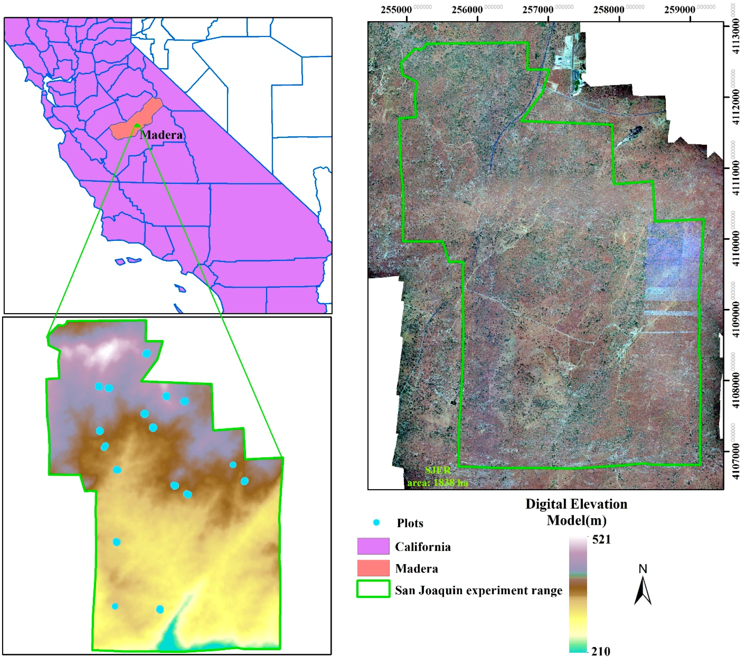
2.1. Study Site

Our study site is an ecosystem research experimental area, San Joaquin Experimental Range (SJER, UTM Zone 11N, Easting 257,600, Northing 4,109,300), which is situated in the foothills of Sierra Nevada Mountains and about 32 km north of Fresno, California (Figure 1). Within in the SJER, the vegetation is mainly composed of interior live oak (Quercus wislizeni), blue oak (Quercus douglasii), gray pine (Pinus sabiniana) and scattered shrubs with a nearly continuous cover of herbaceous plants. The whole area is characterized by the complex topography including coarse, large hills and valleys with elevation ranging from 210 to 521 m above sea level with a mean elevation of 366 m.

2.2. Data

2.2.1. LiDAR Data

FW LiDAR data of the study site were acquired during leaf-on season in June 2013 with an Optech Gemini instrument flying at approximately 1000 m above the ground level. The flight campaign was conducted by the National Ecological Observatory Network (NEON) Airborne Observation Platform, which provided FW LiDAR data with a 0.8 m diameter footprint and a spacing of about 0.524 m in the across-track direction and 0.5 m in the along-track direction. Compared to DR LiDAR data, the reported absolute range and vertical accuracies of FW LiDAR are 0.06–0.28 m and 0.15 m, respectively. The entire study area was covered by two perpendicular direction flight lines, with 12 and 19 flight lines in an east-west direction and north-south direction, respectively. Major technical specifications of the flight campaign have been reported in in the study of Zhou et al. [34].
In this study, two aspects of waveform related information were used: a return pulse with 500 time bins and corresponding reference geolocations. The temporal resolution of the return pulse is 1 ns (0.15 m) and zero-padding is applied to non-recorded values of the return pulse to keep the length of waveforms constant. For the reference geolocation of the corresponding waveform, eight basic geolocation information attributes associated with the waveform were obtained. Specifically, the attributes consist of the Easting of first return x0 (m), the Northing of first return y0 (m), the height of first return z0 (m), the pulse direction vectors (dx (m), dy (m) and dz (m)), the outgoing pulse reference bin location (leading edge 50% point of the outgoing pulse) and first return reference bin location (leading edge 50% point of the first return).

2.2.2. Reference Data
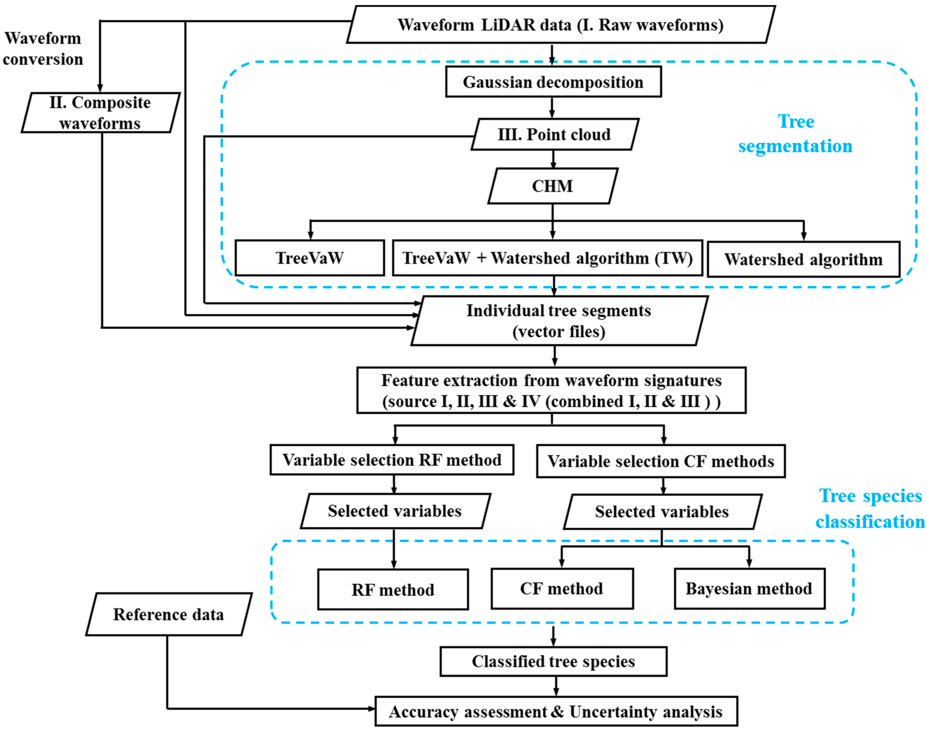
Field-measured data were collected across 17 plots in the study site during June 2013. An overview of the plots is displayed in Figure 1 with blue points. The locations of the plots were established by the NEON’s Field Sentinel Unit for measuring long-term plant, insect and soil related properties. According to the protocol of the NEON Terrestrial Observation System, the size of the plot is a square region with 20 × 20 m. A various number of trees were measured in each plot and in total 181 trees and shrubs (60 for the gray pine, 39 for the blue oak, 58 for the interior live oak and 24 for shrubs) were observed (Table 1). Several key vegetation structure variables were recorded and only locations (Eating and Northing) and tree species were used in this study.

2.3. Methods

The first step of automated tree species classification using LiDAR data is to segment individual tree crowns. Although exploring the capability of FW LiDAR data to segment trees is an important research area, it is not the major focus of this study. For the completeness of the methodology, we briefly described the process of the tree segmentation in Section 2.3.2. Previous studies have demonstrated that descriptive metrics can be extracted from the point cloud through waveform decomposition [3,18], raw waveforms [35] and composite waveforms [23]. However, it is unclear which source of metrics is more useful for characterizing vegetation such as tree species discrimination. Therefore, we extracted variables from these three sources and conducted a feature selection process within each individual source and all combined variables using RF and CF methods. Subsequently, the Bayesian, RF and CF methods were adopted to investigate the capability of FW LiDAR data alone on tree species identification using selected metrics from the feature selection step. An overview of the major steps for tree species classification using FW LiDAR data is shown in Figure 2.

2.3.1. Waveform Decomposition

As part of the preprocessing step of tree segmentation and metrics extraction, we first applied the Gaussian decomposition (Equation (1)) for waveforms to obtain a point cloud as described in our previous study [34]. The present study will not go into details of how the point cloud is obtained, whereas major steps of the procedure are the preprocessing of waveforms, the fitting waveform with a mixture of Gaussian functions and geolocation transformation. Once we obtained the point cloud, we employed LAStools [36] to classify ground points with lasground and then generated a CHM with 1 m resolution using the remaining non-ground points with las2dem and lasgrid. Simultaneously, the echo width ( δ i ) and amplitude ( A i ) of each waveform were derived for subsequent metrics extraction from the point cloud.
f ( x ) = i = 1 n A i exp ( ( x u i ) 2 2 δ i 2 )
where x is the index of time bin (1, 2, …, wl (the length of the waveform)), n is the number of Gaussian components, A i is the amplitude of peak at ith waveform component, δ i   is the standard deviation of ith waveform component and u i is the time location of the peak at ith waveform component.

2.3.2. Tree Segmentation

We first explored two commonly used algorithms including the variable window filter [7] and watershed algorithms [11] to segment tree crowns using the CHM derived from the waveform decomposition. TreeVaW uses an adaptive local-maxima filtering approach to detect treetops of individual trees and then attempts to estimate the crown size by assuming circular crowns around tree tops. The variable window filter was implemented through the TreeVaw package to identify tree tops and then measure crown width [37] as shown in Figure 3a. However, individual tree crown geometry was not well delineated since the shape of tree crowns is not always circular in the real-world. To reduce the bias caused by tree crown segments that could significantly affect the accuracy of extracted metrics, the watershed algorithm was employed to delineate individual tree crowns (Figure 3b). The geometries of individual tree segments are more representative of shapes of real individual tree crowns, while over-segmentation (green circles) is obviously observed with the watershed algorithm (Figure 3b) as compared to tree tops identified by TreeVaW. Therefore, we developed the third method, named TW, by integrating the TreeVaW adaptive filtering algorithm with the marker-controlled watershed segmentation algorithm [11], which is a variant of the watershed algorithm, to conduct individual tree detection and crown delineation to overcome the problems of the above two methods. According to our observations, some detected tree tops were close to each other which resulted in over-segmentation in tree crown delineation. Thus, we combined detected tree tops within 5.7 m (within 2 grid cells) to obtain final tree tops. The whole process was implemented in R [38] with the aid of the ForestTools package [39]. The marker-controlled segmentation algorithm delineated tree crowns based on the tree tops we identified in the above steps. The function in Table 2 refers to the linear relationship the user inputs into TreeVaW settings to control the adaptive filtering process. This function is based on the relationship between the height of trees and their crown size and can be derived from known species allometrics, from field measurements of tree height and crown size, or from user-derived point-cloud measurements of trees in the dataset. In this study, the relationship between tree height and crown width and the threshold of combining tree tops were determined by sampling trees in the dataset as visible on-screen in the point cloud and then refined with a trial-and-error method. In this section, we focused on describing the process conceptually and thus presented less details of algorithmic developments. More information on the watershed method implementation can be found in the study of Beucher and Meyer [40]. Key parameters used for identifying tree tops were summarized in Table 2.
To evaluate the accuracy of tree segmentation, we generated a 2 m buffer around the position of each field-measured tree top and compared these buffers to the delineated tree tops. Once a detected tree top was present in the buffer, we assumed the tree was correctly detected, otherwise, it would be treated as “false detected tree.” If more than one detected tree top was present in the reference tree buffer, it was assumed as an over-segmented tree top. The nearest detected tree top was kept for subsequent feature extraction and tree species classification in the over-segmentation condition.

2.3.3. Feature Extraction from Waveform Signatures

To preserve a plethora of original information from FW LiDAR data and improve the efficiency of FW LiDAR data in statistical models, we derived per-tree waveform signatures. The waveform signature at individual tree level is the aggregated laser energy profile along the height. To combine waveforms intersecting an individual tree crown area, we used two sources: (1) raw waveforms (Raw, I) and (2) composite waveforms (Composite, II) which are converted from raw waveforms through the voxelization process [22]. A third source to derive per-tree statistics is by using the waveform-based point cloud after Gaussian decomposition (Decomposition, III).
For raw waveforms, we first selected waveforms that fell into the delineated tree crowns and filtered out waveforms with one peak to reduce the bias of tree crown segments and to ensure waveforms selected were vegetation-related. Within each tree crown, we averaged the metrics extracted from individual waveforms, which have been successfully applied for characterizing vegetation, such as the height of median energy (HOME), the roughness of outermost canopy (ROUGH), the number of peaks (NP), the total return waveform energy (E), the waveform distance (WD), the median energy height ratio (MEHR), the front slope angle (FS) [21,22,23], the height of 50% total waveform energy (HOHE) and the half energy height ratio (HEHR). The average and standard deviation of these metrics were ultimately obtained as the model inputs. In addition, we averaged intensities from selected raw waveforms within each delineated tree crown based on the time bin and absolute height and obtained the accumulative waveform (AWF) for each individual segment as shown in Figure 3c. The integral of these two AWFs, the integral of vegetation (3 m above ground) and the ratio between the integral of vegetation (VegI, 3 m above ground), the integral of ground (GI) and the ratio between the integral of vegetation and the additive integral of vegetation and ground parts (RvegT) [35] were also calculated. Overall, we extracted 56 metrics to characterize vegetation from the raw waveform source.
With respect to composite waveforms, previous studies have demonstrated that off-nadir angle of flights indirectly alters the absolute vertical distribution of reflected intensities and results in the stretchiness or tilt of waveforms [22]. To reduce its possible impact on the characterization of internal structures of vegetation using FW LiDAR data, an approach similar to that of Hermosilla et al. [22] was adopted to convert raw waveforms to composite waveforms with the voxel resolution of 0.8 × 0.8 × 0.15 m. The reason for using this resolution was that the footprint of FW LiDAR is approximately 0.8 m and the vertical resolution of raw waveform is 0.15 m. Specifically, we partitioned the spatially-located raw waveform signals into the voxel space defined above and employed the mean intensity of waveform signal(s) within each voxel to represent the waveform intensity of the composite waveform. Likewise, we applied the same procedures of retrieving metrics from raw waveforms to extract variables from composite waveforms. To sum, there were 46 variables were derived from the composite waveform source.
Regarding the metrics from the point cloud, we conducted waveform decomposition of these selected waveforms and then summarized the average, standard deviation and maximum of the amplitude, echo width and peak time bins for each tree crown segments. Additionally, the first peak and last peaks’ average amplitude and echo width were also generated. In total, 18 variables were generated from the point cloud source. The main variables extracted from waveform and point cloud are summarized in Table 3 and a detailed description of all metrics from the three sources is demonstrated in Table A1.

2.3.4. Feature Selection

Generally, dimension reduction techniques such as principal component analysis with statistical analysis are adopted to deal with a large number of variables. However, the effect of individual variables cannot be directly identified due to original variables being projected into a reduced set of components after an orthogonal transformation [26]. Recently, a growing number of studies have highlighted the effectiveness of the RF algorithm to reduce the dimension of input variables for subsequent classification [19,23]. RF [41] is one of several popular ensemble learning methods based on the principle of recursive partitioning which could overcome the instability of individual classification trees induced by subtle changes of training samples. Originally, the variable importance is measured by merely counting the occurrence of each variable in all individual trees. As time evolves, the average splitting improvement of each variable in all individual trees is employed to assess the variable importance, such as the Gini importance [26]. A more intuitive variable importance measure in the RF is the permutation accuracy importance, which is calculated as the mean difference in prediction accuracy before and after permuting variable Xj over all trees. This measure has been shown to be a reliable criterion for quantifying the variable importance of uncorrelated predictors. However, the traditional permutation accuracy importance is prone to bring about potential bias for variable selection when predictors vary in scales or the number of categories [27]. Additionally, the RF is likely to divide the importance amongst the correlated predictors. Consequently, none of these predictors may be significant for the model. Actually, the permutation results of the RF approach reflect independence between Xj and both Y and the remaining predictor variables Z (X1,… Xj−1, Xj+1,…, Xp) instead of only the importance of Xj in predicting the response Y. Thus, we introduced a variant of permutation importance of the RF algorithm, conditional importance, to mitigate possible bias and avoid the impact of correlated variables for the feature selection in this study.
In contrast to the permutation importance in the RF, the conditional importance is achieved through an unbiased classification tree generated by subsampling without replacement method instead of bootstrap sampling. Additionally, the hypothesis of conditional importance measure is that Xj and Y are independent given the correlation structure between Xj and Z inherent in the data set. Within the framework of the conditional permutation, Xj is permuted only in a discretized permutation grid rather than the whole dataset. The grid is determined by the partitions derived from the model fitting or cut points of empirical correlations between Xj and Z [27]. In the implementation, variables Z whose correlation with Xj meets the condition 1 − p-value > 0.2 are used for conditioning. For each grid, the out of bag (OOB) error prediction accuracy is measured in one tree after permuting the values of Xj. Similar to the permutation importance, the conditional importance of Xj is the average prediction accuracy of all classification trees.
We employed both permutation importance and conditional importance to conduct the feature selection from three individual sources (I, II & III) and all combined variables (Combined, IV) with a total of 120 FW metrics. Prior to calculating the relative importance of variables, we excluded variables with importance (directly from the RF and CF methods) less than zero. The rationale behind this is that the importance of irrelevant variables changes randomly around zero [26]. To minimize the overfitting of the model and make it more generalized, nine candidate variables whose relative importance are larger than 1.5 with different characteristics were selected as the input for subsequent Bayesian classification using combined variables. According to the rank of the variable importance in each individual source, nine most significant variables were also identified in each source for subsequent tree species classification to ensure the consistency of model input and further increase comparability among models.

2.3.5. Tree Species Classification

To comprehensively explore the capability of FW LiDAR data on the tree species discrimination, three methods including the RF, CF and Bayesian inference were proposed to examine the usefulness of metrics and compare methods’ prediction performances.

Random Forests and Conditional Inference Forests

Not only can the RF measure the importance of variables but it is also widely used for classification and regression. The bootstrap method is adopted to resample part of the original dataset as training data to generate n classification or regression trees. For each tree, m variables out of p variables (total) were selected randomly to conduct classification or regression. When a new data X is present, we aggregate predictions of the n trees’ results using the new data. Suppose that the ensemble of trees is   { T i } 1 n , for regression, p(X) =   1 n 1 n T i ( X ) ; for classification, p(X) = majority votes { T i ( X ) } 1 n . Within every tree, the OOB error is calculated using the remaining data from the original data as the OOB dataset.
Compared to the RF classifier, there are two main differences for the CF classifier: resampling method and permutation scheme as we have described in the Section 2.3.4. The thrust for employing the CF method was to reduce the bias during variable selection in the RF method and provide a thorough understanding of the variable selection in a stringent statistical framework.
In this study, we set the number of trees to 10,000 for both methods and aimed to compare their performances with the same setting. Nine metrics were chosen for the final classification and other irrelevant variables were discarded. Through the experiment, incorporating more variables did not decrease the OOB error.

Bayesian Inference

The motivation for introducing the BMLR method in this study was to better understand the uncertainty of the classification and provide a new insight into the multinomial regression on tree species identification using FW LiDAR data. There are various models to conduct regression analysis for the multinomial data, such as the multinomial logit model, random utility model and multinomial probit model [42]. Here, we employed the softmax regression model [43] to formulate the tree species prediction model to represent the categorical distribution.
We assume that Y follows a multinomial distribution with sample size N and parameter vector p. yi is one of s unordered categories, labeled by   k = { 1 , , s } . When s is 2, the softmax model reduces to the logistic regression model.
We are interested in the model probability of categories 1 to s. Thus, yi takes value from 1 to s according to the covariate information. For outcome k, the underlying linear propensity λ k   is denoted as:
λ k = x i β k
The softmax model can be formulated as follows:
P ( y i = k | β 1 , ,   β s ) = exp ( x i β k ) m = 1 s exp ( x i β m )
where β 1 , ,   β s are category specific unknown regression coefficient vectors and each vector contains q unknown parameters (q − 1 unknown parameters for corresponding variables and one for the intercept). x i is a row vector with covariates (1 × q) which are not category specific and includes 1 for the intercept. Generally, category 1 is adopted as a baseline category with β1 = 0.
Subsequently, the Bayesian approach was pursued and prior distributions were assigned for all regression coefficients. There are two main options to specify priors, non-informative priors and empirical priors. The non-informative priors indicate that assigning equal probabilities to all possible values of parameter space which can reduce the effect of prior information on the posterior distribution. For the empirical priors, a normal distribution N (b0, S0) roughly derived from data can be assigned to these unknown regression parameters. In this study, empirical priors for these parameters (b0) were derived from multinomial logistic regression with a large standard deviation S0 = 4, which can be assumed as weak informative priors. According to the Bayes’ rule, the posterior distribution of β can be written as:
P ( β 1 , ,   β s | y )   p ( β 1 ) p ( β s ) i = 1 n [ exp ( x i β k ) ] y i m = 1 s exp ( x i β m )
In our case, we have three tree species (gray pine, interior live oak and blue oak) and one shrub species and either one can be a category response (y). The field-measured data were split into training and testing data using a random selection procedure. To mitigate the impact of this random selection procedure and different proportions of testing data on the variability of accuracy, we tested different proportions of testing data ranging from 0.15 to 0.35 with the interval of 0.025 on the model accuracy. The corresponding remaining proportion of data were used as training data to build models.
For the RF and CF methods, the OOB prediction accuracy with training data and confusion matrix derived from testing data were employed to quantify the prediction accuracy of tree species discrimination. Prior to deriving the Bayesian model inference, the model convergence was verified with the potential reduction factor, named Rhat ( R ^ ), which is a criterion to measure how well the Markov Chains are mixing and moving around the parameter space [44]. Generally, R ^ is expected to be close to 1; otherwise, a longer chain is necessary to be run or more reasonable priors should be assigned to ensure that the chain reaches the stationary state. As opposed to results of the RF and CF methods, the BMLR method can generate probability distributions belonging to four tree species for each delineated segment. The tree species of an individual tree segment was determined with the largest probability among these four estimated probabilities. Once the model was built, the testing data were used to assess the accuracy of the tree species discrimination. The above described BMLR method was implemented in R using the brms package [45].

3. Results

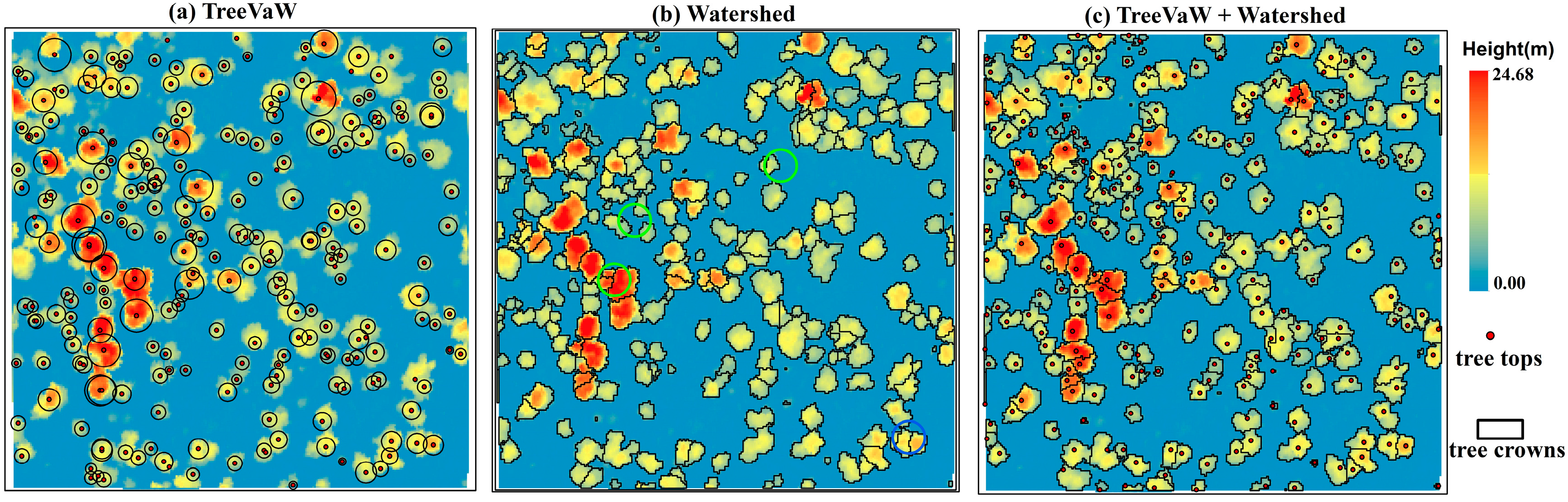
3.1. Tree Segmentation

Three approaches including TreeVaW, watershed segmentation and TW segmentation were employed to conduct the tree segmentation in the SJER study site (Figure 3). The major difference of segmentation results between the TreeVaW and the other two approaches was the shapes of individually delineated tree crowns. It is worthy to note that some TreeVaW-identified tree tops had no delineated tree crowns in the border of the example region, which happens when the software cannot fit a mathematical spline over the tree crown profile. The detected tree positions of these three approaches were indistinguishable, while the watershed approach was prone to over segment individual tree crowns (blue circles).
To further illustrate segmentation results over the whole region, a quantitative evaluation of these approaches is presented in Table 4. Results of the tree segmentation demonstrated that the watershed approach outperformed the other two approaches at tree detection, while its corresponding over-segmentation rate was the highest among these methods. In contrast, results of TreeVaW showed the lowest over-segmentation rate with the highest false detection rate. These results, of course, were not surprising: it is natural to expect higher accuracy of tree detection when more trees were delineated with a higher probability of over-segmentation. Through the TW approach, the bias caused by the over-segmentation can be reduced with lower over segmentation rate and decent tree detection rate (~90%). Thus, the segmentation results from the TW approach were adopted to conduct subsequent feature extraction.

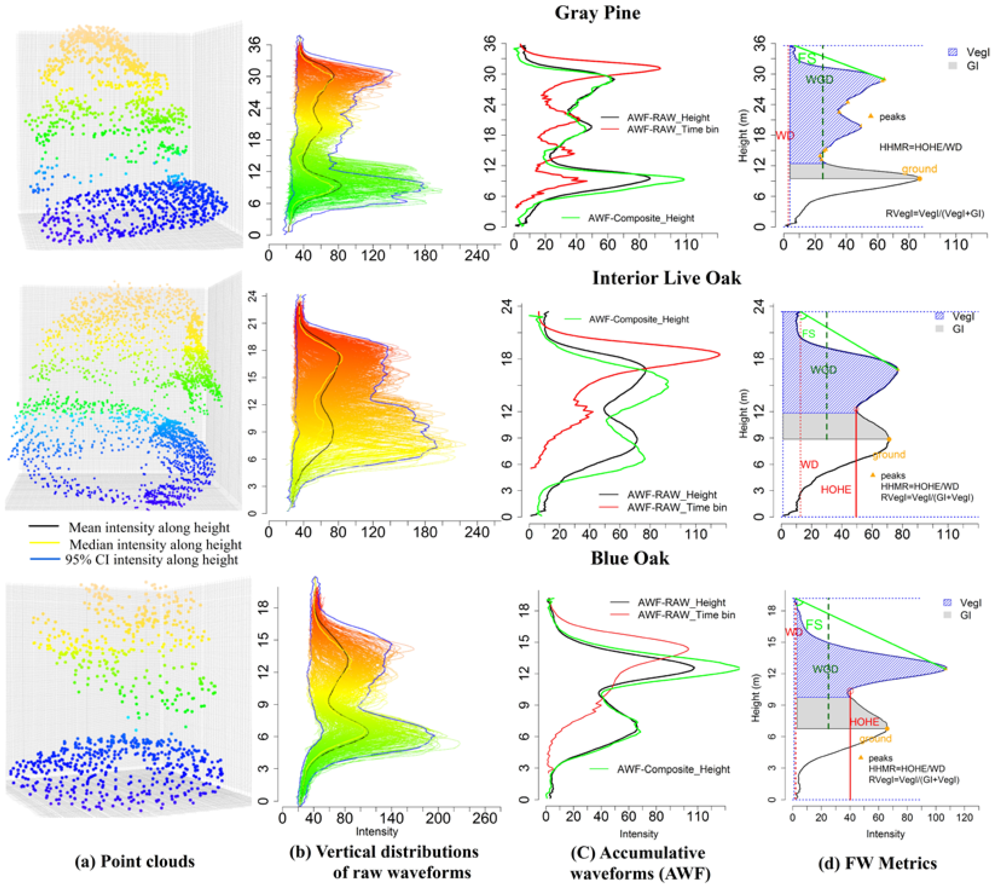
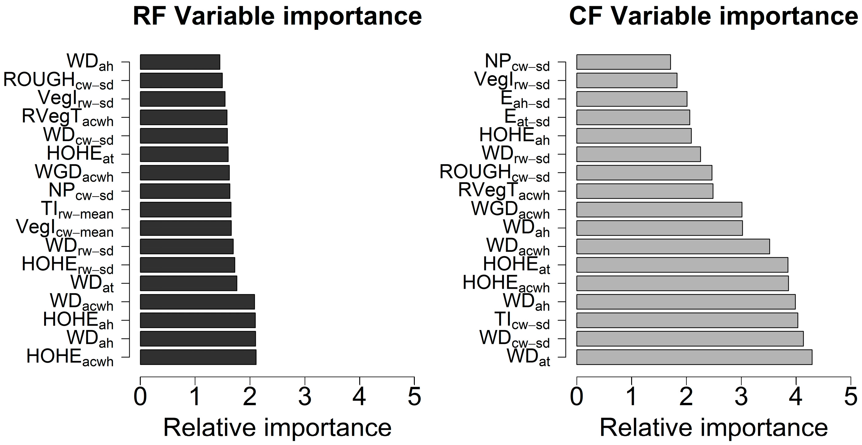
3.2. Feature Extraction & Selection

To visually display the pattern between tree species and waveform metrics from various sources, we demonstrate waveform signatures for three representative trees (Figure 4). It is evident that the terrain and tree crown shapes are significantly different among these three tree species for the waveform-based point cloud after the Gaussian decomposition (Figure 4a). As shown in Figure 4b, the intensity distributions along the height for every individual waveform within an individual tree boundary are demonstrated. A common intensity distribution pattern for these three tree species emerged from Figure 4b showing that more energy was concentrated in the upper part and lower part of these tree species. The 95% confidence intervals, median and mean of intensity were plotted against the height to display an overview of the intensity distribution of waveforms for different tree species. To present summary statistics of all waveforms within one tree segment, the AWF along the time bin (red line) and height (black line) for each tree species are generated as shown in Figure 4c. As expected, the length of the time bin based AWF was shorter than the height based AWF. The length difference of these two AWFs was strongly correlated with the slope of the terrain where the tree located. Compared to height based AWF from raw waveform (black line), the counterpart derived from composite waveform (green dash line) almost shared the same energy distribution.
An interesting observation that emerged from the time bin based AWF comparison was that there was a subtle difference between interior live oak and blue oak while the latter had more energy distributed at the bottom part. However, their difference, with respect to the gray pine, was evident in terms of the number of peaks and energy distribution along the height. These differences render a prospect for tree species classification with these waveform metrics. Thus, we demonstrated several waveform metrics extracted from the AWF along the height as an example in Figure 4d. It was evident that the WD, VegI, FS and RVegT varied across different tree species from the visualization perspective.
To quantitatively identify influential waveform metrics for the tree species classification, the waveform metrics ranking and selection were conducted through the RF and CF methods. Figure 5 depicts the comparison of variable importance using the CF and RF methods with 10,000 random forest trees using combined variables. For illustration purposes, we presented the most important 17 variables identified by the CF method with their relative importance and corresponding importance derived from the RF method to exhibit the comparison of variable importance results. Compared to the CF method, relative variables’ importance of RF method was smaller and more likely to be evenly distributed. Consequently, it was more difficult to recognize significant variables, which undoubtedly mitigate the capacity of the RF method for measuring variables’ importance. It was observed that the WDs and HOHE extracted from different sources were more significant than other variables for both approaches. Additionally, the WGD, RVegT, FS, VegI and NP were also highlighted as important variables for classifying tree species. Interestingly, more variables derived from the AWF were found to be significant predictors than the average of variables from individual waveforms within one segment for the tree species discrimination. In terms of sources of variables, composite waveforms were more representative than other sources. This result is also verified by investigating accuracy assessment of tree species classification using variables from individual sources.
To mitigate the overfitting caused by highly correlated variables and avoid the replication of the same variables from different sources, WDat, WDcw-sd, TIcw-sd, HOHEacwh, WGDah, RVegTacwh, Eat-sd, VegIrw-sd and NPcw-sd were used for subsequent Bayesian inference for the tree species classification. Here, the subscript represents the variables’ source and statistical features (mean, max and standard deviation). For example, WDat denotes the WD from AWF of one tree segment along the time bins (at); WDcw-sd denotes that standard deviation of WDs derived from individual composite waveforms (cw) of one tree segment; WDrw-sd denotes that standard deviation of WDs derived from individual raw waveforms (rw) of one tree segment. Detailed descriptions of these variables can be found in Table A1.

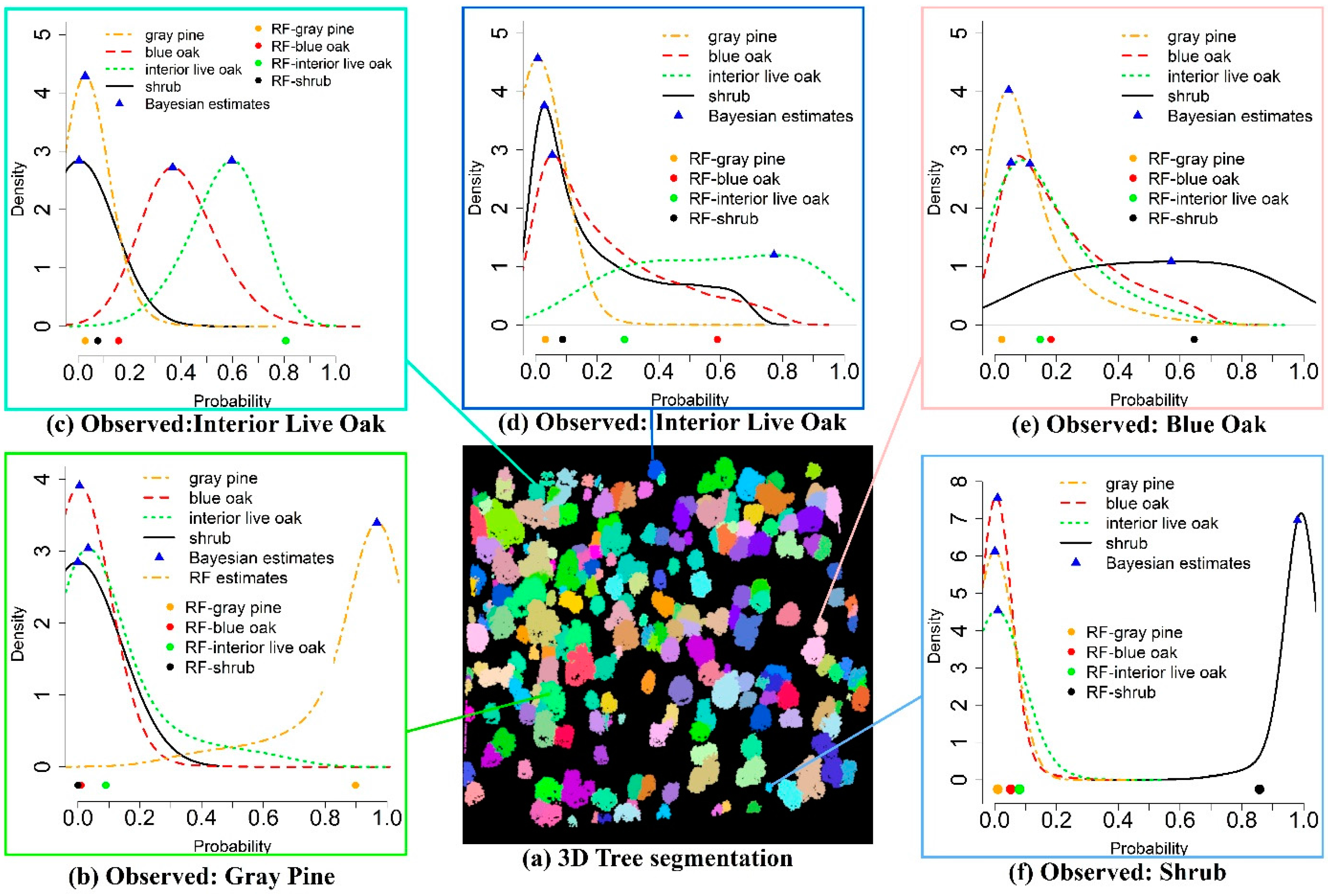
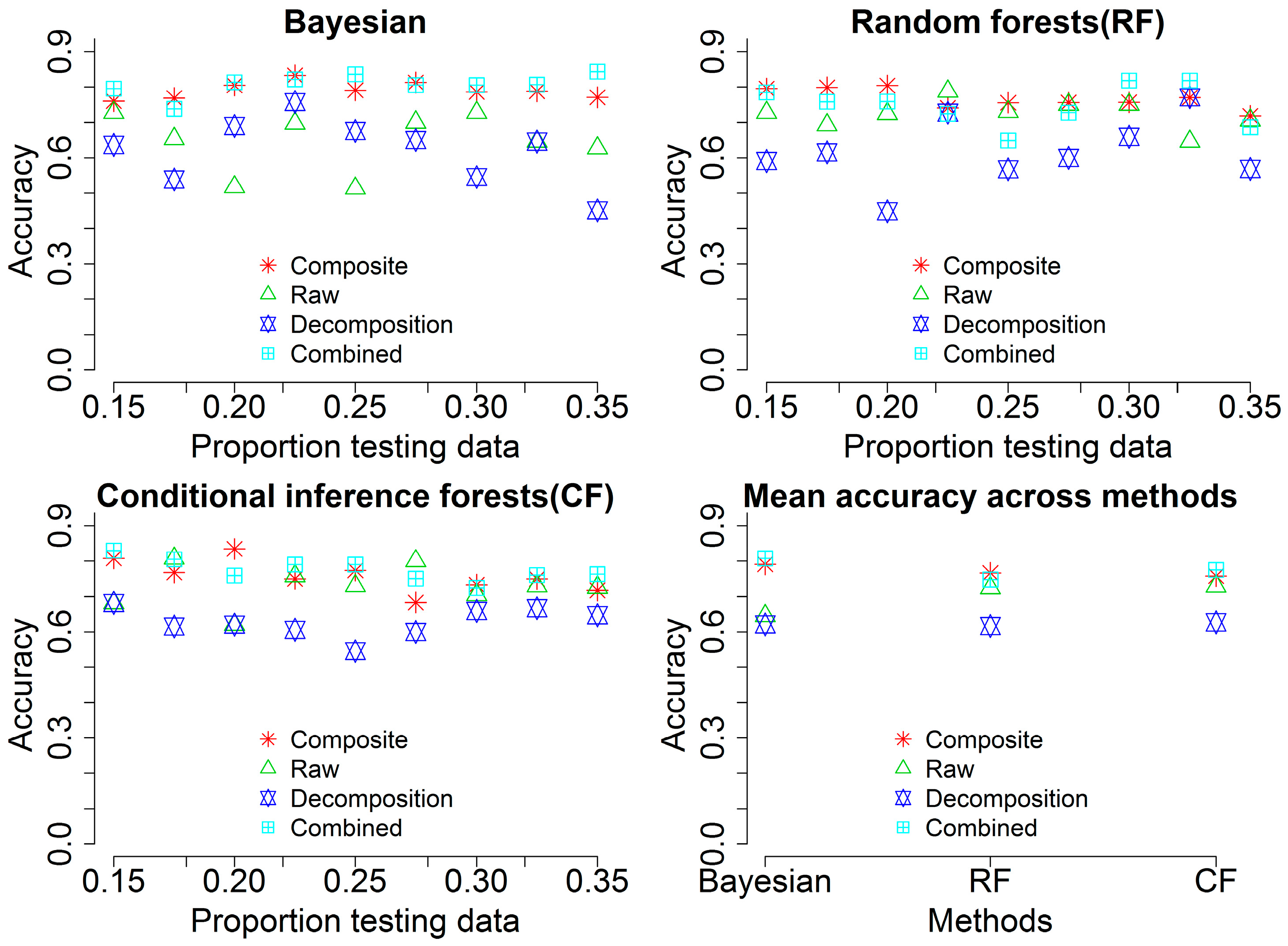
3.3. Classification Results

Figure 6 exemplifies the classification results using the RF and BMLR methods with five individual trees in a subset region. The CF method generated almost the same result as the RF method for these five trees, thus CF estimates were not plotted. In Figure 6a, the clusters with different colors represent delineated individual tree segments with the TW method. The other five subplots were the five field measured trees with corresponding classification results using the RF (dots) and BMLR methods with probability distributions for possible tree species (blue triangles represent the mode of the probability, y-axis represents the probability differential (the probability per unit, such as 0.01)). Compared to the field-measured data, Figure 6b,c,f were correctly classified as gray pine, interior live oak and shrub, respectively, using both the RF and BMLR methods. With the RF method, four estimated probabilities belonging to possible corresponding four tree species for an individual tree were generated and this tree is classified as gray pine with the largest probability (Figure 6b). As opposed to one estimated probability for each possible tree species using the RF method, the BMLR method could generate four probability distributions for these four possible tree species and the tree species of one tree was determined by comparing their probability distributions. For example, it is evident that trees are classified as gray pine and shrub with a compact probability distribution and high posterior mode probability (>0.92) in Figure 6b,f, respectively, both of which are higher than corresponding point estimates obtained from the RF method. The RF method is also possible to correctly identify tree species with a higher probability than the BMLR method as shown in Figure 6c. In Figure 6c, the tree is correctly identified as interior live oak for the RF method with a high probability, while the tree could be classified as blue oak or interior live oak in terms of probability distributions with the BMLR method. Nevertheless, the tree is more probable to belong to interior live oak with a slightly higher probability when comparing the modes of probability distributions for both candidate tree species. Figure 6d illustrates that a tree is correctly classified as interior live oak using the BMLR method according to its stretched probability distribution but it is misclassified as blue oak with the RF method. It is also possible that the discrimination power of both methods fails when they are confronted with complex tree segments or wrong segmented tree crowns, such as in Figure 6e.
To achieve a full comparison of classification performances from different sources, we summarized overall accuracies with the three methods in Figure 7. Classification results using different testing proportion data show that there is a subtle change of the overall accuracies when the input data coming from composite waveforms (Composite, cyan square plus) and combined variables (Combined, red star). Contrarily, the other two sources including raw waveforms (Raw, green triangle) and point cloud (Decomposition, blue triangles up and down) demonstrate larger variance of overall accuracies across different testing proportion data. Generally, the overall accuracy from combined variables is higher than the other three sources while there is no significant difference of the overall accuracy between the combined variables and composite waveforms in most of cases. The mean overall accuracy among the three methods shared similar pattern with the individual sources (Combined ≥ Composite > Raw > Decomposition) and the BMLR method outperforms the other two methods.
An example of the classification results with the RF and CF methods using all combined variables was summarized in a confusion matrix to quantitatively show individual tree species identification accuracy when the testing proportion was 0.2. The prediction accuracy of the RF and CF methods can be measured with the training data (OOB error) and testing data, therefore we separated the results into Table 5 and Table 6. Overall, the most distinguishable species were the gray pine and shrub with a decent classification accuracy, both of which were differentiated from the other two tree species. The least accurate tree species was the blue oak since it was easy to be misidentified as the interior live oak when taking the second column of tables into account. There was a subtle difference in the classification accuracy for the RF and CF methods in terms of the overall accuracy using the testing data, while the RF outperformed the CF from the perceptive of OOB error using the training data. A comparison of different methods using the testing data showed that the BMLR method was superior to other two methods with higher overall accuracy and Kappa coefficient.
Furthermore, uncertainty of classification accuracy is also generated in a probabilistic sense with the BMLR method, rather than a single estimate as shown in Figure 8. According to Figure 8, the 95% credible interval for the overall classification accuracy is approximately [0.52, 0.87]. Without doubt, this result is more informative than the counterpart such as the results from the RF and CF methods with only one estimate of classification accuracy.

4. Discussion

4.1. Tree Segmentation

There are two major steps for the tree segmentation: the tree top detection and tree crown delineation. Based on experimental results, watershed algorithm alone is prone to face the over-segmentation problem at the tree top detection step. By contrast, the method implemented in the TreeVaW is more likely to give an unreasonable delineation of tree crowns. With the TW algorithm, these two flaws can be mitigated and consequently improve the accuracy of the tree crown delineation. The performance of the tree crown segmentation, on which subsequent accurate extraction of waveform metrics depends on, may be of greater significance. One salient reason is that our waveform metrics are derived from delineated individual tree crowns and inaccurate delineated tree crowns undoubtedly result in false waveform metrics and less precise tree species classification.

4.2. Individual Trees’ Waveform Signatures

It is evident that structures of the three tree species are different through visually comparing point clouds after the Gaussian decomposition (Figure 4a). Additionally, the vertical intensity distribution along the height for waveforms within one segment highlights the ground and canopy parts with concentrated energy distribution. These two intercepted surfaces with backscattering render significant insights into tree height measurement and tree species characterization. In addition, higher amplitudes and intensities are prone to occur for the blue oak and interior live oak compared to the gray pine, while the gray pine has a larger number of echoes with longer pulse line (Figure 4c). What these trees share is that the first echo corresponding to the canopy part has a greater amplitude than those of subsequent echoes. A possible explanation for this may be that transmission losses are occurring along the pulse penetrating the tree canopy: the deeper the pulse transmits, the less the energy is left. The internal structure of the blue oak in Figure 4a is sparsely branched which may contribute to the more energy reaching the ground part and its second amplitude is almost the same as the first amplitude. In addition, the comparisons of the AWF along the time bin and height bin can inform whether the topography of the tree’s location is a slope or not, because the AWF along the time bin did not take the height information into account with the same starting bin and thus will make the length of its AWF shorter than the AWF along the height bin when a slope is present.

4.3. Waveform Metrics and Feature Selection

This study expands on previous work in exploring waveform metrics for vegetation characterization using FW LiDAR data and introduces the concept of waveform signature. We examine waveform metrics from three individual sources and conduct rank comparisons among these variables to identify which source of waveform metrics is more preferred for characterizing tree species. The raw waveform with the off-nadir angle could potentially provide more detailed structural information of vegetation, while it is possible to alter the vertical distribution of energy distribution and give rise to false information of representative objects along the height. Contrarily, composite waveforms overcome this problem by reassigning intensity into the absolute height bins. Results demonstrate that waveform metrics from composite waveforms are more informative than raw waveforms and point clouds (Figure 7). This may suggest that more attention should be paid to composite waveforms when the absolute vertical related information is used. Compared to the point cloud from DR LiDAR data, the waveform-based point cloud is generally more dense and informative [17,34]. In the present study, waveform metrics from raw and composite waveforms have demonstrated that both are capable of providing a more promising prospect of potential applications such as tree species identification than waveform-based point cloud data Therefore, this result indirectly confirms that waveform LiDAR data are more useful for vegetation characterization than DR LiDAR data. Another important finding about variable importance is that the AWF for each individual tree segment contains enough information for characterizing features of different tree species. Therefore, the metrics derived from the AWF can be considered as a proxy for further vegetation characterization or biomass mapping without averaging extracted information from the individual waveforms within a segment.
The RF variable importance measures have been adopted as a sensible means for variable selection in many remote sensing applications [23,46]. Built upon the RF method, we introduced an alternative method, the CF, to explore their usefulness in variable selection. From a statistical perspective, both methods are capable of dealing with high dimensional datasets and solving “small n large p” problem with similar results (Figure 5). However, a closer examination of the variable importance suggests that the RF method is prone to be biased for measuring the variable importance since the permutation process implemented in the RF method favors correlated predictor variables [47] and divides importance among these predictors. Consequently, an evenly distributed importance for many variables are generated as shown in Figure 5. As expected, the CF method produces more reasonable variable ranking results and clearly distinguishes variables’ importance by using the subsampling without replacement strategies and a conditional inference framework.
With regard to individual variables, the WD, TI, HOHE, WGD, RVegT, FS and ROUGH are identified as significant factors for tree species classification using both the RF and CF methods in this study. In accordance with previous studies [23,35], the WD, HOHE and WGD have a stronger capacity for characterizing different tree species, which are related to the height or crown height of individual trees. Essentially, these results are also consistent with the height characteristics of these tree species, with significant differences in the tree heights among these tree species and shrub. More specifically, within our research area, the height of gray pine is generally the highest and the shrub has the lowest height. As demonstrated in Figure 4d, the integral of the waveform (TI) and the ratio between vegetation part and the whole waveform (RvegT) vary among different tree species and a higher percentage of the vegetation integral is expected in the gray pine since more energy is retained in the vegetation part with longer pulse lines and less energy reaches the ground.
It is worthy to note that variability of outcome for the variable selection process may exist using the RF and CF methods, since the importance of variables is derived from a random permutation of predictor vectors [26]. However, variables or the method proposed in this study may potentially serve as a practical guideline to identify significant metrics and infer characteristics of interest (e.g., volume, biomass, carbon) using FW LiDAR data.

4.4. Tree Species Classification and Uncertainty

This study exemplifies the use of advanced statistical methods (the RF, CF and Bayesian) to explore a wealth of information contained in FW LiDAR data for discriminating tree species. In practice, various sources of randomness in the RF and CF could contribute to the discrepancy or instability of prediction accuracy: (1) subsampling process which randomly draws sub-data samples from the whole dataset and (2) an individual tree building process which randomly draws part of variables from all variables [26]. To obtain a reliable accuracy assessment, we set “ntrees” of 10,000 and “mtry” of nine in both models. Table 5 and Table 6 demonstrate results with setting the same random seed at the beginning of running to ensure the replication of results. The results of OOB error using the training data demonstrate that the prediction accuracy of the RF method is higher than the CF method. However, the CF method slightly outperforms the RF method when employing the testing data to evaluate the prediction accuracy. Both methods can generate acceptable results with a decent accuracy larger than 70%. It appears that the RF is superior to the CF method when we combined results from Table 5 and Table 6, while it is still arbitrary to judge the performances of these two methods only relying on the accuracy assessment using the result of a study area. The Analysis of variance (ANOVA) of different testing proportion results showed that there is no significant performance difference between the RF and CF methods. However, the ANOVA of overall accuracy results between the BMLR method and individual the RF or CF method suggested that the BMLR method is slightly outperformed other two methods with p-value smaller than 0.1 (the 90% confidence interval).
The statistical basis of the analysis for these two methods is built upon the frequentist inference. As an alternative, we applied a method based on Bayesian inference to conduct the tree species classification. As demonstrated in Figure 6, the BMLR method not only provides one estimate or probability for possible tree species, it also renders users to interpret results in a probabilistic sense for each tree. This interpretation is more intuitive through updating prior beliefs or probability of the tree species in response to new data and further gives us more confidence in the prediction results with predictive uncertainty. These advantages are more evident in dealing with the sophisticated tree species classification than simple classification (one tree species’ probability outstands among the other possible tree species). For instance, the tree species in Figure 6d is misclassified with the RF and CF methods while it has been correctly identified using the BMLR method with a flat posterior distribution. These three methods consistently perform well in simple classification examples such as in Figure 6b,f. In this study, the difference of the probability for one tree belonging to the blue oak and interior live oak is relatively small due to their similar physical characteristics such as the round tree crown and similar tree height. For the RF and CF methods, only one probability estimate is obtained for each possible tree species and the predicted tree species is identified with the largest probability. Any variance or uncertainty in tree crown delineation, variable extraction and model building steps undoubtedly contributes to misleading classification conclusions, especially for discriminating the blue oak and interior live oak. With the aid of the BMLR method, the overall accuracy may not be enhanced significantly but it can make the inference become more realistic with quantifiable predictive uncertainty (Figure 8). Simultaneously, the confidence about conclusion and uncertainty levels of results can be illustrated with the probability density functions. For example, compared with results of Figure 6d, a stronger belief of the trees belonging to the gray pine and shrub in Figure 6b,f, respectively, is guaranteed due to their more compact distributions.
The superior performance of the BMLR method is further substantiated with a higher overall accuracy than the other two methods (Figure 7). In essence, the RF and CF methods are more like “black-box” methods and they are developed in a less stringent statistical framework [26], both of which may lead to less predictive results than the BMLR method. Assuredly, more studies and applications of these methods or other methods should be exploited to further compare their performances in various applications and provide a more thorough understanding of how these methods can be practically utilized for real-world problems and when the caution should be exercised for result interpretation.
Surprisingly, these three methods all suffer from discriminating the blue oak from the interior live oak with relatively low accuracy. Various factors possibly contribute to the failure of methods including an inaccurate tree segmentation, an absence of the accurate field data and an insufficient number of waveform metrics. Specifically, our waveform LiDAR data were acquired in leaf-on season and crowns of neighboring trees are more likely to be overlaid. The blue oak and interior live oak share similar shape of tree crown and heights which undeniably reduces the success rate of tree segmentation and brings more challenges for subsequent tree species classification. The study of Yao et al. [18] also confirmed that the tree crown segmentation is more precise when the leaf-off season LiDAR data are used. It is anticipated that higher accuracy is obtained and more transparent vegetation structure is expected to be characterized by FW LiDAR data in leaf-off season. We envision a concomitant expansion of adopting advanced statistical methods such as the BMLR method for tackling complicated relationships between characteristics of interest (e.g., height, biomass, carbon) and remotely-sensed predictors and assisting result interpretation and decision making in real-world applications with advances of computational capacity and handy operational tools.

5. Conclusions

This study integrates an exhaustive set of waveform metrics from the waveform-based point cloud, raw waveforms and composite waveforms with machine learning (the RF and CF) and Bayesian methods to discriminate tree species using FW LiDAR data alone. We combine TreeVaW and watershed algorithms to derive more accurate individual tree segments, aiming to mitigate uncertainty and error brought into subsequent metrics extraction step. Classical machine learning methods such as the RF and CF demonstrate that they are powerful tools for coping with “small n large p” problems. Moreover, the CF method can overcome the possible bias of the RF method in measuring variable importance, which violates the implicit null hypothesis and favors correlated waveform metrics. Results of the variable importance suggest that composite waveforms provide more informative metrics than other sources which is consistent with overall accuracies of classification using data from different sources. Specifically, waveform metrics such as the WD, HOHE, WGD, RVegT, TI and ROUGH are highlighted as significant metrics to characterize tree species in our study. The combined variables from different sources do not significantly improve the tree species discrimination as compared to variables from composite waveforms. Tree species classification results show that the BMLR method achieves higher overall accuracy and Kappa coefficient as compared to the RF and CF methods. Additionally, the prediction uncertainty of each tree is also generated with the BMLR method, which permits the users to interpret results in a probabilistic sense without just relying on one estimated probability to construct decision rules to determine tree species. Furthermore, the uncertainty of accuracy for tree species classification provides a comprehensive overview of classification performance, which can assist to determine whether the classification accuracy reaches a particular standard and further guarantee users with more confidence to apply results for real-world tasks such as forest inventory. Certainly, the applied statistical methods need to be tested for various other forests and vegetation types. Further, it is worthy to note that one could have also fitted multinomial regression in a frequentist framework and that—at least in principle—RF could have been fitted in a Bayesian framework, as well. In addition, more efforts should be directed to exploit rich information contained in FW LiDAR for biomass and vegetation mapping.

Acknowledgments

We gratefully acknowledge the support from NSF Doctoral Dissertation Improvement Grant (DEB1702008) and NASA’s ICESat-2 SDT (Grant # NNX15AD02G). We also thank the National Ecological Observatory Network (NEON) for providing waveform LiDAR and field data. The open access publishing fees for this article have been covered by the Texas A&M University Open Access to Knowledge Fund (OAKFund), supported by the University Libraries and the Office of the Vice President for Research. Last but not least, we greatly appreciate the constructive comments from the three anonymous reviewers.

Author Contributions

Tan Zhou and Sorin C. Popescu designed and conceptualized the study. A. Michelle Lawing, Marian Eriksson and Bogdan Strambu gave comments and modified the manuscript. Paul C. Bürkner gave comments on the Bayesian method parts and provided feedback on the manuscript. All authors contributed to the editing of the manuscript.

Conflicts of Interest

The authors declare no conflict of interest.

Appendix A

Table A1. Summary of FW metrics from FW LiDAR data.
Waveform MetricsDefinition (Within an Individual Tree Segments)
Individual raw waveforms
AreaThe area of an individual tree crown segment
NPrw-meanThe average number of detected peaks for raw waveforms
NPrw-sdStandard deviation of NP
MaxPrwMaximum of NP
WDrw-meanThe average distance from waveform beginning to waveform ending using raw waveform
WDrw-sdStandard deviation of WDmean
HOMErw-meanThe average distance from height of median energy in waveforms to the ground
HOMErw-sdStandard deviation of HOMEmean
HTMRrw-meanThe average ration between HOHE and WD
HTMRrw-sdStandard deviation of HTMR
HOHErw-meanThe average distance from height of half energy in waveforms to the ground
HOHErw-sdStandard deviation of HOHE
HTHRrw-meanThe average ration between HOHE and WD
HTHRrw-sdStandard deviation of HTHR
FSrw-meanThe average vertical angle from waveform beginning to the first peak
FSrw-sdStandard deviation of FS
ROUGHrw-meanThe average distance form waveform beginning to the first peak
ROUGHrw-sdStandard deviation of ROUGH
TErw-meanThe average total energy of raw waveforms
MErw-meanThe average energy of each raw waveform
MaxIrw-meanAverage maximum intensity of all raw waveforms
TIrw-meanThe average integral of energy along height from waveform beginning to the ground
VegIrw-meanThe average integral of energy along height from waveform beginning to 3-m above ground
RVegTrw-meanThe average ratio between VegI and TI
MaxIrw-sdStandard deviation of maximum intensity
TIrw-sdStandard deviation of the integral of energy along height from waveform beginning to the ground
VegIrw-sdStandard deviation of the integral of energy along height from waveform beginning to 3-m above ground
RVegTrw-sdStandard deviation of the ratio between VegI and TI for all waveforms in the individual tree crown segment
Accumulative waveform along the time bin
NPatThe number of peaks in the time bin based accumulative waveform
WDatThe distance from waveform beginning to the ground in the time bin based accumulative waveform
HOMEatThe distance from height of median energy to ground in the time bin based accumulative waveform
HOHEatThe distance from height of half energy to ground in the time bin based accumulative waveform
HTMRatThe ration between HOMEat and WDat
HTHRatThe ration between HOHEat and WDat
FSatThe front slope angle of the time bin based accumulative waveform
ROUGHatThe average distance form waveform beginning to the first peak in the time bin based accumulative waveform
Eat-meanThe average energy of the time bin based accumulative waveform
Eat-sdStandard deviation of energy of the time bin based accumulative waveform
Accumulative waveform along the height
NPahThe number of peaks in the height based accumulative waveform
WDahThe distance from waveform beginning to the ground in the height based accumulative waveform
HOMEahThe distance from height of median energy to ground in the height based accumulative waveform
HOHEahThe distance from height of half energy to ground in the height based accumulative waveform
HTMRahThe ration between HOMEah and WDah
HTHRahThe ration between HOHEah and WDah
FSahThe front slope angle of the height based accumulative waveform
ROUGHahThe average distance form waveform beginning to the first peak in the height based accumulative waveform
Eah-meanThe average energy of the height based accumulative waveform
Eah-sdStandard deviation of energy of the height based accumulative waveform
MaxIahMaximum intensity in height based accumulative waveform
WDahThe distance from waveform beginning to the ground in the height based accumulative waveform
TIahThe integral of energy along height from waveform beginning to the ground
VegIahThe integral of energy along height from waveform beginning to 3-m above ground
RVegTahThe ratio between VegIah and TIah
Point cloud
A1p-meanThe average amplitude of detected first peak of all waveforms within an individual tree crown segment
A1p-sdStandard deviation of the amplitude of detected first peak for all waveforms within an individual tree crown segment
TB1p-meanThe average time bin locations of detected first peak for all waveforms within an individual tree crown segment
TB1p-sdStandard deviation of the time bin locations of detected first peak for all waveforms within an individual tree crown segment
EW1p-meanThe average echo width of detected first peak for all waveforms within an individual tree crown segment
EW1p-sdStandard deviation of the echo width of detected first peak for all waveforms within an individual tree crown segment
A2p-meanThe average amplitude of detected second peak of all waveforms within an individual tree crown segment
A2p-sdStandard deviation of the amplitude of detected second peak for all waveforms within an individual tree crown segment
TB2p-meanThe average time bin locations of detected second peak for all waveforms within an individual tree crown segment
TB2p-sdStandard deviation of the time bin locations of detected second peak for all waveforms within an individual tree crown segment
EW2p-meanThe average echo width of detected second peak for all waveforms within an individual tree crown segment
EW2p-sdStandard deviation of the echo width of detected second peak for all waveforms within an individual tree crown segment
Ap-meanThe average amplitude of all detected peaks of waveforms within an individual tree crown segment
TBp-meanThe average time bin locations of all detected peaks for waveforms within an individual tree crown segment
EWp-meanThe average echo width of all detected peak for waveforms within an individual tree crown segment
Ap-sdStandard deviation of amplitude for all detected peaks for waveforms within an individual tree crown segment
TBp-sdStandard deviation of time bin locations of all detected peaks for waveforms within an individual tree crown segment
EWp-sdStandard deviation of echo width of all detected peak for waveforms within an individual tree crown segment
Individual composite waveforms
NPcw-meanThe average number of detected peaks for these composite waveforms
NPcw-sdStandard deviation of NP for the composite waveforms
MaxPcwMaximum of NP for the composite waveforms
WDcw-meanThe average distance from waveform beginning to the ground for the composite waveforms
WDcw-sdStandard deviation of WD for the composite waveforms
HOMEcw-meanThe average distance from height of median energy in waveforms to the ground for the composite waveforms
HOMEcw-sdStandard deviation of HOME for the composite waveforms
HTMRcw-meanThe average ration between HOHE and WD for the composite waveforms
HTMRcw-sdStandard deviation of HTMR for the composite waveforms
HOHEcw-meanThe average distance from height of half energy in waveforms to the ground for the composite waveforms
HOHEcw-sdStandard deviation of HOHE for the composite waveforms
HTHRcw-meanThe average ration between HOHE and WD for the composite waveforms
HTHRcw-sdStandard deviation of HTHR for the composite waveforms
FScw-meanThe average vertical angle from waveform beginning to the first peak for the composite waveforms
FScw-sdStandard deviation of FS for the composite waveforms
ROUGHcw-meanThe average distance form waveform beginning to the first peak for the composite waveforms
ROUGHcw-sdStandard deviation of ROUGH for the composite waveforms
TEcw-meanThe average total energy of composite waveforms
MEcw-meanThe average energy of each composite waveform
Accumulative composite waveforms
NPacwhThe number of peaks in the height based accumulative composite waveform
WDacwhThe distance from waveform beginning to waveform ending in the height based accumulative composite waveform
HOMEacwhThe distance from height of median energy to ground in the height based accumulative composite waveform
HOHEacwhThe distance from height of half energy to ground in the time height based accumulative composite waveform
HTMRacwhThe ration between HOMEacwh and WDacwh
HTHRacwhThe ration between HOHEacwh and WDacwh
FSacwhThe front slope angle of the height based accumulative composite waveforms
ROUGHacwhThe average distance form waveform beginning to the first peak in height based accumulative composite waveform
MEacwhThe average energy of the height based accumulative composite waveforms
MaxAacwhMaximum amplitude of the height accumulative composite waveforms
WGDacwhThe distance from waveform beginning to the ground in the height based accumulative composite waveform
TIacwhThe integral of energy along height using the accumulative composite waveform
VegIacwhThe integral of energy along height using the accumulative composite waveform
RVegTacwhThe ratio between VegIacwh and TIacwh using accumulative composite waveforms
MaxIcw-meanAverage maximum intensity of composite waveforms
TIcw-meanThe average integral of energy along height from waveform beginning to the ground using composite waveforms
VegIcw-meanThe average integral of energy along height from waveform beginning to 3 m above ground using composite waveforms
groIcw-meanThe average integral of energy along height from 3 m above ground to ground using composite waveforms
RVegTcw-meanThe average ratio between VegI and TI using composite waveforms
MaxIcw-sdStandard deviation of maximum intensity using composite waveforms
TIcw-sdStandard deviation of the integral of energy along height from waveform beginning to the ground using composite waveforms
VegIcw-sdStandard deviation of the integral of energy along height from waveform beginning to 3 m above ground using composite waveforms
GroIcw-sdStandard deviation of the integral of energy along height from 3 m above ground to ground using composite waveforms
RVegTcw-sdStandard deviation of the ratio between VegI and TI using composite waveforms

References

  1. Treitz, P.; Howarth, P. High spatial resolution remote sensing data for forest ecosystem classification: An examination of spatial scale. Remote Sens. Environ. 2000, 72, 268–289. [Google Scholar] [CrossRef]
  2. Schlerf, M.; Atzberger, C.; Hill, J. Remote sensing of forest biophysical variables using hymap imaging spectrometer data. Remote Sens. Environ. 2005, 95, 177–194. [Google Scholar] [CrossRef]
  3. Heinzel, J.; Koch, B. Exploring full-waveform lidar parameters for tree species classification. Int. J. Appl. Earth Obs. Geoinf. 2011, 13, 152–160. [Google Scholar] [CrossRef]
  4. Holmgren, J.; Persson, Å. Identifying species of individual trees using airborne laser scanner. Remote Sens. Environ. 2004, 90, 415–423. [Google Scholar] [CrossRef]
  5. Reitberger, J.; Krzystek, P.; Stilla, U. Analysis of full waveform lidar data for the classification of deciduous and coniferous trees. Int. J. Remote Sens. 2008, 29, 1407–1431. [Google Scholar] [CrossRef]
  6. Li, W.; Guo, Q.; Jakubowski, M.K.; Kelly, M. A new method for segmenting individual trees from the lidar point cloud. Photogramm. Eng. Remote Sens. 2012, 78, 75–84. [Google Scholar] [CrossRef]
  7. Popescu, S.C.; Wynne, R.H. Seeing the trees in the forest. Photogramm. Eng. Remote Sens. 2004, 70, 589–604. [Google Scholar] [CrossRef]
  8. Koch, B.; Heyder, U.; Weinacker, H. Detection of individual tree crowns in airborne lidar data. Photogramm. Eng. Remote Sens. 2006, 72, 357–363. [Google Scholar] [CrossRef]
  9. Ghosh, A.; Fassnacht, F.E.; Joshi, P.K.; Koch, B. A framework for mapping tree species combining hyperspectral and lidar data: Role of selected classifiers and sensor across three spatial scales. Int. J. Appl. Earth Obs. Geoinf. 2014, 26, 49–63. [Google Scholar] [CrossRef]
  10. Popescu, S.C.; Wynne, R.H.; Nelson, R.F. Estimating plot-level tree heights with lidar: Local filtering with a canopy-height based variable window size. Comput. Electron. Agric. 2002, 37, 71–95. [Google Scholar] [CrossRef]
  11. Chen, Q.; Baldocchi, D.; Gong, P.; Kelly, M. Isolating individual trees in a savanna woodland using small footprint lidar data. Photogramm. Eng. Remote Sens. 2006, 72, 923–932. [Google Scholar] [CrossRef]
  12. Morsdorf, F.; Meier, E.; Allgöwer, B.; Nüesch, D. Clustering in airborne laser scanning raw data for segmentation of single trees. Int. Arch. Photogramm. Remote Sens. Spat. Inf. Sci. 2003, 34, W13. [Google Scholar]
  13. Wang, Y.; Weinacker, H.; Koch, B.; Sterenczak, K. Lidar point cloud based fully automatic 3d single tree modelling in forest and evaluations of the procedure. Int. Arch. Photogramm. Remote Sens. Spat. Inf. Sci. 2008, 37, 45–51. [Google Scholar]
  14. Vauhkonen, J.; Ene, L.; Gupta, S.; Heinzel, J.; Holmgren, J.; Pitkänen, J.; Solberg, S.; Wang, Y.; Weinacker, H.; Hauglin, K.M. Comparative testing of single-tree detection algorithms under different types of forest. Forestry 2012, 85, 27–40. [Google Scholar] [CrossRef]
  15. Kaartinen, H.; Hyyppä, J.; Yu, X.; Vastaranta, M.; Hyyppä, H.; Kukko, A.; Holopainen, M.; Heipke, C.; Hirschmugl, M.; Morsdorf, F.; et al. An international comparison of individual tree detection and extraction using airborne laser scanning. Remote Sens. 2012, 4, 950–974. [Google Scholar] [CrossRef] [Green Version]
  16. Hollaus, M.; Mücke, W.; Höfle, B.; Dorigo, W.; Pfeifer, N.; Wagner, W.; Bauerhansl, C.; Regner, B. Tree species classification based on full-waveform airborne laser scanning data. In Proceedings of the SILVILASER, College Station, TX, USA, 14–16 October 2009; pp. 54–62. [Google Scholar]
  17. Vaughn, N.R.; Moskal, L.M.; Turnblom, E.C. Tree species detection accuracies using discrete point lidar and airborne waveform lidar. Remote Sens. 2012, 4, 377–403. [Google Scholar] [CrossRef]
  18. Yao, W.; Krzystek, P.; Heurich, M. Tree species classification and estimation of stem volume and dbh based on single tree extraction by exploiting airborne full-waveform lidar data. Remote Sens. Environ. 2012, 123, 368–380. [Google Scholar] [CrossRef]
  19. Yu, X.; Litkey, P.; Hyyppä, J.; Holopainen, M.; Vastaranta, M. Assessment of low density full-waveform airborne laser scanning for individual tree detection and tree species classification. Forests 2014, 5, 1011–1031. [Google Scholar] [CrossRef]
  20. Harding, D.J. Icesat waveform measurements of within-footprint topographic relief and vegetation vertical structure. Geophys. Res. Lett. 2005, 32. [Google Scholar] [CrossRef]
  21. Drake, J.B.; Dubayah, R.O.; Clark, D.B.; Knox, R.G.; Blair, J.B.; Hofton, M.A.; Chazdon, R.L.; Weishampel, J.F.; Prince, S. Estimation of tropical forest structural characteristics using large-footprint lidar. Remote Sens. Environ. 2002, 79, 305–319. [Google Scholar] [CrossRef]
  22. Hermosilla, T.; Ruiz, L.A.; Kazakova, A.N.; Coops, N.C.; Moskal, L.M. Estimation of forest structure and canopy fuel parameters from small-footprint full-waveform lidar data. Int. J. Wildland Fire 2014, 23, 224–233. [Google Scholar] [CrossRef]
  23. Cao, L.; Coops, N.C.; Innes, J.L.; Dai, J.; Ruan, H.; She, G. Tree species classification in subtropical forests using small-footprint full-waveform lidar data. Int. J. Appl. Earth Obs. Geoinf. 2016, 49, 39–51. [Google Scholar] [CrossRef]
  24. Zhao, K.; Popescu, S.; Meng, X.; Pang, Y.; Agca, M. Characterizing forest canopy structure with lidar composite metrics and machine learning. Remote Sens. Environ. 2011, 115, 1978–1996. [Google Scholar] [CrossRef]
  25. Belgiu, M.; Drăguţ, L. Random forest in remote sensing: A review of applications and future directions. ISPRS J. Photogramm. Remote Sens. 2016, 114, 24–31. [Google Scholar] [CrossRef]
  26. Strobl, C.; Boulesteix, A.L.; Zeileis, A.; Hothorn, T. Bias in random forest variable importance measures: Illustrations, sources and a solution. BMC Bioinform. 2007, 8, 25. [Google Scholar] [CrossRef] [PubMed] [Green Version]
  27. Strobl, C.; Hothorn, T.; Zeileis, A. Party on! A New, Conditional Variable Importance Measure for Random Forests Available in the Party Package; Technical Report; University of Munich: München, Germany, 2009. [Google Scholar]
  28. Das, A.; Abdel-Aty, M.; Pande, A. Using conditional inference forests to identify the factors affecting crash severity on arterial corridors. J. Saf. Res. 2009, 40, 317–327. [Google Scholar] [CrossRef] [PubMed]
  29. Acevedo, M.A.; Corrada-Bravo, C.J.; Corrada-Bravo, H.; Villanueva-Rivera, L.J.; Aide, T.M. Automated classification of bird and amphibian calls using machine learning: A comparison of methods. Ecol. Inform. 2009, 4, 206–214. [Google Scholar] [CrossRef]
  30. Zhou, T.; Popescu, S.C. Bayesian decomposition of full waveform lidar data with uncertainty analysis. Remote Sens. Environ. 2017, 200, 43–62. [Google Scholar] [CrossRef]
  31. Patenaude, G.; Milne, R.; Van Oijen, M.; Rowland, C.S.; Hill, R.A. Integrating remote sensing datasets into ecological modelling: A bayesian approach. Int. J. Remote Sens. 2008, 29, 1295–1315. [Google Scholar] [CrossRef] [Green Version]
  32. Finley, A.O.; Banerjee, S.; Cook, B.D.; Bradford, J.B. Hierarchical bayesian spatial models for predicting multiple forest variables using waveform lidar, hyperspectral imagery and large inventory datasets. Int. J. Appl. Earth Obs. Geoinf. 2013, 22, 147–160. [Google Scholar] [CrossRef]
  33. Babcock, C.; Finley, A.O.; Cook, B.D.; Weiskittel, A.; Woodall, C.W. Modeling forest biomass and growth: Coupling long-term inventory and lidar data. Remote Sens. Environ. 2016, 182, 1–12. [Google Scholar] [CrossRef]
  34. Zhou, T.; Popescu, S.C.; Krause, K.; Sheridan, R.D.; Putman, E. Gold—A novel deconvolution algorithm with optimization for waveform lidar processing. ISPRS J. Photogramm. Remote Sens. 2017, 129, 131–150. [Google Scholar] [CrossRef]
  35. Allouis, T.; Durrieu, S.; Véga, C.; Couteron, P. Stem volume and above-ground biomass estimation of individual pine trees from lidar data: Contribution of full-waveform signals. IEEE J. Sel. Top. Appl. Earth Obs. Remote Sens. 2013, 6, 924–934. [Google Scholar] [CrossRef]
  36. Isenburg, M. Lastools-Efficient Tools for Lidar Processing. Available online: http://www.cs.unc.edu/~isenburg/lastools/ (accessed on 9 October 2012).
  37. Popescu, S.C.; Wynne, R.H.; Nelson, R.F. Measuring individual tree crown diameter with lidar and assessing its influence on estimating forest volume and biomass. Can. J. Remote Sens. 2003, 29, 564–577. [Google Scholar] [CrossRef]
  38. The R Development Core Team. R: A Language and Environment for Statistical Computing; CB Rank: San Francisco, CA, USA, 2013. [Google Scholar]
  39. Plowright, A. Foresttools: Analyzing Remotely Sensed Forest Data. R Package Version 0.1.5. 2017. Available online: https://cran.r-project.org/web/packages/ForestTools/index.html (accessed on 26 October 2017).
  40. Beucher, S.; Meyer, F. The morphological approach to segmentation: The watershed transformation. Opt. Eng. N. Y. 1992, 34, 433. [Google Scholar]
  41. Breiman, L. Random forests. Mach. Learn. 2001, 45, 5–32. [Google Scholar] [CrossRef]
  42. Frühwirth-Schnatter, S.; Frühwirth, R. Bayesian inference in the multinomial logit model. Austrian J. Stat. 2016, 41, 27–43. [Google Scholar] [CrossRef]
  43. Kruschke, J. Doing Bayesian Data Analysis: A Tutorial with r, Jags and Stan; Academic Press: Cambridge, MA, USA, 2014. [Google Scholar]
  44. Gelman, A.; Carlin, J.B.; Stern, H.S.; Rubin, D.B. Bayesian Data Analysis; Chapman & Hall/CRC: Boca Raton, FL, USA, 2014; Volume 2. [Google Scholar]
  45. Buerkner, P.-C. Brms: An R package for bayesian multilevel models using stan. J. Stat. Softw. 2016, 80, 1–28. [Google Scholar] [CrossRef]
  46. Karlson, M.; Ostwald, M.; Reese, H.; Sanou, J.; Tankoano, B.; Mattsson, E. Mapping tree canopy cover and aboveground biomass in sudano-sahelian woodlands using landsat 8 and random forest. Remote Sens. 2015, 7, 10017–10041. [Google Scholar] [CrossRef]
  47. Freeman, E.A.; Frescino, T.S.; Moisen, G.G. Pick Your Flavor of Random Forest. 2016. Available online: https://cran.r-project.org/web/packages/ModelMap/vignettes/Vquantile.pdf (accessed on 26 October 2017).
Figure 1. An overview of study area with filed-measured plots in the San Joaquin Experimental Range (SJER).
Remotesensing 10 00039 g001
Figure 2. Flowchart for the tree species classification using waveform LiDAR data. CHM: Canopy Height Model. RF: Random forests. CF: Conditional inference forests.
Remotesensing 10 00039 g002
Figure 3. An example of tree segmentation with three approaches including the TreeVaW, watershed and TreeVaW + watershed (TW) algorithms.
Remotesensing 10 00039 g003
Figure 4. An example of waveform signals falling into the boundary of the gray pine, interior live oak and blue oak. (a) Point clouds after the Gaussian decomposition for three tree species. (b) Vertical distribution of waveform signals (intensity) along height. Blue, yellow and black lines are 95% confidence interval (CI) of intensity, median intensity and mean of intensity along height, respectively. (c) Accumulative waveforms (AWF) using raw waveforms along the time bin (red line) and height (black line) and composite waveforms along the height. (d) An example of waveform metrics such as the waveform distance (WD), the height of half energy (HOHE), the height of waveform beginning to the ground (WGD), crown integral (VegI), ground integral (GI) derived from raw AWF along the height (black).
Remotesensing 10 00039 g004
Figure 5. Comparison of variable importance for Random forests (RF) and Conditional inference forests (CF) methods using combined variables.
Remotesensing 10 00039 g005
Figure 6. Examples of tree species classification using the RF and BMLR methods with testing data.
Remotesensing 10 00039 g006
Figure 7. Overall accuracies of classification using variables from different sources such as composite waveforms (Composite), raw waveforms (Raw), waveform-based point cloud (Decomposition) and all combined variables (Combined) with different proportions of testing data across three methods (Bayesian, Random forests (RF) and Conditional inference forests (CF)).
Remotesensing 10 00039 g007
Figure 8. Uncertainty of classification accuracy using the BMLR method.
Remotesensing 10 00039 g008
Table 1. Description of 17 field plots used for modeling building and calibration with the number of trees, mean diameter at the breast height (DBH, m), mean tree height (m) and mean crown diameter (m) over different tree species.
Plot IDNumber of TreesMean DBHMean Tree HeightMean Crown Diameter
Gray PineBlue OakInterior Live OakShrubsGray PineBlue OakInterior Live OakShrubsGray PineBlue OakInterior Live OakShrubs
1120.45-0.160.0713.95-6.102.858.70-5.954.62
2130.380.390.29-16.237.774.773.107.007.235.507.30
3160.450.350.490.2814.207.607.683.7010.756.818.926.55
48-0.500.20--8.435.36--9.124.75-
57--0.38---7.60---9.95-
6100.670.31--18.207.55-2.9713.756.85-4.51
79--0.35---6.77---8.67-
8120.14-0.390.047.27-9.102.283.82-9.964.40
911-0.330.210.14-8.604.883.50-7.226.205.17
10150.540.220.240.0617.909.106.832.3513.104.457.223.46
117--0.78---9.20---14.05-
12100.45--0.067.70--2.139.35--2.58
137-0.66---11.50---17.15--
147--0.34---5.74---7.08-
15170.820.380.180.0526.5010.904.923.829.758.104.732.82
16100.58-0.52-17.85-6.43-11.55-6.56-
1710--0.270.07--6.331.22--4.511.33
Total181
Table 2. Key parameters used in the tree segmentation approaches.
ApproachesFunction Minimum Height (m)ToleranceExtent
TreeVaW0.804x + 3.674--
Watershed -3.512
TreeVaW + Watershed (TW)0.1x + 2.152.5--
x is the relative height (m); Minimum height: a value below this threshold will not be a crown; tolerance: The minimum height of the object in the units of image intensity between its highest point (seed) and the point where it contacts another object (checked for every contact pixel). If the height is smaller than the tolerance, the object will be combined with one of its neighbors, which is the highest: extent: Radius of the neighborhood in pixels for the detection of neighboring objects.
Table 3. Description of main variables extracted from waveform signatures and point cloud.
Acronym (Metrics)Description
WD (waveform distance)The distance from the waveform beginning to waveform ending.
WGD (waveform distance from ground)The distance from the waveform beginning to assumed ground location.
HOHE (height of median energy)The distance from waveform centroid to the assumed ground location.
MEHR (median energy height ratio)HOHE/WGD
ROUGH (roughness of outermost canopy)The distance from the waveform beginning to the first peak.
HOHE (height of half total energy)The distance from half energy location to waveform ending.
HEHR (half energy height ratio)HOHE/WD
FS (front slope angle)The angle from waveform beginning to the first peak which is assumed to be canopy returns.
E (total return energy)The total energy contained in the waveform from waveform beginning to ending.
VegI (integral of the vegetation part)The integral of vegetation part which is 3 m above the assumed ground location.
GI (integral of the ground part)The integral of ground part which is 3 m from the assumed ground location.
RvegT (the ratio between the integral of vegetation and the additive integral of vegetation and ground parts)VegI/(VegI + GI)
Table 4. Results of different tree segmentation methods.
ApproachesTree Detection Rate (%)False Detection Rate (%)Over-Segmentation Rate (%)
TreeVaW82.8717.136.07
Watershed 92.827.1815.58
TreeVaW + Watershed (TW)90.069.948.84
Table 5. Confusion matrix for vegetation classification using RF and CF methods with training data (OOB error) (testing proportion = 0.2).
ObservedGray Pine (%)Blue Oak (%)Interior Live Oak (%)Shrub (%)
Predicted
RF
Gray Pine95570
Blue Oak045106
Interior Live Oak540806
Shrub010388
Overall accuracy80 Kappa72
CF
Gray Pine940200
Blue Oak02000
Interior Live Oak680670
Shrub0013100
Overall accuracy68 Kappa54
Table 6. Confusion matrix for vegetation classification using RF and CF methods with test data (testing proportion = 0.2).
ObservedGray Pine (%)Blue Oak (%)Interior Live Oak (%)Shrub (%)
Predicted
RF
Gray Pine940130
Blue Oak650130
Interior Live Oak050600
shrub0013100
Overall accuracy73 Kappa61
CF
Gray Pine955100
Blue Oak01030
Interior Live Oak5808313
shrub05388
Overall accuracy74 Kappa63
Bayesian
Gray Pine89080
Blue Oak627810
Interior Live Oak6738320
shrub00070
Overall accuracy84 Kappa78

