An Accelerated Backprojection Algorithm for Monostatic and Bistatic SAR Processing

Abstract

The backprojection (BP) algorithm has been applied to every SAR mode due to its great focusing quality and adaptability. However, the BP algorithm suffers from immense computational complexity. To improve the efficiency of the conventional BP algorithm, several fast BP (FBP) algorithms, such as the fast factorization BP (FFBP) and Block_FFBP, have been developed in recent studies. In the derivation of Block_FFBP, range data are divided into blocks, and the upsampling process is performed using an interpolation kernel instead of a fast Fourier transform (FFT), which reduces the processing efficiency. To circumvent these limitations, an accelerated BP algorithm based on Block_FFBP is proposed. In this algorithm, a fixed number of pivots rather than the beam centers is applied to construct the relationship of the propagation time delay between the “new” and “old” subapertures. Partition in the range dimension is avoided, and the range data are processed as a bulk. This accelerated BP algorithm benefits from the integrated range processing scheme and is extended to bistatic SAR processing. In this sense, the proposed algorithm can be referred to simply as MoBulk_FFBP for the monostatic SAR case and BiBulk_FFBP for the bistatic SAR case. Furthermore, for monostatic and azimuth-invariant bistatic SAR cases where the platform runs along a straight trajectory, the slant range mapping can be expressed in a continuous and analytical form. Real data from the spaceborne/stationary bistatic SAR experiment with TerraSAR-X operating in the staring spotlight mode and from the airborne spotlight SAR experiment acquired in 2016 are used to validate the performances of BiBulk_FFBP and MoBulk_FFBP, respectively.

1. Introduction

With ongoing technological progress, synthetic aperture radar (SAR) systems, including multi-mode monostatic SAR and bistatic SAR, are becoming increasingly sophisticated. For monostatic SAR, many effective processing algorithms have been developed [1]. Because of the high efficiency, frequency domain imaging algorithms, such as the Range Doppler [2], chirp scaling [3] and $\omega K$ [4] algorithms are widely-applied methods for stripmap SAR data focusing. Their modified versions can focus data from other imaging geometries, such as the SPECAN algorithm presented in [5] for ScanSAR data processing and the extended chirp scaling algorithm proposed in [6] for spotlight SAR. For bistatic SAR, both advantages and disadvantages exist because of the spatial separation between the transmitter and the receiver. On the one hand, this transmitter-receiver separation increases the system design flexibility and makes bistatic SAR a more promising technology for global remote sensing mission applications. On the other hand, it generates increased complexity in the system operation and data processing. Before the general-purpose graphics processing unit (GPGPU) was applied, frequency domain algorithms were developed by researchers for the bistatic SAR data focusing requirement. Due to the diversity of bistatic SAR geometries, the analytical two-dimensional spectrum is difficult to obtain, and the existing frequency domain methods are applicable only to certain environments. Algorithms based on Loffeld’s bistatic formula [7], such as the 2D inverse scaled FFT algorithm [8] and the bistatic chirp scaling algorithm [9], can focus the data acquired in azimuth-invariant bistatic geometry where the transmitter and receiver run along different trajectories with identical velocity vectors. The range Doppler algorithm based on the series reversion [10], equivalent velocity approximation and NuSAR [11] can focus data from azimuth-variant bistatic SAR mode where the transmitter and receiver run with different velocity vectors. Nonlinear chirp scaling algorithms [12,13,14] and the wavenumber-domain algorithm proposed in [15] can focus bistatic SAR data from a hybrid bistatic configuration where the transmitter and receiver are mounted on two very different platforms, such as the spaceborne/stationary bistatic SAR mode.

As a correlation algorithm in the time domain, the backprojection (BP) algorithm can be applied to almost every SAR configuration [16]. However, the immense time cost limits its application. To improve the computational efficiency, two mainstream approaches have been explored. First, parallel computing platforms with incredible computing power, e.g., GPGPUs, have been used to accelerate the progress of the BP algorithm [17]. Second, incremental modifications have been applied to the conventional BP algorithm; the typical products are the fast BP [18] and fast factorized backprojection (FFBP) algorithms [19]. Inspired by the FBP algorithm developed for monostatic SAR data, several bistatic FBP algorithms have been proposed [20,21,22,23,24,25]. For example, a BiSAR_FBP algorithm was proposed in [23] to focus ultra-wideband-ultra-wide-beam bistatic SAR data. Bistatic FBP algorithms for general bistatic SAR configurations and for one-stationary geometry were proposed in [24,25], respectively.

In [19], the FFBP algorithm was developed based on the theory that the bandwidth is much lower than the sampling rate in an angular coordinate system. However, processing in a polar coordinate system may be cumbersome. To simplify the algorithm process, raw data are partitioned into several blocks in the range direction. This algorithm is hereafter referred to as Block_FFBP. The center of each block is taken as the reference point, and the slant range of other points can be calculated by adding an offset value according to the range of the reference point. Nevertheless, due to the partitioning of range data, the interpolation process of each data block in subaperture summation can only be conducted using an interpolation kernel, which decreases the efficiency. Thus, an accelerated BP algorithm based on uniform rather than partitioned range processing is proposed in this paper. In this algorithm, partitioning of the range data is not needed, and a fixed number of pivots is applied to calculate the slant range of a grid point under both the current aperture and the synthesized one. The range domain data are processed as a bulk, and interpolation can be performed with an FFT, which improves the efficiency of subaperture summation. The derivation of this accelerated BP algorithm in the Cartesian coordinate system is provided for monostatic SAR (MoBulk_FFBP) and bistatic SAR (BiBulk_FFBP). However, although the slant range computation is taken in the Cartesian coordinate system, this approach only simplifies the computation and does not disrupt the sampling theory in the angular frequency domain. Two datasets are used to validate the performance of the proposed algorithms. The first one is from the spaceborne/stationary bistatic SAR system with TerraSAR-X as the transmitter operated in the staring spotlight mode. The second one is from the spotlight experiment with an airborne X-band SAR system operating at a bandwidth of 1200 MHz.

This paper is arranged as follows. Section 2 briefly describes the basic principle of the FBP and describes its disadvantages. In Section 3, derivations of MoBulk_FFBP and BiBulk_FFBP are described in detail. In Section 4, detailed performance analysis of the proposed algorithm, including the error analysis of residual phase, the parallelization consideration, the computational complexity and pivot selection issue, is discussed. In Section 5, monostatic and bistatic images are shown to demonstrate the validity of the algorithm. A comparison of the efficiency between Block_FFBP and the proposed algorithm is also given here. Finally, the conclusion is drawn in Section 6.

2. Description of the Fast BP Algorithm

2.1. Fundamental Concept

In the polar format algorithm [4] where two-dimensional matched filtering is implemented in the phase history domain, the azimuth extension is a reciprocal of the sample spacing in the azimuth frequency domain. Similarly, sample spacing in the azimuth time domain and the azimuth frequency span follow the same principle. According to this time-frequency mapping attribute, the computational complexity can be reduced by data segmentation, which is adopted by the FBP algorithm. If the scene extension is divided into two sub-planes in the azimuth dimension, the corresponding frequency sampling space is consequently extended, which corresponds to azimuth de-sampling. After the aforementioned azimuth partitioning, the new datasets can also be divided until a proper data size is obtained, which is the basic concept of the FFBP algorithm [19]. In general, the computational complexity is $O\left(m{N}^{2}lo{g}_{m}N\right)$ when the factor of the factorization of aperture N is m. After data partitioning, azimuth de-sampling arises, which could cause azimuth spectrum aliasing and ambiguity in the final image. For its sake, subaperture processing is introduced in the FBP algorithm.

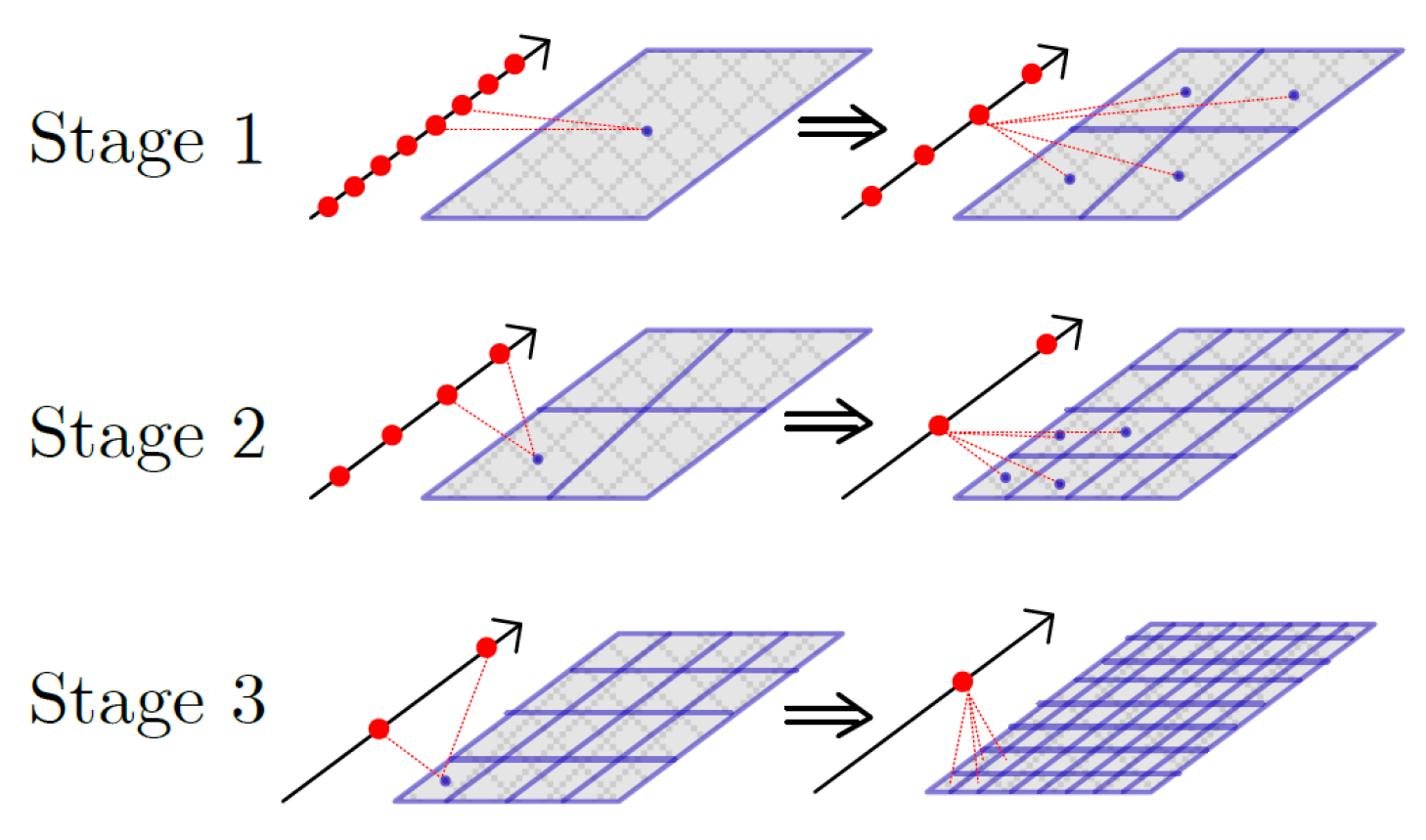
2.2. Subaperture Processing

Following the azimuth de-sampling mentioned above, the pulse repetition frequency (PRF) is also decreased. To avoid aliasing, PRF should be larger than the azimuth bandwidth during each stage of factorization. Subaperture summation is performed in this sense, as shown in a schematic diagram in Figure 1. The left image in Figure 1 shows the data synthesis using the full aperture, while the right image illustrates the subaperture processing. Through the summation of two subapertures, two beams pointing in different directions are obtained. Meanwhile, the beamwidth is halved, and the decreased PRF still satisfies the Nyquist sampling constraint. Subaperture processing is used in many FBP algorithms, such as [19,25].

Suppose that the factorization factor is m and that the beam center of a synthesized aperture on an imaging plane is $\overrightarrow{\mathbf{p}}$. Then, the summation of m subapertures can be written as:

$$s\left(\overrightarrow{\mathbf{x}},\overrightarrow{\mathbf{p}};\tau \right)=\sum _{i=1}^{m}s\left({\overrightarrow{\mathbf{x}}}_i,\overrightarrow{\mathbf{p}};\tau -\Delta {\tau }_i\right)exp\left\{-j2\pi f_0\Delta {\tau }_i\right\},$$

(1)

where $\tau$ is the fast time, $\Delta {\tau }_i$ is the time difference of signal propagating from subaperture $\overrightarrow{\mathbf{x}}$ to $\overrightarrow{\mathbf{p}}$ and from ${\overrightarrow{\mathbf{x}}}_i$ to $\overrightarrow{\mathbf{p}}$,

$$\Delta {\tau }_i=2\frac{\left({\left|\overrightarrow{\mathbf{x}}-\overrightarrow{\mathbf{p}}\right|}_2-{\left|{\overrightarrow{\mathbf{x}}}_i-\overrightarrow{\mathbf{p}}\right|}_2\right)}{c}.$$

(2)

where $f_0$ is the carrier frequency, ${\overrightarrow{\mathbf{x}}}_i$ is the location of the original aperture, $\overrightarrow{\mathbf{x}}$ is the location of the synthesized aperture and $s\left({\overrightarrow{\mathbf{x}}}_i,\overrightarrow{\mathbf{p}}\right)$ is the echo signal at ${\overrightarrow{\mathbf{x}}}_i$.

In this derivation, the summation of subapertures is precise only for the beam center point, for which there is no residual error of slant range. When the scene extends beyond a certain scope, the residual range error will increase, and the summation will deteriorate. To control the maximum error, a partition of the range data according to the multiple beam centers is adopted in Block_FFBP at each stage of subaperture summation. Figure 2 presents an example of the subaperture summation and range data partition in each processing stage. Initially, the number of subapertures is eight. In each stage, the number of subapertures is reduced by a factor of two.

At each stage of subaperture summation in the conventional FBP algorithm, the steering angle and radius are calculated within the local polar coordinate system where the origin is the new aperture. Then, the coordinate of the target and the slant range to the final aperture are determined using subaperture summation. Meanwhile, in the Block_FFBP, the position of the beam center and the corresponding slant range, as well as the differential range are determined for each range block. The slant range of the other points can then be obtained through linear extrapolation using the range and differential range.

The main limitation of Block_FFBP is that the range data are partitioned according to the beam centers; therefore, in the subaperture summation process, the synthesized data in each block can only be obtained through interpolation. If the range dimension partition could be avoided, range data from the identical beam are maintained as a bulk, and the interpolation can be replaced by an FFT. Furthermore, to ensure the interpolation quality of a margin point for a selected interpolation kernel, a fixed backup allowance of the beam data length should be retained. With an increase in the number of factorization stages, the proportion of the interpolation kernel length throughout the entirety of the beam data increases, which indicates that additional memory space is required.

3. Accelerated BP Algorithm

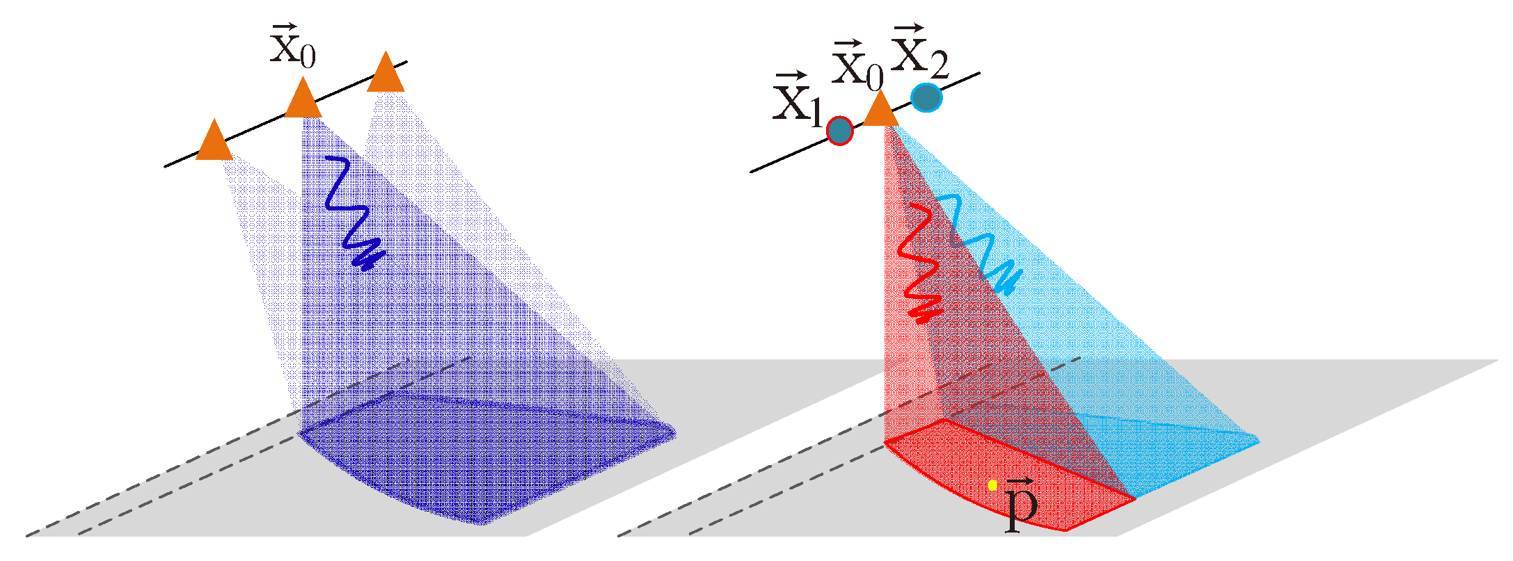
3.1. Fundamental Concept

In this accelerated BP algorithm, a fixed number of pivots, rather than beam centers whose number is variant in each subaperture factorization and summation stage, are applied. Like the general interpolation process, values at sample points are provided, and the interpolated values at specific query points can be obtained using an interpolation method. Pivots are analogous to the sample points. The correspondence relationship of the propagation time delay from these pivots to current and to synthesized subapertures can be constructed. Afterward, the slant range of the other imaging points can be determined using a conventional interpolation method.

Due to oversampling in the angular coordinate system, the slant range calculations are transferred from the polar coordinate system to the Cartesian coordinate system so that the range calculations are simplified. Therefore, this accelerated BP algorithm can be applied in both bistatic and monostatic SAR configurations.

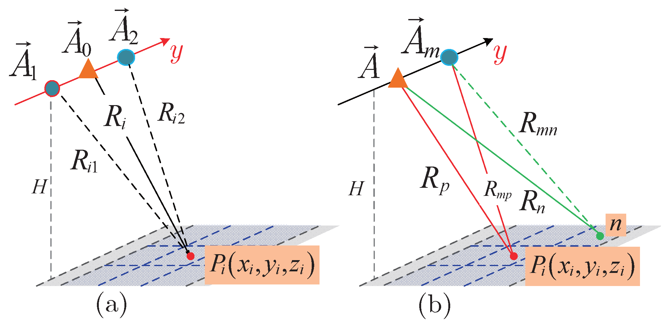
3.2. Monostatic SAR Case

The left image in Figure 3 shows an example of subaperture summation where the factorization factor is two. The platform runs along the y-axis; the x-axis is the range direction; and the z-axis denotes the height dimension. The new subaperture at ${\overrightarrow{\mathbf{A}}}_0\left(x^{\prime },y^{\prime },z^{\prime }\right)$ is the summation of subapertures at ${\overrightarrow{\mathbf{A}}}_1\left(x_1^{\prime },y_1^{\prime },z_1^{\prime }\right)$ and ${\overrightarrow{\mathbf{A}}}_2\left(x_2^{\prime },y_2^{\prime },z_2^{\prime }\right)$. The number of pivots along the range dimension is n, and a pivot can be denoted as ${\overrightarrow{\mathbf{p}}}_i\left(x_i,y_i,z_i\right)$. In this accelerated BP algorithm, the number of pivots is fixed during the focusing process, which is different from Block_FFBP, wherein the number of reference points grows with an increase in the number of factorization stages.

In the left panel of Figure 3, the slant ranges $R_{i1}$, $R_{i2}$ and $R_i$ are the distances between pivot ${\overrightarrow{\mathbf{p}}}_i\left(x_i,y_i,z_i\right)$ and the apertures ${\overrightarrow{\mathbf{A}}}_1\left(x_1^{\prime },y_1^{\prime },z_1^{\prime }\right)$, ${\overrightarrow{\mathbf{A}}}_2\left(x_2^{\prime },y_2^{\prime },z_2^{\prime }\right)$ and ${\overrightarrow{\mathbf{A}}}_0\left(x^{\prime },y^{\prime },z^{\prime }\right)$, respectively. The corresponding time delay can be expressed as:

$${\tau }_{im}=2\frac{{\left|{\overrightarrow{\mathbf{A}}}_m-{\overrightarrow{\mathbf{p}}}_i\right|}_2}{c},\left(m=1,2\right);{\tau }_i=2\frac{{\left|{\overrightarrow{\mathbf{A}}}_0-{\overrightarrow{\mathbf{p}}}_i\right|}_2}{c}$$

(3)

where c is the speed of light. The range-compressed signals belonging to the “old” subapertures ${\overrightarrow{\mathbf{A}}}_1\left(x_1^{\prime },y_1^{\prime },z_1^{\prime }\right)$ and ${\overrightarrow{\mathbf{A}}}_2\left(x_2^{\prime },y_2^{\prime },z_2^{\prime }\right)$ are $s_1\left(\tau \right)$ and $s_2\left(\tau \right)$, respectively. Afterward, according to the subaperture summation stage illustrated in Section 2.2, the “new” synthesized subaperture data $s\left(\tau \right)$ can be written as:

$$s\left({\tau }_i\right)=\sum _{m=1}^2{s}_m\left({\tau }_{im}\right)e^{-j2\pi f_0\left({\tau }_{im}-{\tau }_i\right)},i=1,\dots ,n.$$

(4)

To construct the mapping relationship between the echo delay of the “new” and “old” subapertures, an interpolation function $g_m\left({\tau }_i\right)$ can be used for the delay time pair $\left({\tau }_i,{\tau }_{im}\right)$, which can be expressed as:

$$g_m\left({\tau }_i\right)={\tau }_{im};i=1,2,\dots ,n;m=1,2,$$

(5)

where $g_m\left({\tau }_i\right)$ can be a spline interpolation kernel or a sinc kernel. The subaperture summation can be updated by substituting this interpolation function into Equation (4). The new expression of $s\left(\tau \right)$ is

$$s\left(\tau \right)=\sum _{m=1}^{2}s\left(g_m\left(\tau \right)\right)e^{-j2\pi f_0\left(g_m\left(\tau \right)-\tau \right)}.$$

(6)

Equation (6) is a continuous expression of the subaperture summation process. Hence, partitioning of the range data is favorably avoided, and the complete range data can be processed in bulk. Therefore, the interpolation operation for subaperture data, which is denoted as $s_m\left(·\right)$, can be performed with an FFT to improve the overall efficiency [26].

Equation (3) is a general expression for the monostatic two-way propagation delay, and some simplifications can be made to get a more functional version. If the height of the imaging plane is const $z_0$ and the height of platform is $z_h$, then $z_i=z=z_0;z_m^{\prime }=z^{\prime }=z_h,m=1,2$. Equation (3) becomes:

$$\begin{array}{cc}\hfill {\tau }_{im}& =\frac{2\sqrt{{\left(x_m^{\prime }-x_i\right)}^2+{\left(y_m^{\prime }-y_i\right)}^2+{\left(z_h-z_0\right)}^2}}{c},\hfill \end{array}$$

(7a)

$$\begin{array}{cc}\hfill {\tau }_i& =\frac{2\sqrt{{\left(x^{\prime }-x_i\right)}^2+{\left(y^{\prime }-y_i\right)}^2+{\left(z_h-z_0\right)}^2}}{c},\hfill \end{array}$$

(7b)

In Equation (7b), the range offset $x^{\prime }-x_i$, between “new” subaperture ${\overrightarrow{\mathbf{A}}}_0$ and ${\overrightarrow{\mathbf{p}}}_i$, is:

$$\Delta x_i\left({\tau }_i\right)=-\sqrt{{\left(\frac{{\tau }_i·c}{2}\right)}^2-{\left(y^{\prime }-y_i\right)}^2-{\left(z_h-z_0\right)}^2}.$$

(8)

Substituting Equation (7b) into Equation (7a), a new expression for the time delay can be obtained,

$${\tau }_{im}=\frac{2\sqrt{{\left(x_m^{\prime }-x^{\prime }+\Delta x_i\left({\tau }_i\right)\right)}^2+{\left(y_m^{\prime }-y_i\right)}^2+{\left(z_h-z_0\right)}^2}}{c}.$$

(9)

Furthermore, when the platform runs along a straight trajectory (i.e., $x_m^{\prime }=x^{\prime }$), Equation (9) can be simplified as:

$${\tau }_{im}=\sqrt{{\tau }_i^2+\frac{4}{c^2}\left[{\left({y^{\prime }}_m-y_i\right)}^2-{\left(y^{\prime }-y_i\right)}^2\right]}.$$

(10)

Equation (10) is an analytical expression that can determine the relationship between the two propagation delays of the “new” and “old” subapertures. Let $\Delta ϵ=4\left[{\left({y^{\prime }}_m-y_i\right)}^2-{\left(y^{\prime }-y_i\right)}^2\right]/c^2$; the subaperture summation can be expressed in a continuous form as:

$$s\left(\tau \right)=\sum _{m=1}^{2}s\left(\sqrt{{\tau }^2+\Delta ϵ}\right)e^{-j2\pi f_0\left(\sqrt{{\tau }^2+\Delta ϵ}-\tau \right)}.$$

(11)

Equation (11) represents a case in which the factorization factor is two, and it can be naturally extended to cases with other factorization factors. It is a more simple and practical subaperture summation approach without pivots that facilitates the computational operation. In Equation (10), the locations of “new” and “old” subapertures are only required to be known, and the pivots are no longer required. In this sense, this functional version of Equation (10) is known as range determination. This makes a further simplification of the process. In practice, with the use of fine motion compensation, an equivalent straight line can be obtained, and MoBulk_FFBP can be applied without pivots.

3.3. Bistatic SAR Case

According to the basic principle of the proposed accelerated BP algorithm, this algorithm can also be applied in the bistatic SAR mode. In this section, the accelerated BP algorithm is provided for two bistatic SAR geometries: the one-stationary bistatic SAR mode and the tandem mode. In the former case (including the spaceborne/stationary and the airborne/stationary cases), only the moving platform contributes to the azimuth modulation, whereas the stationary platform introduces a range offset to the range migration trajectories of targets at the same range [14,27]. Therefore, the subaperture summation can be conducted for the moving platform.

Figure 4 shows the subaperture summation for one-stationary bistatic SAR mode where the factorization factor is set to two. The transmitter runs along the y-axis, and the receiver is fixed. $R_{it1}$, $R_{it2}$ and $R_{it}$ are the ranges between ${\overrightarrow{\mathbf{p}}}_i\left(x_i,y_i,z_i\right)$ and the transmitter subapertures ${\overrightarrow{\mathbf{A}}}_1\left(x_1^{\prime },y_1^{\prime },z_1^{\prime }\right)$, ${\overrightarrow{\mathbf{A}}}_2\left(x_2^{\prime },y_2^{\prime },z_2^{\prime }\right)$, ${\overrightarrow{\mathbf{A}}}_0\left(x^{\prime },y^{\prime },z^{\prime }\right)$, respectively; while, $R_{ir}$ is the range between the receiver and ${\overrightarrow{\mathbf{p}}}_i$. Thus, the echo delay for each subaperture can be written as:

$$\begin{array}{cc}\hfill {\tau }_{im}& =\frac{R_{itm}+R_{ir}}{c},(m=1,2),\hfill \\ \hfill {\tau }_i& =\frac{R_{it}+R_{ir}}{c}\hfill \end{array}$$

(12)

The data of “new” subaperture ${\overrightarrow{\mathbf{A}}}_0$ can also be obtained using Equation (6). For a given range line in the focus plane parallel to the transmitter trajectory, the range to the receiver is different for each grid point. Therefore, it is difficult to obtain an analytical expression for the subaperture summation without deriving a relationship for the location of the pivots.

However, in the azimuth-invariant bistatic SAR mode, this situation may be different [11,28]. The delay times for the “old” and “new” subapertures are:

$$\begin{array}{cc}\hfill {\tau }_{im}& =\frac{R_{itm}+R_{irm}}{c},m=1,2\hfill \\ \hfill {\tau }_i& =\frac{R_{it}+R_{ir}}{c}\hfill \end{array}$$

(13)

For this mode, let the “new” subapertures of a transmitter and receiver be ${\overrightarrow{\mathbf{A}}}_0\left(x_1,y_1,z_1\right)$ and ${\overrightarrow{\mathbf{A}}}_0\left(x_2,y_2,z_2\right)$, respectively. Let $R_i={\tau }_i·c$,

$$\begin{array}{cc}\hfill R_{it}& =\sqrt{{\left(x_1-x_i\right)}^2+{\left(y_1-y_i\right)}^2+{\left(z_1-z_i\right)}^2}\hfill \\ \hfill R_{ir}& =\sqrt{{\left(x_2-x_i\right)}^2+{\left(y_2-y_i\right)}^2+{\left(z_2-z_i\right)}^2}\hfill \end{array}$$

(14)

For convenience, let $c_1={\left(y_1-y_i\right)}^2+{\left(z_1-z_i\right)}^2$, $c_2={\left(y_2-y_i\right)}^2+{\left(z_2-z_i\right)}^2$ and $c_3=x_1-x_2$; thus, $x_i\left({\tau }_i\right)$ can be solved as

$$x_i\left({\tau }_i\right)=\frac{-b+\sqrt{b^2-a·d}}{2a}$$

(15)

where:

$$\begin{array}{cc}\hfill a& =c_3^2-{\left(c·{\tau }_i\right)}^2,\hfill \\ \hfill b& =c_3\left[c_1-c_2+a\right],\hfill \\ \hfill d& =c_1^2+c_2^2+a^2-2c_1\left(c_2-a\right)-2c_2\left[c_3^2+{\left(c·{\tau }_i\right)}^2\right].\hfill \end{array}$$

(16)

Therefore, ${\tau }_{im}\left({\tau }_i\right)$ can be obtained by substituting (15) into ${\tau }_{im}$ in Equation (13). Similar to Equation (11), the subaperture summation can also be expressed in a continuous form:

$$s\left(\tau \right)=\sum _{m=1}^{2}s\left({\tau }_m\left(\tau \right)\right)e^{-j2\pi f_0\left({\tau }_m\left(\tau \right)-\tau \right)}$$

(17)

3.4. Summary of the Algorithm

Figure 5 presents the flowchart of proposed algorithm. The green and cyan blocks represent processing with and without pivots, respectively. Range compression is conducted in the first stage. The number of factorization stages and the factorization factor in each stage are set. For the general case, pivots are required. According to Equation (5), an interpolation function is used to calculate the delay time of the “new” subapertures, which corresponds to the propagation time delay reconstruction in Figure 5. Specifically, when the platform runs along a straight track, pivots are not required, and in the factorization stage, delay time is determined according to Equation (10). After the propagation time delay relationship is established, range data interpolation is performed using an FFT followed by the subaperture summation. When the factorization is done, a conventional BP algorithm is applied to focus the new synthetic data, and a final focused image is obtained.

4. Performance Analysis

4.1. Error Analysis

This section provides the phase error caused by an incorrect slant range when the back-projected data are accumulated during a subaperture summation. Since the proposed algorithm is derived from Block_FFBP and extended to the bistatic SAR case, the error analysis will be conducted through a comparison with Block_FFBP using a numerical method. Moreover, as Block_FFBP was developed for the monostatic SAR case, the error analysis is mainly performed for this case.

In Block_FFBP, the slant range error between the “old” and ”new” subapertures causes a phase error, which can affect the focusing. For a certain imaging block, like the right panel in Figure 3, only the delay time of the beam center point ${\overrightarrow{\mathbf{p}}}_i$ is correct during the subaperture summation. Assume that ${\overrightarrow{\mathbf{A}}}_m$ is the “old” subaperture and $\overrightarrow{\mathbf{A}}$ is the “new” one. Point $\overrightarrow{\mathbf{n}}$ is one grid point in the block. The slant ranges from ${\overrightarrow{\mathbf{p}}}_i$ to ${\overrightarrow{\mathbf{A}}}_m$ and to $\overrightarrow{\mathbf{A}}$ are $R_{mp}$ and $R_p$, respectively. Likewise, for point $\overrightarrow{\mathbf{n}}$, the slant ranges are $R_{mn}$ and $R_n$, respectively. In Block_FFBP, the slant range of “new” aperture $\overrightarrow{\mathbf{A}}$ should be mapped to the “old” aperture to perform the subaperture summation. For any point $\overrightarrow{\mathbf{n}}$, the obtained range is $R_{mn}^{\prime }=R_n+R_{mp}-R_p$, and the two-way delay time error caused by this operation is:

$$\Delta {\tau }_{error}=\frac{2}{c}·\left(R_{mn}-R_{mn}^{\prime }\right)=\frac{2}{c}·\left(R_{mn}-R_n-\left(R_{mp}-R_p\right)\right).$$

(18)

Thus, the residual phase error can be written as:

$$\Delta {\varphi }_1=2\pi f_0·\Delta {\tau }_{error}.$$

(19)

In MoBulk_FFBP, the beam center point $\overrightarrow{\mathbf{p}}$ in the right panel of Figure 3 can also be taken as a pivot. When the subaperture summation is performed using Equation (6), the residual phase error of point $\overrightarrow{\mathbf{n}}$ can be written as:

$$\Delta {\varphi }_2=2\pi f_0·\left[g_m\left(\frac{2R_n}{c}\right)-\frac{2R_{mn}}{c}\right],$$

(20)

where $g_m(·)$ is the interpolation kernel defined by Equation (5). Moreover, when the platform runs along a straight trajectory, pivots are not required, and points that have the same azimuth coordinates as $\overrightarrow{\mathbf{p}}$ have no phase error. The residual phase error can be expressed as:

$$\Delta {\varphi }_3=2\pi f_0·\left[\sqrt{{\left(\frac{2R_n}{c}\right)}^2+\Delta ϵ}-\frac{2R_{mn}}{c}\right].$$

(21)

Here, a numerical simulation is conducted to intuitively compare these phase errors. An airborne geometry with a straight trajectory, a platform height of 8 km, an off-nadir angle of ${40}^{°}$ and a carrier frequency of 9.6 GHz are investigated. The offset range between the “new” and “old” subapertures $\left|A{A}_m\right|$ varies from 1 m–1000 m, and the squint angle varies from $0^{°}$–${24}^{°}$. For a certain offset and squint angle, the scene size is set according to the principle that the maximum residual phase error of an imaging point in the scene is $\pi /8$. In each such scene, a 200 × 200 point array is set. Through statistics, the maximum $\Delta {\varphi }_2$ or $\Delta {\varphi }_3$ of these points is obtained. To compare these with $\Delta {\varphi }_1$, the maximum residual phase error is normalized by $\pi /8$. The final result is shown in Figure 6.

The top yellow plane in Figure 6 is the residual phase error of Block_FFBP, which is normalized by $\pi /8$. A larger offset range between the “new” and “old” subapertures and a smaller residual phase error for the proposed MoBulk_FFBP can be observed. Moreover, under this simulation configuration, the residual phase error decreases with the squint angle, which varies from $0^{°}$ to ${18}^{°}$. Although the phase error increases from ${18}^{°}$–${25}^{°}$ in this experiment, the overall phase error is lower than that of Block_FFBP, which could validate the accuracy of the proposed algorithm.

4.2. Parallelization

As is shown in Figure 5, the factorization is operated sequentially. However, the range data are processed as a bulk set, and the upsampling of this is performed using an FFT in each stage of subaperture summation. In this sense, each stage of the factorization can be executed in parallel. Moreover, after factorization, the conventional BP algorithm can also be executed in parallel, such as with a GPU [29,30] or a multi-thread technical CPU. This will further accelerate the proposed algorithm.

4.3. Computational Complexity

A detailed theoretical derivation of the computational complexity of the proposed algorithm is provided here. Suppose that the aperture length is L and the data size is $N\left(Az\right)\times M\left(Rg\right)$. “Az” and “Rg” denote the azimuth and range dimension, respectively. In the processing, a factorization of L into K integer factors, corresponding to K processing stages, is established. The reduction in the number of apertures is defined as $l_i,(i=1,2,\dots ,K)$, and L can be expressed as:

$$L=l_1\times l_2\times l_3\times \cdots \times l_K.$$

(22)

For simplicity, a common factorization throughout all of the stages is used ($l_i=n$ for all i); then, $L=n^K$, and $K={log}_{n}N$. The number of pivots is set to Q and is fixed at each stage. The aperture length is equal to the azimuth data length such that $L=N$.

In the first stage, the original aperture is split into $N/n$ subapertures, each of which has a length n. To construct the mapping relationship between the echo delays of the “new” and “old” subapertures, an efficient cubic spline interpolation scheme [31] is used. As demonstrated in [31], this spline interpolation is very efficient: $O\left(Q\right)$ is used to generate the spline, and $O(logQ)$ is used to evaluate the spline at a single point, where Q is the number of input data points. Thus, the interpolation computational burden is $\frac{N}{n}\times n\left(Q+MlogQ\right)$. Next, the interpolation of range data is implemented using upsampling with an FFT, and the overall computational complexity for the FFT and inverse FFT is $\frac{N}{n}\times n\left(MlogM+\alpha Mlog\alpha M\right)$, where $\alpha$ is the upsampling rate. At this stage, the number of beams is n, and the computational burden required to form the beams is:

$$\frac{N}{n}\left(subapertures\right)\times n\left(subaperturepoints\right)\times \left(nM\right)\left(beamssamples\right).$$

(23)

Equation (23) can be written as $nMN$ for simplicity. Based on the first factorization stage, the second processing stage forms $N/n^2$ new beams. Because of the common number of pivots and the unchanged number of range data, the operations for interpolation and upsampling are the same as those in the first stage. The number of operations required to form new beams becomes $\frac{N}{n^2}\times n\times \left(n^{2}M\right)=nMN$. Therefore, each processing stage has the same number of operations, and the total computational complexity can be written as:

$$\left[N\left(Q+MlogQ+MlogM+\alpha Mlog\alpha M\right)+nMN\right]\times {log}_{n}N.$$

(24)

4.4. Pivot Selection Issue

During the factorization and subaperture summation process, the accuracy of signal propagation time between the “new” and “old” subapertures could affect the final image quality. In Block_FFBP, the slant range computation error changes across the data block. In the proposed algorithm, the accuracy of slant range can be ensured by the interpolation, which is described in Equation (5). To evaluate the influence of the chosen number of pivots, slant range computation errors between “new” and “old” subapertures are calculated in the condition of different swaths and different number of pivots. Assume that the platform height is 8 km, the look angle is ${40}^{°}$ and the subaperture offset is 400 m. The interpolation scheme is a spline function.

In this simulation, the number of pivots changes from 4–64, and pivots are distributed along the range dimension at the same intervals. First, 3000 points are located along the range direction with different range extensions. The average slant computation error is shown in Figure 7a. Second, 3000 points are located along the azimuth dimension with different azimuth extensions. The average slant computation error is shown in Figure 7b.

It can be seen that due to the high accuracy of spline interpolation, the slant range computation is very accurate. The influence of different chosen numbers of pivots is ignorable and varies slightly. In this sense, the choice of pivots is flexible. Please note that in the experiment, the smallest number of pivots is four; this is because the spline interpolation method requires at least four sampling points.

5. Simulation and Real Data Results

In this section, the accuracy and efficiency of the proposed algorithm are validated using point target simulation and real data. The time cost for each stage of the factorization is also taken into consideration. Due to the parallelizability of the processing scheme, a horizontal comparison between different parallel processing strategies is given. For the azimuth-invariant bistatic SAR case, synthesized SAR data are utilized to confirm the performance of the algorithm. Meanwhile, for the spaceborne/stationary bistatic SAR configuration, real data acquired on 31 January, 2015, using TerraSAR-X as an illuminator in the staring spotlight mode, are used for validation.

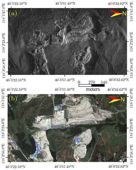
5.1. Monostatic SAR Case

Airborne monostatic SAR data in spotlight mode with a straight trajectory are investigated here. The simulation parameters are given in

Table 1. Simulation parameters of the monostatic SAR case. PRF, pulse repetition frequency.

Parameter	Values
Carrier frequency (GHz)	9.6
Bandwidth (MHz)	400
PRF (Hz)	160
Platform height (km)	10
Look angle (°)	4
Velocity (m/s)	120
Azimuth steering angle (°)	±1.62

. In this scene, a $5\times 5$ point array is established, and the spacing between each point is 1000 m. The simulated echo signal is focused using the proposed MoBulk_FFBP (both with and without pivots), FFBP and Block_FFBP. All algorithms have four processing stages with a common factorization factor of four for each stage. In MoBulk_FFBP with pivots, the number of pivots is 32, and the interpolation kernel used in this experiment is a spline kernel. In the simulation, the focusing results of the two versions of MoBulk_FFBP are almost identical. The results are shown in Figure 8.

Figure 8c indicates that the focusing quality of MoBulk_FFBP is adequate. A close look at the upper right target is shown intuitively in Figure 9. By examining the acquired range and azimuth profiles through the peak of the focused target, the impulse-response width (IRW), peak sidelobe ratio (PSLR), integrated sidelobe ratio (ISLR) and signal-to-noise (SNR) are evaluated and summarized in

Table 2. Accuracy measurements. IRW, impulse-response width; PSLR, peak sidelobe ratio; ISLR, integrated sidelobe ratio; Az, azimuth; Rg, range.

	IRW (dB)	PSLR (dB)	ISLR (dB)	SNR (dB)
FFBP	(Rg)0.53/(Az)0.28	(Rg)-12.35/(Az)-13.04	(Rg)-9.82/(Az)-9.7	52.61
Block_FFBP	(Rg)0.53/(Az)0.28	(Rg)-12.36/(Az)-13.11	(Rg)-6.9254/(Az)-10.1	50.25
MoBulk_FFBP	(Rg)0.53/(Az)0.28	(Rg)-12.33/(Az)-12.99	(Rg)-10.93/(Az)-9.58	53.39

. According to the system parameters, the theoretical IRWs in the range and azimuth directions are 0.525 and 0.276 m, respectively. The measured range and azimuth IRWs agree well with the theoretical values. The deviations of PSLRs in each profile are within 0.2 dB of the theoretical values of −13.26 dB. Meanwhile, in Figure 9b, the focusing quality in the azimuth direction is decent, while the amplitude of third sidelobe in the range direction indicated by the red arrow is higher than the standard level, which causes the ISLR to deviate from the theoretical value, and the SNR decreases. This ringing effect of pulse response in the range direction is introduced by the data partition. As explained above, the upsampling operation can only be performed through interpolation rather than with an FFT due to the effects of data partitioning. The ringing effect of the interpolation can become increasingly stronger after each stage of the factorization. In the proposed algorithm, range data are processed in bulk rather than in blocks; according to the measured SNRs, it can be seen that the ‘focusing depth’ of MoBulk_FFBP is higher.

To compare the efficiency, the raw data of these points are focused by Block_FFBP and MoBulk_FFBP independently with different factorization stages. Since it has been demonstrated in [19] that Block_FFBP is much more computationally efficient than FFBP, thus the comparison of computation complexity with FFBP is not conducted here. The programs are executed in a single-threaded environment, and the factorization factor is four in each processing stage. The hardware configuration is listed in

Table 3. Hardware configuration for simulation.

Items	Values
CPU	Xeon E5620
Clock speed	2.4 GHz
Memory	192 GB

. Let K be the number of factorization stages. In Figure 10a, the smaller processing time cost indicates that the processing efficiency of MoBulk_FFBP is generally higher than that of Block_FFBP. This is because the required memory of Block_FFBP at each stage is unstable, which increases the time cost for the factorization and reduces the overall efficiency. The trend shown in Figure 10a indicates that the time cost diminishes as K rises. However, in this experiment, the required processing time increases when K is larger than five. The entire processing scheme incorporates the factorization and BP focusing of the accumulated data. Figure 10b shows the time costs for these two steps for MoBulk_FFBP and Block_FFBP, respectively. First, the time cost for the factorization stage rises as K rises; on the contrary, the time cost decreases for increasing K values for the following residual BP step. Moreover, the time cost for the factorization of MoBulk_FFBP is larger than that of Block_FFBP when K is less than five. This is due to the fact that the interpolation kernel is short and the interpolation computation speed is low for the subaperture summation. When K becomes larger, the time cost for the factorization of Block_FFBP increases dramatically. Then, the time cost for the subsequent BP operation of MoBulk_FFBP is much less than that of Block_FFBP, which benefits from upsampling with an FFT instead of interpolation.

After the point target simulation, the raw data of synthesized distributed scene containing land and water are generated. Figure 11a–d shows the focusing results, which are processed using BP, MoBulk_FFBP, FFBP and Block_FFBP, respectively. In the red rectangle in each figure, the focusing quality of Block_FFBP is not as good as the others due to the residual phase error induced by the changing range error. The water area in the green rectangle is used for SNR comparison. From Figure 11a–d, the measured SNR is 22.83 dB, 22.78 dB, 22.46 dB and 22.61 dB. although the SNR of each result are similar, the SNR of MoBulk_FFBP is a little better. However, the focusing performance can be validated by the area in the red rectangle.

Here, the MoBulk_FFBP will be validated using real airborne data, which were acquired in a spotlight SAR experiment taken in Zunhua, China, on June 2016. The radar data were acquired with an airborne wideband SAR operating at a 1200 MHz bandwidth. The carrier frequency was 9.6 GHz, and the PRF was 2000 Hz. The flight altitude was approximately 7500 m, and the track was measured using both a GPS and an INS. The local incidence angle of the scene center is ${66}^{°}$. To apply MoBulk_FFBP, a procedure is designed to focus the data. First, the equivalent velocity is computed using the Doppler centroid frequency, which is calculated using the azimuth cross correlation. Then, motion compensation [32,33] is performed using the platform velocity in the east, north and up directions provided by the INS. After motion compensation, the equivalent velocity is corrected and updated. With the location information provided by the GPS and the obtained equivalent velocity, a straight flight track is fitted. The focusing plane is set equal with the average scene height. Then, the MoBulk_FFBP with or without pivots can be applied to focus the data. The focused monostatic spotlight SAR image is shown in Figure 12. The result indicates that MoBulk_FFBP exhibits a satisfactory processing performance. According to the aforementioned subaperture summation principle, the MoBulk_FFBP was established with an aperture block size of 256, i.e., the 24,576 aperture positions in the echo data were divided into 96 blocks. Four aperture positions are summed in each processing stage until the entire block is processed during the four stages. In this sense, all of the processing stages correspond to an aperture factorization according to 24,576 = $4^4\times 96$. The subaperture summation is conducted using Equation (8), and the range data upsampling operation is performed in bulk with an FFT.

5.2. Bistatic SAR Case

To demonstrate the focusing ability of the proposed algorithm for the bistatic SAR case, an azimuth-invariant bistatic spotlight configuration is initially investigated. The transmitter and receiver run along straight trajectories that are separated by 5 m. The system parameters are the same as the point target simulation in the monostatic SAR case. The focused master and slave SAR images are shown in Figure 11b,e, and the result indicates that BiBulk_FFBP can also perform well. Due to the relatively short baseline, the results are very similar, but they demonstrate a slight difference in the marked zone. The factorization factor of BiBulk_FFBP is four, which means that four aperture positions are summed in each processing stage until the entire block is processed, thereby requiring four stages.

Spaceborne/stationary bistatic SAR also use a bistatic SAR configuration that is easily implemented using orbital sensors as coherent transmitters of opportunity with fixed-location receivers. Here, the fast back projection for focusing the one-stationary bistatic SAR data proposed in [25] is used for accuracy comparison. It can handle the synchronization problem and focus the data more efficiently than the BP algorithm, which makes it very appropriate for spaceborne/stationary bistatic SAR processing. A point target simulation based on a spaceborne/stationary bistatic configuration is conducted, and the parameters are given in

Table 4. Spaceborne/stationary bistatic SAR simulation parameters.

Parameter	Values
Carrier frequency (GHz)	9.6
Bandwidth (MHz)	150
Sampling rate (MHz)	180
Pulse repetition frequency (Hz)	8000
Synthetic aperture time (s)	1.27
Transmitter center position (km)	(0, 400, 692.8203)
Synchronization channel position (m)	(0, 0, 533)
Echo channel position (m)	(0, 0, 533)
Target for evaluation (m)	(−320, −9216, 0)

.

The results processed by the FBP in [25] and the proposed BiBulk_FFBP are shown in Figure 13. To evaluate the IRW, PSLR and ISLR, the contours of the point at left-up corner are enlarged and shown in Figure 14.

In Figure 14, it can be intuitively found that the focusing quality of BiBulk_FFBP is better that of the FBP in [25]. This is because the series of sub-images is focused at fixed grids, and the nearest interpolation method is used in the sub-images fusion process. Therefore, the imaging quality of the final image is nonuniform. The measured SNR of Figure 13a,b is 58.83 dB and 58.79 dB. From the two-dimensional profiles, it can be seen that two versions of fast BP algorithm have similar performance. However, from the perspective of computational complexity, BiBulk_FFBP is more computational efficient. Equation (24) can be approximated as $n{N}^2{log}_{n}N$. Comparing with the computational complexity of FBP in [25], $N^{2.5}$, the computational cost of BiBulk_FFBP is lower.

On 31 January 2015, a spaceborne/stationary bistatic SAR (SS-BiSAR) experiment with the transmitter, TerraSAR-X, operating in ST mode was conducted by the Institute of Electronics, Chinese Academy of Sciences (IECAS). More details about the system configuration and the preprocessing of the raw data are provided in [34]. In this experiment, the direct signal was used as the matched filter to perform the range compression. With this method, the time synchronization error, phase synchronization error and tropospheric delay error are eliminated. Ignoring the two-dimensional envelop function, the compressed and synchronized signal in the range frequency domain is:

$$S_{com}\left(\tau ,f;\tilde{\mathbf{r}}\right)=e^{-j2\pi f\frac{R_{TR}\left(\tau ;\tilde{\mathbf{r}}\right)-R_D\left(\tau \right)}{c}}$$

(25)

where $\tau$ is the azimuth time, f is the range frequency, $R_D\left(\tau \right)$ is the direct signal path and $R_{TR}\left(\tau ;\tilde{\mathbf{r}}\right)$ denotes the signal propagation range for a target located at $\tilde{\mathbf{r}}$. According to the information given in the TerraSAR-X product file, an XML file, the direct pulse phase history compensation can be performed in the SS-BiSAR coordinate system, after which the range-compressed signal becomes:

$$S_{com}\left(\tau ,f;\tilde{\mathbf{r}}\right)=e^{-j2\pi f\frac{R_T\left(\tau ;\tilde{\mathbf{r}}\right)+R_R\left(\tilde{\mathbf{r}}\right)}{c}}$$

(26)

After performing the direct pulse phase history compensation and an inverse Fourier transformation, the range-compressed signal can be focused using the BiBulk_FFBP. In this experiment, the factorization factor is four, and the four subapertures in each of the four stages are summed into a new one. The focused result is shown in Figure 15. The magnified Areas A and B are also shown in the right panel. Area A is located in the near range of the receiver, from which a high SNR is consequently obtained. Because of the large incidence angle of the receiver, the tree canopies are clearly identified, and the track of an athletic field is easily recognized. Area B has some buildings that were still in construction at the time of data acquisition, and two tower slewing cranes are clearly focused. These details validate the focusing ability of the proposed BiBulk_FFBP.

As previously discussed, each stage of factorization can be executed in parallel, which further accelerates the processing scheme. To show the acceleration with a multi-thread operation, the factorization and subsequent BP are executed in a single-threaded (ST) and a multi-threaded (MT) environment, respectively. The results are shown in Figure 16. The hardware configuration is shown in Table 3. The computation time of the raw radar data containing 1536 MSampleson an image grid of 144 MPointsis 203.6 min, 306 min and 400.405 min for MT-MT, ST-MT and MT-ST processing pairs, respectively. Therefore, the parallelization of the processing scheme provides a large increase in computational speed compared to the conventional BP algorithm. Moreover, when the program is executed within a GPU platform, the computation speed is even faster.

6. Conclusions

In this paper, an accelerated BP algorithm is proposed to focus monostatic and bistatic SAR data. In this algorithm, the range data are processed in bulk rather than through block partitions. This unified range data processing scheme improves the computational efficiency and simplifies the procedure. A fixed number of pivots rather than beam centers is applied to construct the relationship of the propagation time delay between the “new” and “old” subapertures. Moreover, when the trajectory is a straight line, the pivots are not required, and the analytical expression of the subaperture summation can be derived for the monostatic and azimuth-invariant bistatic SAR case. Error analysis shows that the accuracy of the proposed algorithm is verifiable. Since the algorithm is an improved version of Block_FFBP, it satisfies numerical performance standards and retains the processing ability of Block_FFBP. Moreover, it can also focus the bistatic SAR data acquired from the tandem mode and the one-stationary bistatic SAR mode. Simulation data and real radar data validate the performance of the algorithm.

References

1. Franceschetti, G.; Lanari, R. Synthetic Aperture Radar Processing; CRC Press: Boca Raton, FL, USA, 1999; pp. 32–58. [Google Scholar]
2. Cumming, I.G.; Bennett, J. Digital processing of SeaSAT SAR data. In Proceedings of the IEEE International Conference on ICASSP ’79 Acoustics, Speech, and Signal Processing, Washington, DC, USA, 2–4 April 1979; pp. 710–718. [Google Scholar]
3. Raney, R.K.; Runge, H.; Bamler, R.; Cumming, I.G.; Wong, F.H. Precision SAR processing using chirp scaling. IEEE Trans. Geosci. Remote Sens. 1994, 32, 786–799. [Google Scholar] [CrossRef]
4. Carrara, W.G.; Majewski, R.M.; Goodman, R.S. Spotlight Synthetic Aperture Radar: Signal Processing Algorithms; Artech House: Norwood, MA, USA, 1995. [Google Scholar]
5. Bamler, R.; Eineder, M. ScanSAR processing using standard high precision SAR algorithms. IEEE Trans. Geosci. Remote Sens. 1996, 34, 212–218. [Google Scholar] [CrossRef]
6. Mittermayer, J.; Moreira, A. Spotlight SAR processing using the extended chirp scaling algorithm. In Proceedings of the 1997 IEEE International IGARSS’97, Remote Sensing—A Scientific Vision for Sustainable Development, Singapore, 3–8 August 1997; pp. 2021–2023. [Google Scholar]
7. Loffeld, O.; Nies, H.; Peters, V.; Knedlik, S. Models and useful relations for bistatic SAR processing. IEEE Trans. Geosci. Remote Sens. 2004, 42, 2031–2038. [Google Scholar] [CrossRef]
8. Natroshvili, K.; Loffeld, O.; Nies, H.; Ortiz, A.M.; Knedlik, S. Focusing of general bistatic SAR configuration data with 2-D inverse scaled FFT. IEEE Trans. Geosci. Remote Sens. 2006, 44, 2718–2727. [Google Scholar] [CrossRef]
9. Wang, R.; Loffeld, O.; Nies, H.; Knedlik, S.; Ender, J.H.G. Chirp-scaling algorithm for bistatic SAR data in the constant-offset configuration. IEEE Trans. Geosci. Remote Sens. 2009, 47, 952–964. [Google Scholar] [CrossRef]
10. Neo, Y.L.; Wong, F.H.; Cumming, I.G. Processing of azimuth-invariant bistatic SAR data using the range Doppler algorithm. IEEE Trans. Geosci. Remote Sens. 2008, 46, 14–21. [Google Scholar] [CrossRef]
11. Bamler, R.; Meyer, F.; Liebhart, W. Processing of bistatic SAR data from quasi-stationary configurations. IEEE Trans. Geosci. Remote Sens. 2007, 45, 3350–3358. [Google Scholar] [CrossRef]
12. Wong, F.H.; Cumming, I.G.; Neo, Y.L. Focusing bistatic SAR data using the nonlinear chirp scaling algorithm. IEEE Trans. Geosci. Remote Sens. 2008, 46, 2493–2505. [Google Scholar] [CrossRef]
13. Qiu, X.; Hu, D.; Ding, C. An improved NLCS algorithm with capability analysis for one-stationary BiSAR. IEEE Trans. Geosci. Remote Sens. 2008, 46, 3179–3186. [Google Scholar] [CrossRef]
14. Zeng, T.; Hu, C.; Wu, L.; Liu, L.; Tian, W.; Zhu, M.; Long, T. Extended NLCS algorithm of BiSAR systems with a squinted transmitter and a fixed receiver: Theory and experimental confirmation. IEEE Trans. Geosci. Remote Sens. 2013, 51, 5019–5030. [Google Scholar] [CrossRef]
15. Wang, R.; Loffeld, O.; Nies, H.; Ender, J.H.G. Focusing spaceborne/airborne hybrid bistatic SAR data using wavenumber-domain algorithm. IEEE Trans. Geosci. Remote Sens. 2009, 47, 2275–2283. [Google Scholar] [CrossRef]
16. Tang, J.; Deng, Y.; Wang, R.; Zhao, S.; Li, N.; Wang, W. A weighted backprojection algorithm for azimuth multichannel SAR imaging. IEEE Geosci. Remote Sens. Lett. 2016, 13, 1265–1269. [Google Scholar] [CrossRef]
17. Behner, F.; Reuter, S.; Nies, H.; Loffeld, O. Synchronization and processing in the HITCHHIKER bistatic SAR experiment. IEEE J. Sel. Top. Appl. Earth Obs. Remote Sens. 2016, 9, 1028–1035. [Google Scholar] [CrossRef]
18. Yegulalp, A.F. Fast backprojection algorithm for synthetic aperture radar. In Proceedings of the The Record of the 1999 IEEE Radar Conference, Waltham, MA, USA, 22 April 1999; pp. 60–65. [Google Scholar]
19. Ulander, L.M.H.; Hellsten, H.; Stenstrom, G. Synthetic-aperture radar processing using fast factorized back-projection. IEEE Trans. Geosci. Remote Sens. 2003, 39, 760–776. [Google Scholar] [CrossRef]
20. Rodriguez-Cassola, M.; Baumgartner, S.V.; Krieger, G.; Moreira, A. Bistatic TerraSAR-X/F-SAR spaceborne/airborne SAR experiment: Description, data processing, and results. IEEE Trans. Geosci. Remote Sens. 2010, 48, 781–794. [Google Scholar] [CrossRef] [Green Version]
21. Duque, S.; Lopez-Dekker, P.; Mallorqui, J.J. Single-pass bistatic SAR interferometry using fixed-receiver configurations: Theory and experimental validation. IEEE Trans. Geosci. Remote Sens. 2010, 48, 2740–2749. [Google Scholar] [CrossRef] [Green Version]
22. Walterscheid, I.; Espeter, T.; Brenner, A.R.; Klare, J.; Ender, J.H.G.; Nies, H.; Wang, R.; Loffeld, O. Bistatic SAR experiments with PAMIR and TerraSAR-x;setup, processing, and image results. IEEE Trans. Geosci. Remote Sens. 2010, 48, 3268–3279. [Google Scholar] [CrossRef]
23. Vu, V.T.; Sjogren, T.K.; Pettersson, M.I. Fast time-domain algorithms for UWB bistatic SAR processing. IEEE Trans. Aerosp. Electron. Syst. 2013, 49, 1982–1994. [Google Scholar] [CrossRef]
24. Rodriguez-Cassola, M.; Prats, P.; Krieger, G.; Moreira, A. Efficient time-domain image formation with precise topography accommodation for general bistatic SAR configurations. IEEE Trans. Aerosp. Electron. Syst. 2011, 47, 2949–2966. [Google Scholar] [CrossRef] [Green Version]
25. Shao, Y.; Wang, R.; Deng, Y.; Liu, Y.; Chen, R.; Liu, G.; Loffeld, O. Fast backprojection algorithm for bistatic SAR imaging. IEEE Geosci. Remote Sens. Lett. 2013, 10, 1080–1084. [Google Scholar] [CrossRef]
26. Cumming, I.G.; Wong, F.H. Digital Processing of Synthetic Aperture Radar Data: Algorithms and Implementation; Artech House: Norwood, MA, USA, 2005; pp. 32–58. [Google Scholar]
27. Wang, R.; Loffeld, O.; Neo, Y.L.; Nies, H.; Walterscheid, I.; Espeter, T.; Klare, J.; Ender, J.H.G. Focusing bistatic SAR data in airborne/stationary configuration. IEEE Trans. Geosci. Remote Sens. 2010, 48, 452–465. [Google Scholar] [CrossRef]
28. Walterscheid, I.; Ender, J.H.G.; Brenner, A.R.; Loffeld, O. Bistatic SAR processing and experiments. IEEE Trans. Geosci. Remote Sens. 2010, 44, 2710–2717. [Google Scholar] [CrossRef]
29. Shi, J.; Long, X.; Zhang, X. Streaming BP for non-linear motion compensation SAR imaging based on GPU. IEEE J. Sel. Top. Appl. Earth Obs. Remote Sens. 2013, 6, 2035–2050. [Google Scholar] [CrossRef]
30. Di Bisceglie, M.; Di Santo, M.; Galdi, C.; Lanari, R.; Ranaldo, N. Synthetic aperture radar processing with GPGPU. IEEE Signal. Proc. Mag. 2010, 27, 69–78. [Google Scholar] [CrossRef]
31. Kluge, T. Pricing Swing Options and Other Electricity Derivatives. Ph.D. Dissertation, St Hugh’s College, University of Oxford, Oxford, UK, 2006. Available online: http://kluge.in-chemnitz.de/docs/phd/ (accessed on 11 July 2006).
32. Nies, H.; Loffeld, O.; Na, K.; Natroshvili, F. Analysis and focusing of bistatic airborne SAR data. IEEE Trans. Geosci. Remote Sens. 2007, 45, 3342–3349. [Google Scholar] [CrossRef]
33. Mao, X.; Zhu, D.; Zhu, Z. Autofocus correction of ape and residual rcm in spotlight SAR polar format imagery. IEEE Trans. Aerosp. Electron. Syst. 2013, 49, 2693–2706. [Google Scholar] [CrossRef]
34. Zhang, H.; Deng, Y.; Wang, R.; Li, N.; Zhao, S.; Hong, F.; Wu, L.; Loffeld, O. Spaceborne/stationary bistatic SAR imaging with TerraSAR-X as an illuminator in staring-spotlight modeAnalysis and focusing of bistatic airborne SAR data. IEEE Trans. Geosci. Remote Sens. 2007, 54, 5203–5214. [Google Scholar] [CrossRef]
Figure 1. Subaperture summation progress. In the left panel, ‘triangle’ denotes the location where the platform transmits the signal. In the right panel, x 1 and x 2 denote two subapertures and x 0 denote the new synthesized aperture.
Remotesensing 10 00140 g001
Figure 2. Schematic illustration of the FFBP with eight apertures and three factorization stages. In each processing stage, a common factorization factor of two is used. Narrower “new” beams are formed based on wider “old” beams formed in the previous stage. In the first stage, each of two adjacent subapertures forms a new beam, and 2 × 2 beams are obtained. In the second stage, repeat the summation operation of Stage 1, and 4 × 4 beams are obtained.
Remotesensing 10 00140 g002
Figure 3. Monostatic SAR case: (a) diagram of subaperture summation; (b) diagram of error analysis.
Remotesensing 10 00140 g003
Figure 4. Bistatic SAR cases: (a) one-stationary bistatic mode; (b) azimuth-invariant bistatic mode.
Remotesensing 10 00140 g004
Figure 5. Flowchart of the proposed algorithm. In this flowchart, the MoBulk_FFBP and BiBulk_FFBP are integrated together. Mo, monostatic; Bi, bistatic; FFBP, fast factorization BP.
Remotesensing 10 00140 g005
Figure 6. Comparative analysis of the residual phase error in Block_FFBP and MoBulk_FFBP. The top yellow plane indicates the residual phase error of Block_FFBP, which is equal to π 8 (for a specific offset and squint angel pair, the scene size changes to ensure that the maximum residual phase error is no more than π 8 ). The offset axis is the range between the “new” and “old” aperture.
Remotesensing 10 00140 g006
Figure 7. Simulation of slant range error caused by different numbers of pivots and (a) range swaths and (b) azimuth swath.
Remotesensing 10 00140 g007
Figure 8. Point array simulation results: (a) processed by FFBP; (b) processed by Block_FFBP; (c) processed by MoBulk_FFBP. A 4 km × 4 km scene containing a 5 × 5 point array is shown.
Remotesensing 10 00140 g008
Figure 9. Magnified image of a point target in the focused results. (a) Processing result with FFBP; (b) processing result with Block_FFBP. The two red arrows note that the third sidelobe of the point processed using Block_FFBP are incorrect. (c) Processing result with MoBulk_FFBP.
Remotesensing 10 00140 g009
Figure 10. Comparative analysis of the execution times of Block_FBP and MoBulk_FBP. (a) The total processing time when K = 1 , 2 , 3 , 4 , 5 , 6 . (b) Time costs of the factorization and residual BP.
Remotesensing 10 00140 g010
Figure 11. Focusing results of the synthesized distributed scene. Processing result with (a) BP, (b) MoBulk_FFBP, (c) FFBP, (d) Block_FFBP and (e) BiBulk_FFBP for azimuth-invariant bistatic SAR geometry. The red rectangle is used for focusing performance comparison, and the green rectangle is used for SNR comparison. The five sub-images at bottom-right are the red rectangle areas in (a–e).
Remotesensing 10 00140 g011
Figure 12. Monostatic spotlight image processed using MoBulk_FBP. (a) The monostatic spotlight image; (b) the optical image of the imaging area from Google Earth.
Remotesensing 10 00140 g012
Figure 13. Focusing result of point targets. The result is processed with (a) BiBulk_FFBP and (b) FBP in [25].
Remotesensing 10 00140 g013
Figure 14. Extended target contours. The result is processed with (a) BiBulk_FFBP and (b) FBP in [25].
Remotesensing 10 00140 g014
Figure 15. The SS-BiSAR image processed by the proposed algorithm. Area A and B are used for demonstrating the focusing performance. Area A contains an athletic field and some trees. Area B contains some buildings.
Remotesensing 10 00140 g015
Figure 16. Time cost of BiBulk_FFBP in different executing environments. Stages 1–4 represent the factorization step, and Stage 5 is the subsequent focusing with BP. (MT: multi-thread; ST: single-thread).
Remotesensing 10 00140 g016