Urban Area Tomography Using a Sparse Representation Based Two-Dimensional Spectral Analysis Technique

Abstract

Synthetic aperture radar (SAR) tomography (TomoSAR) estimates scene reflectivity along elevation coordinates, based on multi-baseline measurements. Common TomoSAR approaches are based on every single range-azimuth cell or the cell’s neighborhood. By using an additional synthetic aperture for elevation, these techniques have higher resolution power for elevation, to discriminate scatterers with differences in location in the same range-azimuth cell. However, they cannot provide sufficient range resolution power to discriminate these scatterers by joining different spectra to a wider range spectrum, which limits the resolution power of TomoSAR. Therefore, in this paper, we proposed using a compressive sensing (CS) technique to reconstruct range and elevation signals from multi-baseline SAR images. This TomoSAR method not only retrieves the vertical signals but also improves the resolution in the range, which helps improve the resolution power of the TomoSAR technique. We present the theory of the CS-based two-dimensional TomoSAR technique and compare it to the CS-based one-dimensional TomoSAR technique. The excellent resolution power and scatterer localization accuracy of this novel technique are demonstrated using simulations and real data obtained by RADARSAT-2 in Lanzhou, China.

1. Introduction

The study of urban environments and dynamics is a key research field in the geoscience community. The acquisition of quantitative spatial information for urban environments is crucial for this field, such as the three-dimensional (3D) structure parameters of buildings, which play an important role in urban planning, disaster monitoring, construction of communication basing, and digital cities. However, the two-dimensional (2D) synthetic aperture radar (SAR) images of the scene’s reflectivity are actually the 3D distributed backscattering amplitudes projected onto a 2D plane [1], which cannot provide 3D information, especially the elevation information. Thus, a simple method to obtain elevation information is using multi-baseline SAR interferometric (MB-InSAR) acquisitions [2]. Using this method, the formation of an additional synthetic aperture for elevation can provide resolution power for vertical elevation determination. Thereafter, SAR Tomography (TomoSAR) can be used to retrieve the reflectivity profile for elevation from the multi-baseline measurements (Figure 1) [1,3].

Several TomoSAR methods exist: nonparametric spectral analysis methods, like Fourier beamforming and Capon [4,5], are fast and robust in focusing artifacts, whereas parametric spectral analysis methods such as multiple signal classification (MUSIC) [6], truncated singular value decomposition (TSVD) [7], and weighted subspace fitting (WSF) estimators [8] obtain better vertical resolution. The compressive sensing-based method not only provides a good compromise between the parametric and nonparametric spectral analysis methods, but can achieve superior resolution with a small number of acquisitions and unevenly spaced orbits [9,10,11,12,13,14,15,16,17,18].

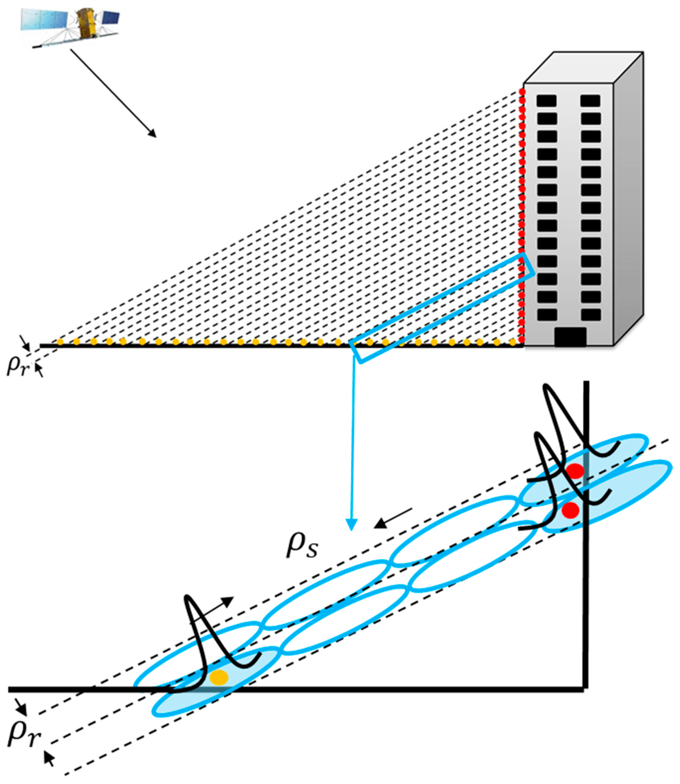
The spatial resolution in the height direction, orthogonal to the ground plane, depends on the elevation resolution, orthogonal to the range, which discriminates the scatterers such as that on ground and on the wall of building in Figure 2. The spatial resolution in the height direction also depends on the range resolution that can discriminate the scatterers such as the adjacent scatterers on the wall of the building in Figure 2, which is related to the transmitted signal bandwidth [10]. However, the current single-look or multi-look TomoSAR methods mentioned above are based on an azimuth-range pixel (Figure 1) or their neighbor pixels to reconstruct the reflectivity function along the elevation direction and to provide resolution power for elevation. Therefore, limited by the elevation resolution, these approached cannot discriminate scatterers that are located at very close elevation coordinates but at different ranges, such as the adjacent scatterers on the wall of building (Figure 3). To distinguish such scatterers, a better method is to enhance the range resolution if a larger signal bandwidth is available. This is possible because the sensed reflectivity’s spectrum band in multi-baseline acquisition is larger than that of a single pass [19]. Therefore, the range resolution may first be improved and then TomoSAR can be implemented. However, a problem that occurs is that the range resolution improvement influences the phase information, which results in incorrect inversion results for elevation.

Another way to enhance range resolution is the use of 2D spectrum analysis techniques [20,21,22,23,24], but in practice, a uniform distribution baseline is required, or else these techniques cannot be used. Moreover, the high-resolution analysis techniques are generally based on the computation and characterization of the signal covariance matrix. These approaches cannot be implemented in practice due to the high dimension of the resulting signals, whose covariance matrix estimation would require an extremely high number of samples. This serious limitation was overcome in this study through the use of estimation techniques that estimate the parameters or signals with a large dimension, but a sparse structure, i.e., composed of a small number of contributions. Considering that the elevation signals of urban areas are sparse in the object domain, the range-elevation signals to be reconstructed also are sparse, which is a key prerequisite for Compressive Sensing (CS) theory [25,26,27,28]. To overcome the limitations mentioned above, we propose applying the CS technique to super-resolution reconstruction, both for range and elevation. Unlike existing approaches, the CS-based range-elevation dimensional TomoSAR, or the CS 2D TomoSAR method, can not only provide reconstruction with a low number of irregularly spaced acquisitions, but can also improve the range and elevation resolution.

This paper is outlined as follows. In Section 2, a general tomographic SAR imaging model and the CS methodology in SAR tomography are outlined, and the 2D tomographic SAR imaging model as well as the proposed CS 2D TomoSAR method are derived. The datasets used are listed in Section 3. In Section 4, the performance of our approach is demonstrated using simulated experiments and by MB-PolInSAR datasets acquired by RADARSAT-2 at C-band over Lanzhou, China. Finally, conclusions are drawn in Section 5.

2. Methodology

2.1. One-Dimensional Tomographic SAR Imaging Model

Assume $M$ SAR images are available over the subject area. The $m$th image after the MB-InSAR acquisition geometry is shown in Figure 1, in which the SAR sensors move along $M$ parallel orbits over the same area, for sake of simplicity. Without loss of generality, let us consider $m_1$th orbit to be a reference orbit with a look angle of $\theta$. Using this process, the reference azimuth $x$ is the along-track direction of the $m_1$th orbit, the reference range $r$ is its across-track direction, and the reference elevation direction $s$ is orthogonal to the slant plane which is the $\left(x,r\right)$ plane. The baseline distance between the reference orbit and the $m$th position, noted as $b_m$, can be decomposed into $b_{//m}$, a component parallel to the slant-range direction, and a perpendicular component $b_{\perp m}$, aligned with the cross-range direction. After SAR imaging processing of echo signals acquired from each pass and coregistration of these data to the reference data, a stack of range-azimuth focused images are generated. The focused complex-valued images $u_m\left(x^{\prime },r^{\prime }\right)$ of an azimuth-range cell $\left(x^{\prime },r^{\prime }\right)$, for the $m$th acquisition, can be modeled in the following form [3]:

$$u_m\left(x^{\prime },r^{\prime }\right)=\iint dxdrf\left(x^{\prime }-x,r^{\prime }-r\right)\int ds\gamma \left(x,r,s\right)\exp \left[-j\frac{4\pi }{\lambda }{R}_m\left(r,s\right)\right],m=1,\dots ,M$$

(1)

where $\lambda$ is the operating wavelength, $f(·)$ is the postfocusing (compressed) 2D point spread function (PSF), $\gamma (·)$ is the 3D scene reflectivity function so the integrals are extended to the illuminated scene, and $R_m(·)$ is the distance between the target and sensor.

Without any spectral windowing, the postfocusing PSF $f(·)$ is:

$$f\left(x^{\prime },r^{\prime }\right)=\sin \mathrm{c}(\frac{x^{\prime }}{{\rho }_x})\sin \mathrm{c}(\frac{r^{\prime }}{{\rho }_r})$$

(2)

where ${\rho }_x$ and ${\rho }_r$ are the azimuth and range resolution, respectively. In the current tomographic SAR imaging model, we assumed the postfocusing PSF would approximate an ideal 2D Dirac function. So, for a fixed azimuth-range cell $\left(x_1^{\prime },r_1^{\prime }\right)$, the calculation of triple integral in Equation (1) can be transformed into a single integral, only in the vertical direction as follows:

$$u_m\left(x_1^{\prime },r_1^{\prime }\right)=\underset{-\mathsf{\Delta }s/2}{\overset{\mathsf{\Delta }s/2}{\int }}\gamma \left(s\right)\exp \left[-j\frac{4\pi }{\lambda }{R}_m\left(s\right)\right]ds$$

(3)

where $\mathsf{\Delta }s$ is the extent of the illuminated scene in the vertical direction. Through deramping and approximation by discretizing the continuous reflectivity function along s, in the presence of noise $\epsilon$, the discrete space system model of Equation (3) can be written as [3]:

$$\mathrm{g}={\mathit{R}}_e\gamma +\epsilon$$

(4)

where $\mathrm{g}$ is the column vector with $M$ elements

$$g_m=\exp \left[j\frac{4\pi }{\lambda }{R}_m\left(0\right)\right]{\int }_{-\mathsf{\Delta }s/2}^{\mathsf{\Delta }s/2}\gamma \left(s\right)\exp \left[-j\frac{4\pi }{\lambda }{R}_m\left(s\right)\right]ds.$$

${\mathit{R}}_e$ is an $M\times N$ mapping (steering) matrix with ${\mathit{R}}_{em\times n}=\exp \left(-j2\pi {\xi }_m{s}_n\right)$, where:

$${\xi }_m=\frac{2}{\lambda }\frac{b_{\perp m}}{r}$$

(5)

is the spatial (elevation) frequency. $\gamma$ is the discrete reflectivity vector with $N$ elements ${\gamma }_n=\gamma \left(s_n\right)$. $s_n$ (l = 1, …, $N$) denotes the discrete elevation position. This results in the 1D tomographic SAR imaging model.

2.2. Two-Dimensional Tomographic SAR Imaging Model

In this section, we will derive the 2D TomoSAR imaging model. From Equations (1) and (2), after deramping the 2D SAR image $u\left(x^{\prime },r^{\prime }\right)$ can be modeled in the following form:

$$u\left(x^{\prime },r^{\prime }\right)=\iint dxdr\sin \mathrm{c}(\frac{r^{\prime }-r}{{\rho }_r})\sin \mathrm{c}(\frac{x^{\prime }-x}{{\rho }_x})\int ds\gamma \left(x,r,s\right)\exp \left[-j\frac{4\pi }{\lambda }R\left(r,s\right)\right]$$

(6)

Here, we only assumed the function associated to the azimuth variables $x^{\prime }$ in the postfocusing PSF $f\left(x^{\prime },r^{\prime }\right)$ to approximate an ideal Dirac function. In other words, the azimuth dependence of $u$ and $\gamma$ can be omitted. Accordingly, we shifted from a 3D to a 2D estimation problem in the range direction r and elevation direction s. Thus, Equation (6) becomes :

$$u\left(r^{\prime }\right)=\int \sin \mathrm{c}\left(\frac{r^{\prime }}{{\rho }_r}\right)\ast (\gamma \left(r^{\prime },s\right)\exp \left[-j\frac{4\pi }{\lambda }R\left(r^{\prime },s\right)\right])ds$$

(7)

where $\ast$ is convolution. So, the Fourier transform of $u\left(r^{\prime }\right)$ is given by [29]:

$$U\left(f_r\right)=\int \mathrm{rect}(\frac{f_r}{B_W})\mathcal{T}\left(f_r+f_0,s\right)ds$$

(8)

where

$$\mathrm{rect}\left(x\right)=\{\begin{array}{c}1,x\in \left[-\frac{1}{2},\frac{1}{2}\right]\\ 0,x\notin \left[-\frac{1}{2},\frac{1}{2}\right]\end{array}$$

(9)

$B_W$ is bandwidth of the SAR system, $f_0$ is the center frequency of the SAR system, and $\mathcal{T}(·)$ stands for the Fourier transform of $\gamma (·)$.

Moreover, we assumed that the range resolution is enhanced, which is ${\rho }_r/{\mathsf{\eta }}_r$ where ${\mathsf{\eta }}_r>1$, and then the Fourier transform of the 2D signal can be written as:

$$U^{{\mathsf{\eta }}_r}\left(f_r\right)=\int \mathrm{rect}(\frac{f_r}{{\mathsf{\eta }}_r{B}_W})\mathcal{T}\left(f_r+f_0,s\right)ds$$

(10)

Therefore, from Equations (8) and (10) we have

$$U\left(f_r\right)=U^{{\mathsf{\eta }}_r}\left(f_r\right)$$

(11a)

or

$$FT\left[u\left(r^{\prime }\right)\right]{|}_{f_r}=FT\left[u^{{\mathsf{\eta }}_r}\left(r^{\prime }\right)\right]{|}_{f_r}$$

(11b)

or

$$\iint \sin \mathrm{c}\left(\frac{r^{\prime }}{{\rho }_r}\right)\ast \left(\gamma \left(r^{\prime },s\right)\exp \left[-j\frac{4\pi }{\lambda }R\left(r^{\prime },s\right)\right]\right)\exp \left[-j2\pi f_r{r}^{\prime }\right]d{r}^{\prime }ds=\iint \sin \mathrm{c}(\frac{r^{\prime }}{{\rho }_r/{\mathsf{\eta }}_r})\ast (\gamma \left(r^{\prime },s\right)\exp \left[-j\frac{4\pi }{\lambda }R\left(r^{\prime },s\right)\right])\exp \left[-j2\pi f_r{r}^{\prime }\right]d{r}^{\prime }ds$$

(11c)

for any $f_r\in \left[-\frac{B_W}{2},\frac{B_W}{2}\right]$.

As with the previous analysis in Section 2.1, we assumed that the same stack of $M$ complex SAR datasets were acquired. For the image acquired along the generic $m$th orbit, its Fourier transform across the range direction can be obtained from Equation (8):

$$U_m\left(f_r\right)=\int \mathrm{rect}(\frac{f_r}{B_W})\mathcal{T}\left(f_r+f_0-\mathsf{\Delta }{f}_m,s\right)ds$$

(12)

where

$$\mathsf{\Delta }{f}_m=\frac{b_{\perp m}}{r^{\prime }tan\theta }{f}_0$$

(13)

We also assumed that the range resolution is in by ${\mathsf{\eta }}_r>1$ times. Then, for the Fourier transform of the $m$th image across range direction, we obtain from Equation (10):

$$U_m^{{\mathsf{\eta }}_r}\left(f_r\right)=\int \mathrm{rect}(\frac{f_r}{{\mathsf{\eta }}_r{B}_W})\mathcal{T}\left(f_r+f_0-\mathsf{\Delta }{f}_m,s\right)ds$$

(14)

As before, for any $f_r\in \left[-\frac{B_W}{2},\frac{B_W}{2}\right]$, we have:

$$U_m\left(f_r\right)=U_m^{{\mathsf{\eta }}_r}\left(f_r\right),m=1,2,\dots ,M$$

(15)

For $K$ contiguous pixels ${\left\{u\left(r_k^{\prime }\right)\right\}}_{k=0}^{K-1}$ along the range direction, we have:

$$u\left(r_k^{\prime }\right)=\int \sin \mathrm{c}(\frac{r_k^{\prime }}{{\rho }_r})\ast (\gamma \left(r_k^{\prime },s\right)\exp \left[-j\frac{4\pi }{\lambda }R\left(r_k^{\prime },s\right)\right])ds,k=0,1,\dots ,K-1$$

(16)

Its discrete Fourier transform is given by:

$$U\left(f_r\right)=\sum _{k=0}^{K-1}u\left(r_k^{\prime }\right)\exp \left[-j2\pi \frac{k{f}_r}{K}\right],f_r=0,1,\dots ,K-1$$

(17)

After the range solution is enhanced by ${\mathsf{\eta }}_r>1$ times, for $K·{\mathsf{\eta }}_r$ contiguous pixels ${\left\{u\left(r_k^{″}\right)\right\}}_{k=0}^{K{\mathsf{\eta }}_r-1}$ along the range direction in the same area, its discrete Fourier transform is given by:

$$U^{{\mathsf{\eta }}_r}\left(f_r\right)=\sum _{k=0}^{K{\mathsf{\eta }}_r-1}u\left(r_k^{″}\right)\exp \left[-j2\pi \frac{k{f}_r}{K\times {\mathsf{\eta }}_r}\right],f_r=0,1,\dots ,K\times {\mathsf{\eta }}_r-1$$

(18)

From Equation (11), we let:

$$U^{{\mathsf{\eta }}_r}\left(f_r+\mathsf{\Delta }k\right)=U\left(f_r\right),f_r=0,1,\dots ,K-1$$

(19)

where $\mathsf{\Delta }k$ is any positive integer with $0\le \mathsf{\Delta }k\le K\left({\mathsf{\eta }}_r-1\right)$.

From Equations (15) and (19), for the image acquired along the generic mth orbit, we also have:

$$U_m^{{\mathsf{\eta }}_r}\left(f_r+\mathsf{\Delta }k\right)=U_m\left(f_r\right),f_r=0,1,\dots ,K-1$$

(20)

Equation (20) can be written in matrix notation:

$$\mathit{U}=\mathit{u}{\mathit{R}}_r$$

(21)

where $\mathit{U}$ is $M\times K$ matrix with

$$U=\left[\begin{array}{c}{U}_1\\ U_2\\ \begin{array}{c}⋮\\ U_M\end{array}\end{array}\right]$$

(22)

and

$$U_m=\left[U_m\left(1\right),U_m\left(2\right),\dots U_m\left(K-1\right)\right]$$

(23)

${\mathit{R}}_r$ is $\left(K\times {\mathsf{\eta }}_r\right)\times K$ matrix with

$${\mathrm{R}}_r^{f_{r}k}=\exp \left[-j2\pi \frac{f_{r}k}{K\times {\mathsf{\eta }}_r}\right],f_r=0,1,\dots ,K\times {\mathsf{\eta }}_r-1,k=0+\mathsf{\Delta }k,1+\mathsf{\Delta }k,\dots ,K-1+\mathsf{\Delta }k,$$

(24)

$\mathit{u}$ is $M\times \left(K\times {\mathsf{\eta }}_r\right)$ matrix with

$${\mathrm{u}}_{m{f}_r}={\mathrm{u}}_m\left(r_{f_r}^{″}\right)=\int \sin \mathrm{c}(\frac{r_{f_r}^{″}}{{\rho }_r/{\mathsf{\eta }}_r})\ast (\gamma \left(r_{f_r}^{″},s\right)\exp \left[-j\frac{4\pi }{\lambda }{R}_m\left(r_{f_r}^{″},s\right)\right])ds$$

(25)

From Equation (4), we know that:

$$\mathit{u}={\mathit{R}}_e\mathit{X}$$

(26)

where $\mathit{X}$ is N × $\left(K\times {\mathsf{\eta }}_r\right)$ unknown reflectivity matrix along range r and elevation s with

$${\mathsf{\gamma }}_{n,f_r}=\gamma \left(r_{f_r}^{″},s_n\right)$$

(27)

Thus, by replacing $\mathit{u}$ in Equation (21) with Equation (26), the 2D tomographic SAR imaging model can be obtained:

$$\mathit{U}={\mathit{R}}_e\mathit{X}{\mathit{R}}_r$$

(28)

The linear expression of Equation (28) is given by:

$$vec\left(\mathit{U}\right)={\mathit{R}}_r^T⨂{\mathit{R}}_{e}vec\left(\mathit{X}\right)$$

(29)

where $⨂$ is the Kronecker product and $vec(·)$ denotes the matrix to vector operator.

2.3. Compressive Sensing-Based 2D SAR Tomography Method

Based on the 2D TomoSAR imaging model derived above, we applied the compressive sensing technique to the 2D TomoSAR inversion. This novel approach of compressive sensing for sparse signal reconstruction [24,25,26,27,28] proposes that the signal $f\in {\mathrm{R}}^n$ can be measured from m corrupted linear measurements $b=\mathit{A}f+z$, where $\mathit{A}$ is an m × n sensing matrix, where m is typically much smaller than n, and z is an arbitrary and unknown vector of noise. The theory asserts that if f has approximately sparse representation in one basis $\mathsf{\Psi }$ that is also incoherent with $\mathit{A}$, then it is possible to recover $f$ from a small number of projections b by L₁ minimization:

$$\underset{\tilde{f}}{\min }{\Vert \mathsf{\Psi }\tilde{f}\Vert }_1,\mathrm{subject}\mathrm{to}{\Vert \mathit{A}\tilde{f}-b\Vert }_2\le \mathsf{\epsilon }$$

(30)

where $\mathsf{\epsilon }$ is an upper bound on the noise level. This minimization problem in Equation (30) can be solved using basis pursuit methods [30]. In this paper, the basis pursuit estimate is computed using the CVX tool (http://cvxr.com/cvx/).

For urban areas, the elevation signals to be reconstructed are sparse in the object domain. Then, the signal in the range-elevation plane is also assumed to be sparse. So, the sparse reflectivity profiles $vec\left(\mathit{X}\right)$ can be recovered based on the 2D TomoSAR imaging model in Equation (29) and the CS theory in Equation (30) in the presence of noise through $L_1$ minimization:

$${\min }_{l_1}\left(vec\left(\mathit{X}\right)\right)s.t.\Vert vec\left(U\right)-{\mathit{R}}_r^T⨂{\mathit{R}}_{e}vec\left(\mathit{X}\right)\Vert <\mathsf{\epsilon }$$

(31)

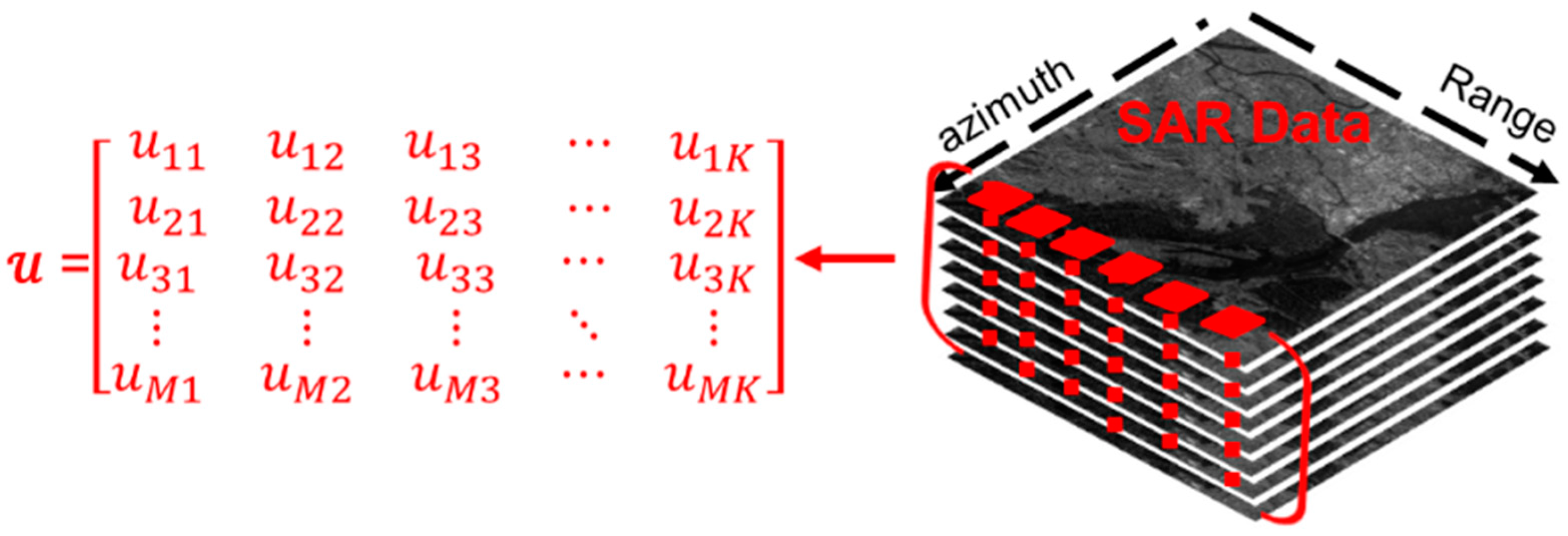
Notably, the matrix ${\mathit{R}}_r^T⨂{\mathit{R}}_e$ is a Kronecker product of two Fourier basis. Therefore, ${\mathit{R}}_r^T⨂{\mathit{R}}_e$ and identity orthogonal basis $I$ are maximally incoherent, which means that with overwhelming probability, ${\mathit{R}}_r^T⨂{\mathit{R}}_e$ obeys the restricted isometry property (RIP) to guarantee sufficiently sparse reconstruction in the presence of noise. The proposed CS 2D TomoSAR method can discriminate the scatterers not only along elevation direction but also along the range direction. The process of the method is shown in Figure 4, which shows that the main different with CS 1D TomoSAR is that the proposed CS 2D TomoSAR method use the Range-Doppler Signal $\mathcal{U}$ in a stack of SAR images (see Figure 5).

3. Datasets

To demonstrate the potential of the outlined approach, we used a stack of M = 7 focused C-band fully polarimetric SAR images of the urban site of Lanzhou, China, acquired by RADARSAT-2 from 9 July to 30 November 2012. The system parameters are shown in

Table 1. RADARSAT-2 SAR parameters.

Wavelength (m)	Range (km)	Incidence Angle	Total Baseline Span (m)	Azimuth Spacing (m)	Range Spacing (m)
0.0555	895	30°	405.87	5.17	4.73

. The spatial resolution was about 4.99 m in the slant range direction. The baseline information is reported in

Table 2. Baseline parameters.

Flight Date (2012)	Baseline (m) Flight Date of Master Image: 30 November 2012
9 July	141.12
2 August	251.43
26 August	−153.12
19 September	−138.31
11 October	−92.42
6 November	−132.73

. The master image was acquired 30 November 2012. The total baseline span was 405.87 m, resulting in a Rayleigh elevation resolution of 61.13 m. Before we completed the tomographic processing on the test site, a preprocessing of those MB-PolInSAR data was performed, including registration, flat earth phase removal, and atmospheric error phase removal [31].

4. Numerical Experiment

In this section, we investigate the performance of the CS 2D TomoSAR method in the following two ways: (1) we used some simulated experimental results based on our experimental parameters to investigate the advantages of the tomographic approach; and (2) real data experiments of the tomographic approach are presented.

4.1. Simulated Experiments

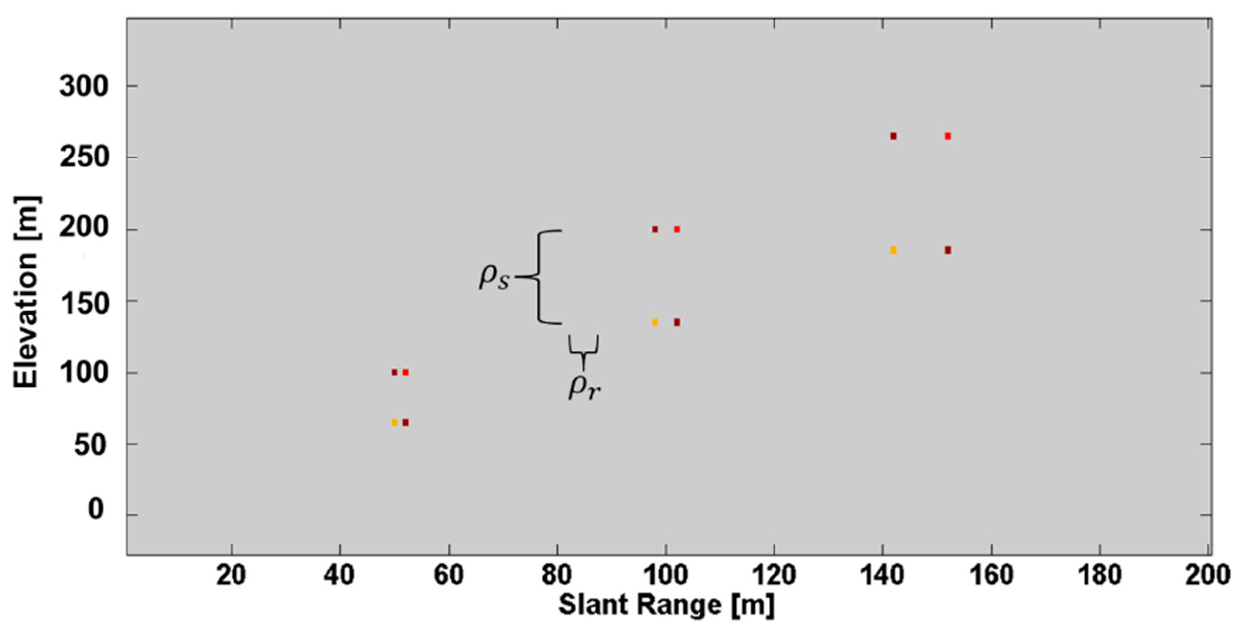
We first investigated the reconstruction performance of the technique. In simulated experiments, the signals with different reflectivity were simulated with seven acquisitions with a signal-to-noise ratio (SNR) of 20 dB. The acquisition parameters are displayed in Section 3 and the simulated original signals in the elevation-range plane are displayed in Figure 6. Three groups of simulated signals were used. In the second group, the range difference between the two scatterers that were located in difference range positions was equal to the range resolution, and the elevation difference between the two scatterers that were located in different elevation positions was equal to the elevation resolution. In the bottom-left of the figure, the range difference and the elevation difference are smaller than the range and elevation resolution respectively. In the upper-right of the figure, the range and elevation difference are larger than the range and elevation resolution, respectively.

We use the Fourier Beamforming, CS 1D TomoSAR, and CS 2D TomoSAR methods to recover the original signal with a SNR of 20 dB. Figure 7 shows the recovery signals with the Fourier Beamforming, CS 1D TomoSAR, and CS 2D TomoSAR methods in the elevation-range plane. For the Fourier Beamforming method, due to the limited elevation and range resolution power, the scatterers whose distance was less than or equal to the range and elevation resolution could not be distinguished (Figure 7a). 1D TomoSAR method could only discriminate the scatterers along the vertical direction; it could not discriminate those scatterers whose distance was less than or equal to the range resolution (Figure 7b). However, the CS 2D TomoSAR method achieved excellent resolution reconstruction of signals, both in the elevation and range directions (Figure 7c).

Next, we investigated the resolution power of the approach through simulation experiments to determine the closest range or elevation distance of two scatterers that could be discerned with a detection rate of more than 90%. We only analyzed the worst case (i.e., the signals have the same reflectivity) with the acquisition parameters provided in Section 3. In this experiment, the signals were simulated for scatterers with a SNR of 20 dB.

(1)

In first of all, we investigate the super-resolution power of the approach along range direction. We assume the two scatterers are in the same elevation but difference range position, i.e., the range distance between the two scatterers $\mathsf{\Delta }r>0$ m and the elevation distance between the two scatterers $\mathsf{\Delta }s=0$ m. Based on the CS 2D TomoSAR method, 500 independent numerical experiments were implemented. The detection rate of two scatterers with difference range distance $\mathsf{\Delta }r$ is shown in Figure 8a. We can see that the closest range distance of two scatterers such that they can be discriminated with a detection rate more than 90% is nearly 1.8 m. In other words, the range resolution of the CS 2D TomoSAR method in this case is 1.8 m, which is much smaller than the range resolution of the SAR data.

(2)

Then, we investigate the super-resolution power of the approach along elevation direction. We assume the two scatterers are in the same range but at different elevation positions, i.e., the range distance between the two scatterers $\mathsf{\Delta }r=0$ m and the elevation distance between the two scatterers $\mathsf{\Delta }s>0$ m. Based on the CS 2D TomoSAR method, 500 independent numerical experiments also were implemented. The detection rate of two scatterers with difference elevation distance $\mathsf{\Delta }s$ is shown in Figure 8b. We can see that the closest elevation distance of two scatterers such that they can be discriminated with a detection rate more than 90% is nearly 10 m. In the other word, the elevation resolution of the CS 2D TomoSAR method in this case is 10 m, which is also much smaller than the Rayleigh resolution in elevation. Moreover, we compared the elevation resolution of the CS 1D TomoSAR method with the one from our proposed method. Under the same experiments parameters and number of independent numerical experiments, the elevation resolution of the CS 1D TomoSAR method is 18 m, which is nearly twice that of the CS 2D TomoSAR method.

Finally, we investigated the estimation accuracy of our proposed method. In the experiments, the experimental parameters were as same as in the above experiments.

(1)

We first investigated the distance estimation accuracy of the two scatterers by fixing the elevation distance between the two scatterers. We analyzed the estimation accuracy under four different conditions, where the elevation distances between two scatterers $\mathsf{\Delta }s\mathrm{were}0$, 6, 10, and 30 m. Figure 9a shows that when $\mathsf{\Delta }s\mathrm{is}30$ m, the CS 2D TomoSAR method provided good estimation accuracy with a decreasing $\mathsf{\Delta }r$. This is because the elevation distance between the two scatterers was larger than the elevation resolution of the method. When $\mathsf{\Delta }s\mathrm{was}10$, which was equal to the elevation resolution of the CS 2D TomoSAR method, the estimation accuracy of the CS 2D TomoSAR method converged to a higher value with decreasing $\mathsf{\Delta }r$, due to the limited elevation resolution. When $\mathsf{\Delta }s\mathrm{was}0$ m, the estimation accuracy of the CS 2D TomoSAR method converged to a higher value with decreasing $\mathsf{\Delta }r$ until $\mathsf{\Delta }r\mathrm{was}1.8$ m. This was due to the limitation in the range resolution. Notably, the worst estimation accuracy of the CS 2D TomoSAR method occurred when $\mathsf{\Delta }s$ was 0 m, which was smaller than when $\mathsf{\Delta }s$ was 10 m. Moreover, when $\mathsf{\Delta }s\mathrm{was}6$ m, the worst estimation accuracy of the CS 2D TomoSAR method was between $\mathsf{\Delta }s=0$ m and $\mathsf{\Delta }s=10$ m, and the resolution power was also between $\mathsf{\Delta }s=0$ m and $\mathsf{\Delta }s=10$ m.

(2)

Then, we investigated the distance estimation accuracy of the two scatterers by fixing the range distance between the two scatterers. We also investigated the analysis results of the estimation accuracy under four different conditions, where the range between the two scatterers ($\mathsf{\Delta }r$) were 0, 1, 1.8, and 2.4 m. Figure 9b shows that when $\mathsf{\Delta }r\mathrm{was}2.4$ m, the CS 2D TomoSAR method provided good accuracy with decreasing $\mathsf{\Delta }s$. This is because the range distance between the two scatterers was larger than the range resolution of the method. When $\mathsf{\Delta }r\mathrm{was}1.8$ m, which was equal to the range resolution of the CS 2D TomoSAR method, the estimation accuracy of the CS 2D TomoSAR method converged to a higher value with decreasing $\mathsf{\Delta }s$, due to a limited elevation resolution. When $\mathsf{\Delta }r\mathrm{was}0$ m, the estimation accuracy of the CS 2D TomoSAR method also converged to a higher value with decreasing $\mathsf{\Delta }s$ until $\mathsf{\Delta }s$ was 10 m, because of the limitation in the elevation resolution. Notably, the worst estimation accuracy of the CS 2D TomoSAR method was when $\mathsf{\Delta }r$ at 10 m was larger than with $\mathsf{\Delta }r$ at 1.8 m. Moreover, when $\mathsf{\Delta }r$ was 1 m, the worst estimation accuracy of the CS 2D TomoSAR method was between $\mathsf{\Delta }r=0$ m and $\mathsf{\Delta }r=1.8$ m, and the resolution power was also between $\mathsf{\Delta }r=0$ m and $\mathsf{\Delta }r=1.8$ m. We also compared the estimation accuracy of the CS 1D TomoSAR method with our proposed method. Under the same experimental parameters and number of independent numerical experiments, the estimation accuracy of CS 1D TomoSAR method was always worse than that of the CS 2D TomoSAR method.

4.2. Real Data Experiments

This section is devoted to reporting the tomographic results of our method using the real data introduced in Section 3. In addition to facilitating the performance of the CS 2D TomoSAR method, we used the CS 1D TomoSAR method to compare with the new method.

4.2.1. Tomographic Profiles

To provide an example of how the CS 2D TomoSAR method can be used, we performed tomographic processing for 96 contiguous range positions (the yellow dashed line segment in the test zone shown in Figure 10) on the stack of seven focused and coregistered C-band HH channel SAR images in Lanzhou, China. From the optical image in Figure 10, some large oil storage siloes are in this scene, and those man-made targets can be easily recognized in the SAR image (Figure 10b). Moreover, those objects have good coherence (Figure 10c). From Figure 10, only one oil storage silo is on the yellow line. Figure 10e shows the close-up photo of the oil storage silo on the test line. The height of the storage silo is 26 m, which was measured by a hand-held laser range finder in field experiments. The direction of illumination of the microwave is from left to right. So, on the yellow line section, the scatterers on the façade that face the illumination will be reconstructed.

Figure 11 shows the reconstruction profile results of the test line in the elevation and range directions. Figure 11a is the result of the CS 1D TomoSAR method, Figure 11b,c are the results of the CS 2D TomoSAR method with the range resolution enhanced by two-fold and 1.5-fold, respectively. These results are consistent with our expectations from the tomographic processing of the elevation-range section considered, i.e., there is a sequence of reconstructed façade scatterers facing to the illumination in all the results. However, a few of the reconstructed scatters from the ground were found because the coherence of the signals from ground were low (Figure 10b). Due to the overlay, the sequence of the reconstructed façade scatterers was tilted. To present a more immediate view of the results, coordinate transformation from the range to ground distance was implemented. The red, yellow, and blue rectangles in Figure 11d compare the detailed reconstruction results between the CS 1D TomoSAR and CS 2D TomoSAR methods. Through comparing the two results in Figure 11a,b, due to the influence of the range resolution, the number of the façade scatterers reconstructed by CS 1D TomoSAR method was very small, and by improving the range resolution by using the CS 2D TomoSAR method, more scatterers were located very close to the elevation coordinates, but at different range coordinates, were separated. Moreover, from the tomogram of the test line obtained with the CS 2D TomoSAR method, we calculated that the distance between the ground and roof scatterers was about 28.98 m. The true height of this building is 26.0 m. The height estimation error with our real data was 2.98 m and the relative error was 11.5%. For the CS 1D TomoSAR method, the distance between the ground and roof scatterers was about 29.94 m, which is somewhat larger than the inversion result of the CS 2D TomoSAR method.

From the results of the method, the estimation of the CS 2D TomoSAR method is shown to be effective.

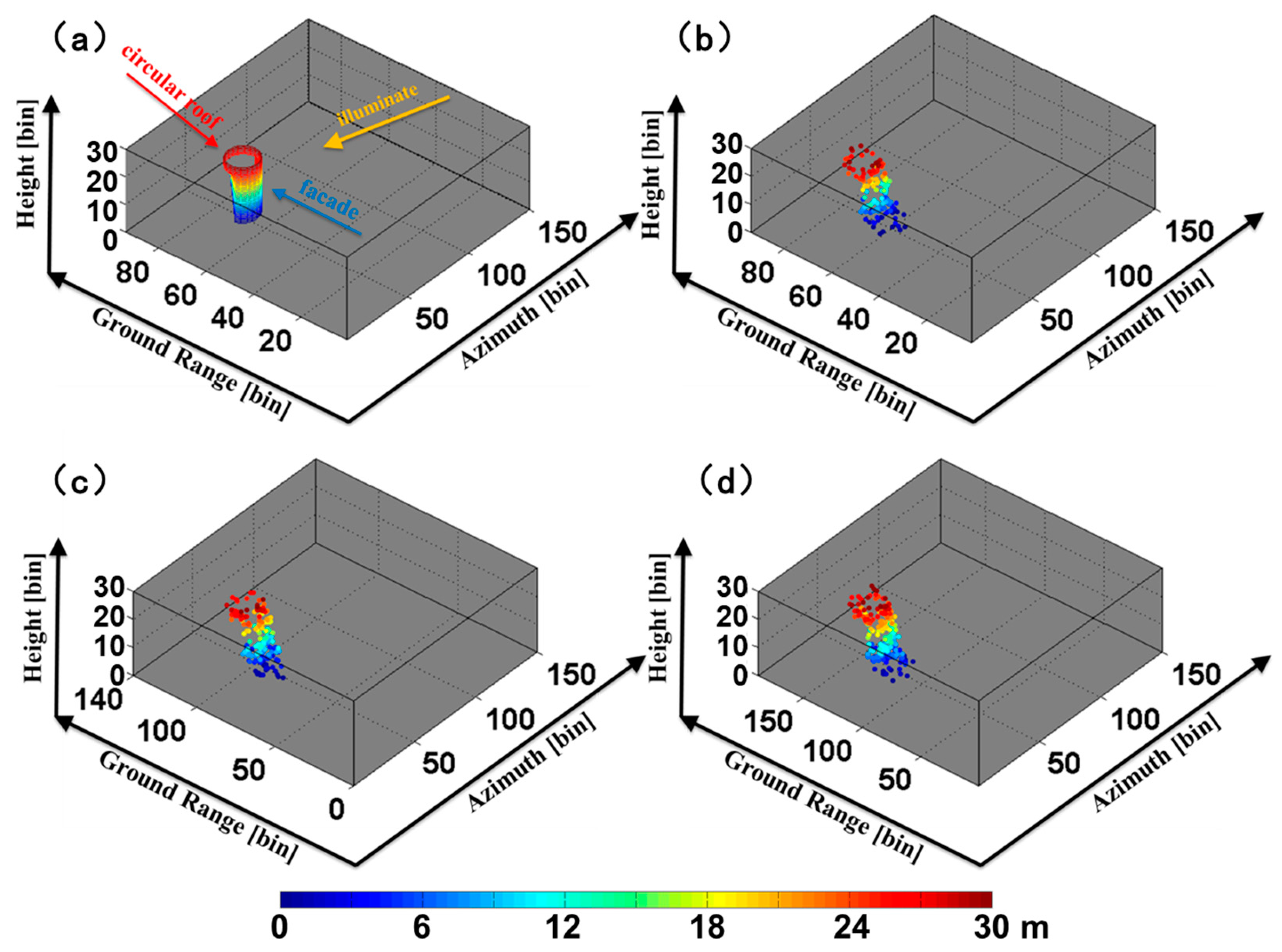
4.2.2. 3D View of the Building

To demonstrate the potential of the CS 2D TomoSAR method for urban area analysis, we performed tomographic processing on a building (Figure 10d). This target was selected because the coherence image of the target was structurally complete. Figure 12a shows a 3D schematic representation of the building. The target building has two parts: one façade facing the illumination and a circular roof. The back façade was missed because the microwave is blocked by the front façade. Figure 12b,d show the 3D visualization of the scatterers reconstructed with SAR tomography on the target building. Figure 12b is the result of the CS 1D TomoSAR method, and 487 scatterers were reconstructed. Figure 12c,d are the results of the CS 2D TomoSAR method with the range resolution enhanced by 1.5 times and 2 times, respectively. The results are consistent with the 3D schematic representation of the building. As before, with the improvements in range resolution, more scatterers on the target were reconstructed by the CS 2D TomoSAR method and nearly 691 and 832 scatterers were reconstructed where the range resolution was enhanced by 1.5 times and 2 times, respectively. Figure 13 shows a 3D visualization of the scatterers reconstructed with SAR tomography on the building zone. By using the CS 1D TomoSAR method, 7316 scatterers were reconstructed. However, when the range resolutions were enhanced by 1.5 times and 2 times by using the CS 2D TomoSAR method, 9709 and 12,205 scatterers were reconstructed, respectively.

From the results of the method, the CS 2D TomoSAR method provides more detailed information about the buildings than traditional 1D TomoSAR. With a large number of point clouds, the method is helpful for 3D modeling of urban areas.

5. Conclusions

In this paper, we proposed a CS-based 2D TomoSAR method. Based on an assumption that the signals in the range-elevation plane are simultaneously sparse, this method allows the joint recovery of the reflectivity range-elevation profiles. The CS 2D TomoSAR method enables the excellent vertical resolution by simultaneously using an additional synthetic aperture for elevation and a wider range spectrum, which is an important advantage over the 1D TomoSAR method.

The simulated experiments show that, compared to the 1D spectrum analysis methods, the CS 2D method has two main advantages: (1) The technique significantly enhances the resolution in the vertical direction. Unlike 1D spectrum analysis methods that are limited by the elevation resolution, the high resolution power of the CS 2D method depends on the range resolution that is much higher than the elevation resolution. The scatterers can be separated by this approach, provided that their distance along the horizontal direction is larger than the range resolution. (2) The technique also can significantly improve the estimate accuracy.

Real data experiments showed that the CS-based 2D TomoSAR method can be successfully employed to reconstruct scatterers in urban areas. The 2D TomoSAR method not only has better performance for height estimation but also can provide more 3D backscattering information than the CS-based 1D TomoSAR method.

References

- Reigber, A.; Moreira, A. First demonstration of airborne SAR to-mography using multibaseline L-band data. IEEE Trans. Geosci. Remote Sens. 2000, 38, 2142–2152. [Google Scholar] [CrossRef]
- She, Z.; Gray, D.A.; Bogner, R.E.; Homer, J. Three-dimensional SAR imaging via multiple pass processing. In Proceedings of the IEEE 1999 International Geoscience and Remote Sensing Symposium, Hamburg, Germany, 28 June–2 July 1999; pp. 35–38. [Google Scholar]
- Fornaro, G.; Serafino, F.; Soldovieri, F. Three-Dimensional Focusing With Multipass SAR Data. IEEE Trans. Geosci. Remote Sens. 2003, 41, 35–38. [Google Scholar] [CrossRef]
- Lombardini, F.; Reigber, A. Adaptive spectral estimation for multibaseline SAR tomography with airborne L-band data. In Proceedings of the 2003 IEEE International Geoscience and Remote Sensing Symposium, Toulouse, France, 21–25 July 2003; Volume 3, pp. 2014–2016. [Google Scholar]
- Guillaso, S.; Reigber, A. Polarimetric SAR tomography (POLTOMSAR). In Proceedings of the POLINSAR 2005 Workshop, Frascati, Italy, 17–21 January 2005. [Google Scholar]
- Gini, F.; Lombardini, F. Multibaseline cross-track SAR interferometry: A signal processing perspective. IEEE Aerosp. Electron. Syst. Mag. 2005, 20, 71–93. [Google Scholar] [CrossRef]
- Zhu, X.; Bamler, R. Very high resolution spaceborne SAR tomography in urban environment. IEEE Trans. Geosci. Remote Sens. 2010, 48, 4296–4308. [Google Scholar] [CrossRef] [Green Version]
- Huang, Y.; Ferro-Famil, L.; Reigber, A. Under-Foliage Object Imaging Using SAR Tomography and Polarimetric Spectral Estimators. IEEE Trans. Geosci. Remote Sens. 2012, 50, 2213–2225. [Google Scholar] [CrossRef]
- Budillon, A.; Evangelista, A.; Schirinzi, G. SAR tomography from sparse samples. In Proceedings of the 2009 IEEE International Geoscience and Remote Sensing Symposium, Cape Town, South Africa, 12–17 July 2009; pp. IV-865–IV-868. [Google Scholar]
- Budillon, A.; Evangelista, A.; Schirinzi, G. Three dimensional SAR focusing from multi-pass signals using compressive sampling. IEEE Trans. Geosci. Remote Sens. 2011, 49, 488–499. [Google Scholar] [CrossRef]
- Zhu, X.; Bamler, R. Tomographic SAR inversion by L1 norm regularization—The compressive sensing approach. IEEE Trans. Geosci. Remote Sens. 2010, 48, 3839–3846. [Google Scholar] [CrossRef]
- Zhu, X.; Bamler, R. Super-Resolution Power and Robustness of Compressive Sensing for Spectral Estimation With Application to Spaceborne Tomographic SAR. IEEE Trans. Geosci. Remote Sens. 2012, 50, 3839–3846. [Google Scholar] [CrossRef]
- Aguilera, E.; Nannini, M.; Reigber, A. Multi-Signal Compressed Sensing For Polarimetric SAR Tomography. In Proceedings of the 2011 IEEE International Geoscience and Remote Sensing Symposium, Vancouver, BC, Canada, 24–29 July 2011; pp. 1369–1372. [Google Scholar]
- Aguilera, E.; Nannini, M.; Reigber, A. Wavelet-based compressed sensing for SAR tomography of forested areas. In Proceedings of the 9th European Conference on Synthetic Aperture Radar, Nuremberg, Germany, 23–26 April 2012. [Google Scholar]
- Aguilera, E.; Nannini, M.; Reigber, A. Wavelet-Based Compressed Sensing for SAR Tomography of Forested Areas. IEEE Trans. Geosci. Remote Sens. 2013, 51, 5283–5295. [Google Scholar] [CrossRef] [Green Version]
- Aguilera, E.; Nannini, M.; Reigber, A. A data adaptive compressed sensing approach to polarimetric SAR tomography. In Proceedings of the 2012 IEEE International Geoscience and Remote Sensing Symposium (IGARSS), Munich, Germany, 22–27 July 2012; pp. 7472–7475. [Google Scholar]
- Liang, L.; Guo, H.; Li, X. Three-Dimensional Structural Parameter Inversion of Buildings by Distributed Compressive Sensing-Based Polarimetric SAR Tomography Using a Small Number of Baselines. IEEE J. Sel. Top. Appl. Earth Obs. Remote Sens. 2014, 7, 4218–4230. [Google Scholar] [CrossRef]
- Li, X.; Liang, L.; Guo, H.; Huang, Y. Compressive Sensing for Multibaseline Polarimetric SAR Tomography of Forested Areas. IEEE Trans. Geosci. Remote Sens. 2016, 54, 153–166. [Google Scholar] [CrossRef]
- Gatelli, F.; Guamieri, A.M.; Parizzi, F.; Pasquali, P.; Prati, C.; Rocca, F. The Wavenumber Shift in SAR Interferometry. IEEE Trans. Geosci. Remote Sens. 1994, 29, 855–865. [Google Scholar] [CrossRef]
- Li, J.; Stoica, P. An Adaptive Filtering Approach to Spectral Estimation and SAR Imaging. IEEE Trans. Signal Process. 1996, 44, 1469–1484. [Google Scholar]
- Li, J.; Liu, Z.S.; Stoica, P. 3-D target feature extraction via interferometric SAR. IEEE Proc.-Radar Sonar Navig. 1997, 144, 71–80. [Google Scholar] [CrossRef]
- Li, J.; Stoica, P.; Bi, Z.; Wu, R.; Zelnio, E.G. A Robust Hybrid Spectral Estimation Algorithm for SAR Imaging. In Proceedings of the Conference Record of the Thirty-Second Asilomar Conference on Signals, Systems & Computers, Pacific Grove, CA, USA, 1–4 November 1998; Volume 2, pp. 1322–1326. [Google Scholar]
- DeGraaf, S.R. SAR imaging via modern 2-D spectral estimation methods. IEEE Trans. Image Process. 1998, 7, 729–761. [Google Scholar] [CrossRef] [PubMed]
- Wang, Y.; Li, J.; Stoica, P. Spectral Analysis of Signals: The Missing Data Case; Morgan & Claypool Publishers: San Rafael, CA, USA, 2006. [Google Scholar]
- Candès, E. Compressive sampling. In Proceedings of the International Congress of Mathematicians, Madrid, Spain, 22–30 August 2006; Volume 3, pp. 1433–1452. [Google Scholar]
- Baraniuk, R.G. Compressive sensing. IEEE Signal Process. Mag. 2007, 24, 118–121. [Google Scholar] [CrossRef]
- Donoho, D.L. Compressed sensing. IEEE Trans. Inf. Theory 2006, 52, 1289–1306. [Google Scholar] [CrossRef]
- Candès, E.; Romberg, J.; Tao, T. Robust uncertainty principles: Exact signal reconstruction from highly incomplete frequency information. IEEE Trans. Inf. Theory 2006, 52, 489–509. [Google Scholar] [CrossRef]
- Cumming, I.G.; Wong, F.H. Digital processing of synthetic aperture radar data. Artech House 2005, 1, 3. [Google Scholar]
- Chen, S.S.; Donoho, D.L.; Saunders, M.A. Atomic decomposition by basis pursuit. SIAM J. Sci. Comput. 1998, 20, 33–61. [Google Scholar] [CrossRef]
- Berardino, P.; Fornaro, G.; Lanari, R.; Sansosti, E. A New Algorithm for Surface Deformation Monitoring Based on Small Baseline Differential SAR Interferograms. IEEE Trans. Geosci. Remote Sens. 2002, 40, 2375–2383. [Google Scholar] [CrossRef]
Figure 1.
One-dimensional (1D) synthetic aperture radar tomography (TomoSAR) model.
Figure 2.
The spatial resolution in the vertical direction depends on the elevation and range resolution.
Figure 3.
The elevation resolution in an azimuth-range cell.
Figure 4.
Flow diagram of compressive sensing-based two-dimensional range-elevation TomoSAR (CS 2D TomoSAR) method.
Figure 5.
Range-Doppler Signal in the range-elevation plane.
Figure 6.
Original signal in the range-elevation plane.
Figure 7.
Reconstruction signal in the range-elevation plane: (a) Fourier Beamforming; (b) CS 1D TomoSAR method; and (c) CS-2D-TomoSAR method.
Figure 8.
Detection rate as a function of (a) at = 0 m and (b) at = 0 m.
Figure 9.
Estimation accuracy of the distance between two scatterers as function of (a) ∆r at ∆s of 0, 6, 10, and 30 m, and (b) ∆s at , 1, 1.8, and 2.4 m.
Figure 10.
Experiments on test area: (a) Google Earth image; (b) SAR image; (c) coherence image; (d) and (c) a zoom of target building in red rectangle in (a) and (b); and (e) target building (oil storage silo with a height of 26 m) on the test line.
Figure 11.
Elevation-range sections of tomographic reconstruction over the test line, obtained with (a) CS 1D TomoSAR method; (b) CS-2D-TomoSAR with the range resolution enhanced two-fold; and (c) CS-2D-TomoSAR with the range resolution enhanced 1.5-fold; (d) The comparison of the detailed reconstruction results between the CS 1D TomoSAR and CS 2D TomoSAR methods. The color is associated to the estimated scattering magnitude of objects.
Figure 12.
(a) 3D view of the target building and 3D visualization of the scatterers reconstructed with SAR tomography, after coordinate transformation from range to ground distance; obtained with (b) the CS 1D TomoSAR method, (c) CS-2D-TomoSAR with the range resolution enhanced 1.5-fold and (d) CS-2D-TomoSAR with the range resolution enhanced two-fold. The color is associated to the estimated height.
Figure 13.
Three-dimensional visualization of the building zone of the scatterers reconstructed with SAR tomography, after coordinate transformation from range to ground distance, obtained with (a) CS 1D TomoSAR method; (b) CS-2D-TomoSAR with the range resolution enhanced 1.5 times; and (c) CS-2D-TomoSAR with the range resolution enhanced two-fold. The color is associated to the estimated height.