2.2. Data Collection
A field campaign was conducted during August in 2006, which represents the peak of the growing season. A portable spectroradiometer (FieldSpec Pro FR®, Analytical Spectral Devices (ASD), Inc., Boulder, CO, USA) was used to collect
in situ radiance between 350 to 1,000 nanometers (nm). A subset of these radiance data were parsed from the original spectra, 1 nm wide bands ranging from 415 to 1,000 nm. This range was strategically selected as a number of previous investigations have highlighted the near infrared (NIR) region as possessing the greatest utility for distinguishing vegetative targets [
1,
2,
3,
4]. Viewing geometry utilized a 24 degree field-of-view (FOV) held approximately 1-meter above the target for measurements representing field-canopy conditions. The viewing geometry configuration approximately represents the spatial resolution current airborne hyperspectral sensors can achieve (~1m pixel). Therefore, this sampling scheme is representative of a typical configuration of airborne hyperspectral flights. Approximately 30-40 spectra were collected at nadir and averaged per sampling location to better capture inherent target variability.
Radiance measurements were taken of a Spectralon® reference panel (Labsphere, Inc., North Sutton, NH, USA) near-simultaneously with each plant spectra. A Lambertian reference panel was utilized for calibration. Sun-target-sensor geometry was repeated as best as possible under these difficult field conditions between 11:00-14:30 local time. Rapidly sequenced measurements were averaged over a homogeneous (one species) plot. The instrument was shifted within the patch during collection to capture inherent within species variability and ensure non-overlapping FOVs. This was repeated at four different patches for each species. During data acquisition, the sensor was first placed over the reference panel to record the panel-reflected radiance. Then the sensor was placed over the target to record the target-reflected radiance. Then, by ratioing the radiance measurements, surface reflectance factor was calculated. By definition, the term reflectance factor (Equation 1) is the ratio of radiant emittance of a target to that reflected into the same reflected-beam geometry and wavelength range by an ideal and diffuse standard surface irradiated under the same conditions [
9]:
where S
i is the angular distribution of all incoming radiance and S
r is the reflected radiance measured by the sensor for a given λ wavelength [
7].
In addition to the ASD spectral configuration, a baseline spectral library was created and re-sampled utilizing the band center/Full Width Half Maximum (FWHM) profiles emulating common airborne hyperspectral imagers (48 bands, avg. FWHM 5.8 nm). In addition, a second re-sampling was conducted that doubled the number of bands (95 bands, avg. FWHM 2.9 nm) to evaluate the impact of instrument configuration on selected bands. These two data sets emulate the FWHM of currently available airborne hyperspectral sensors (e.g., Compact Airborne Spectrographic Image (CASI)-1500).
Table 1.
Sampled species from each study area. E:Emergent, S:Submergent, Fl:Floating, G:Graminoin, F:Forb, Sr:Shrub, R:Rushes/Segdes.
Table 1.
Sampled species from each study area. E:Emergent, S:Submergent, Fl:Floating, G:Graminoin, F:Forb, Sr:Shrub, R:Rushes/Segdes.
| MUSKEGON | | U.S. 127 | |
|---|
| Eleocharis rostellata | E | Asclepias incarnata | F |
| Elodea canadensis | S | Cephalanthus occidentalis | Sr |
| Filamentous algae | Fl | Cyperus esculentus | R |
| Heteranthera dubia | S | Eleocharis rostellata | E |
| Iris versicolor | E | Leersia orxyzoides | G |
| Leersia orxyzoides | G | Lemna minor | Fl |
| Lemna minor | Fl | Najas sp. | S |
| Lythrum salicaria | E | Phalaris arundinacea (Green) | G |
| Myriophyllum spicatum | S | Phragmites australis | E |
| Nuphar lutea | Fl | Sagittaria latifolia | E |
| Nymphaea odorata | Fl | Salix nigra | Sr |
| Phragmites australis | E | Schoenoplectus pungens | R |
| Poa sp. | G | Scirpus sp. (1) | R |
| Polygonum hydropiperoides | F | Scirpus sp. (2) | R |
| Pontederia cordata | E | Soldago gigantea | F |
| Potamogeton crispus | S | Sparganium androcladum | E |
| Sagittaria latifolia | E | Typha latifolia | E |
| Salix nigra | S | | |
| Schoenoplectus tabernaemontani | E | | |
| Spaganium americanum | E | | |
| Typha angustifolia | E | | |
| Vallisnera americana | S | | |
2.4. Analysis
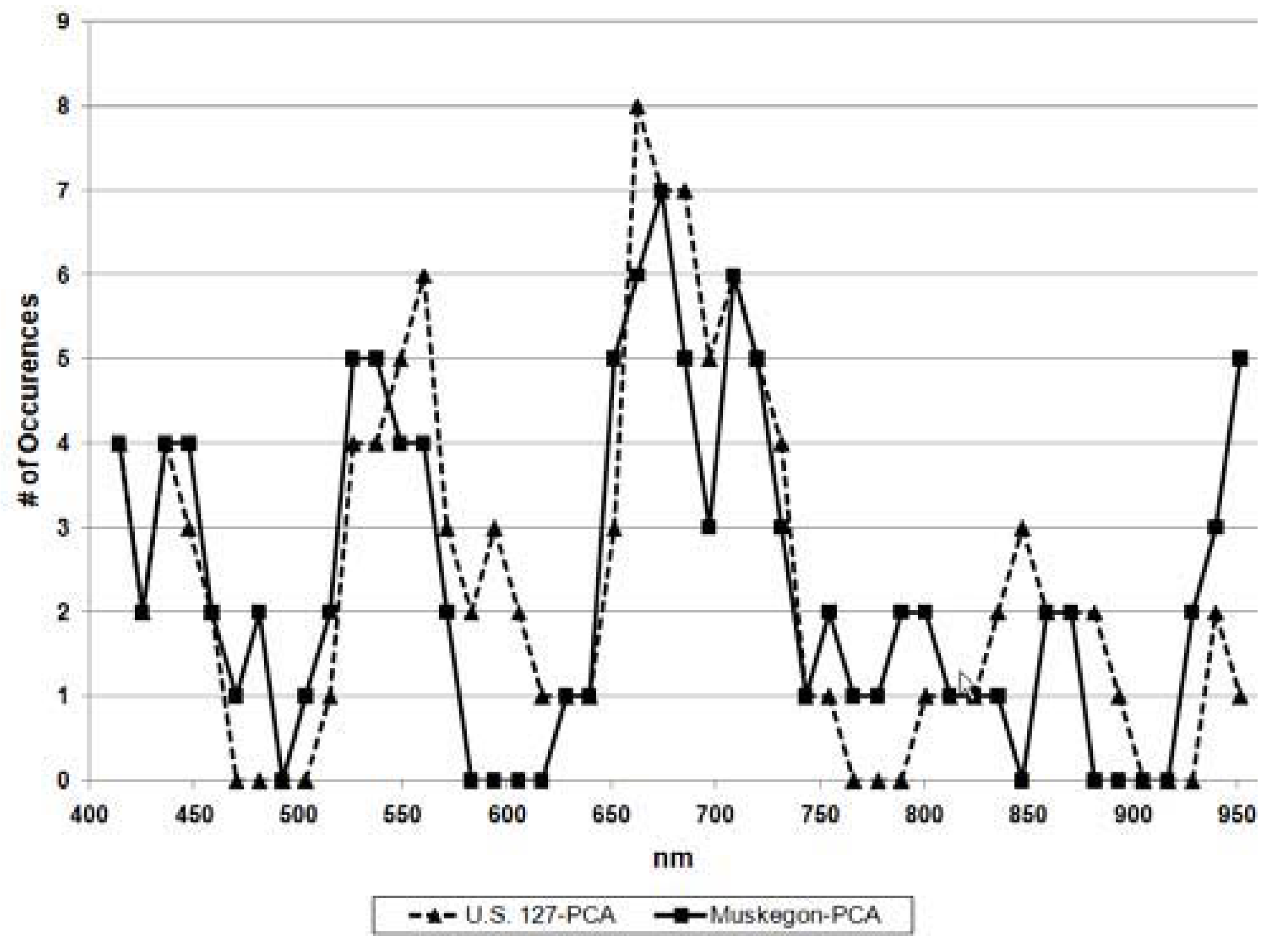
A set of extensive scripts were developed utilizing the MATLAB™ environment in order to transform the three data pools and their six subcategories into their principal components (i.e., dimensions). A single category was selected within the dataset to perform a principal components transformation. Band number was established as the independent variable in order to characterize the explanative power of each band with respect to the sampled, botanical community (i.e., dependent variable).
Correlation-based PCA references standardized input variables (i.e., correlation matrices) that have a mean of zero and a variance of one. Standardization tends to inflate the contribution of variables whose variance is small, and reduce the influence of variables whose dimensions are large. Covariance-based PCA, on the other hand, is typically used when the relative magnitudes of the variables are important because its un-standardized format enhances magnitude differences and reduces the potential for an insignificant variable to exert a strong influence on the results [
10]. Within the literature [i.e., 7-8], it remains unclear which methodology (covariance or correlation) was most applicable to band identification within the context of this research, so both were utilized. It was assumed that both provide a different, but meaningful, perspective.
Primary outputs of interest from PCA runs were eigenvalues and eigenvectors. Eigenvalues contain a synopsis of the percentage of the original data variance that is captured or explained by each principal component. Eigenvectors, which are by definition uncorrelated to each other and related to only one eigenvalue, provide information about data patterns within the new coordinate system. The eigenvalues, eigenvectors, and covariance/correlation matrices were further combined to yield component loadings (Equation 2). PCA component loadings represent a coefficient between each independent variable (i.e., band) and any one component:
where
b is each original band and
p is each principal component for covariance or correlation approach.
Stated differently, loadings measure the relative degree to which each original band explains the relationship between any one component and the body of dependant variables, in this case being botanical signatures. If any one component captured that portion of the overall data variance that was inherently related to the differentiation of these botanical signatures, then those bands loading highest on that component should also be well suited for botanical differentiation.
Although individual methods resulted in the identification of important loading values for an individual dimension, no method performed across the range of data. Thus, a more simplified approach to loading/band center selection was adopted. The top 10% positive and top 10% negative loading values were selected, when present. The 10% were calculated for each PC band, six for COR and 6 for COV based PCA. In some instances, especially the first dimensions, there are no negative loadings, so they are not present with respect to a single dimension.
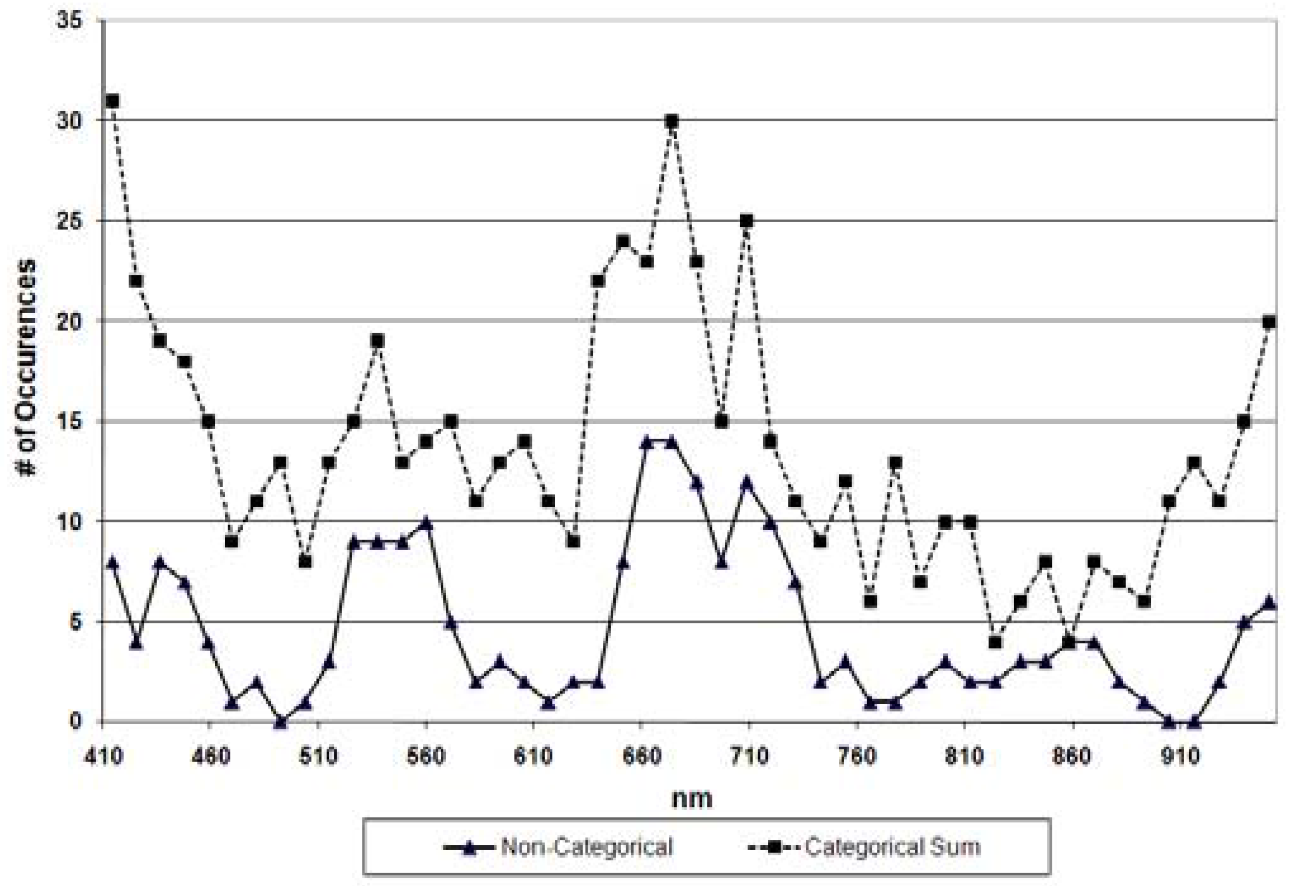
The number of output factors (i.e., dimensions) generated by PCA is typically held equal to the number of substantively meaningful independent patterns (extracted features) among the variables tested [
11]. In order to determine the dimensions deemed meaningful in this study, hyperspectral images of each study area was subjected to a PCA transformation. The resulting component images were systematically inspected in order to identify those dimensions that maintained landscape dependence. In both cases, the 7
th dimension and beyond were found to be noisy, and the features within the wetland were not discernable. Thus, PCA dimensions 1-6 were deemed meaningful for this investigation.
The identification of the meaningful dimensions and the band specific (i.e., 20% of the 48 or 95 bands) loading values are the baseline data matrices upon which further analyses were conducted. Histograms were generated for each baseline data matrix, depicting the relative frequency of selected component loading values vs. wavelength (i.e., band centers). This methodology allowed the visual inspection of the loading response-curves associated with the 12 extracted dimensions. The extracted dimensions refer to both PCA approaches. Fundamentally, the key band centers identified through the visual examination of loading histograms should be most applicable to the differentiation of the botanical community from which the PCA-based signatures were generated.
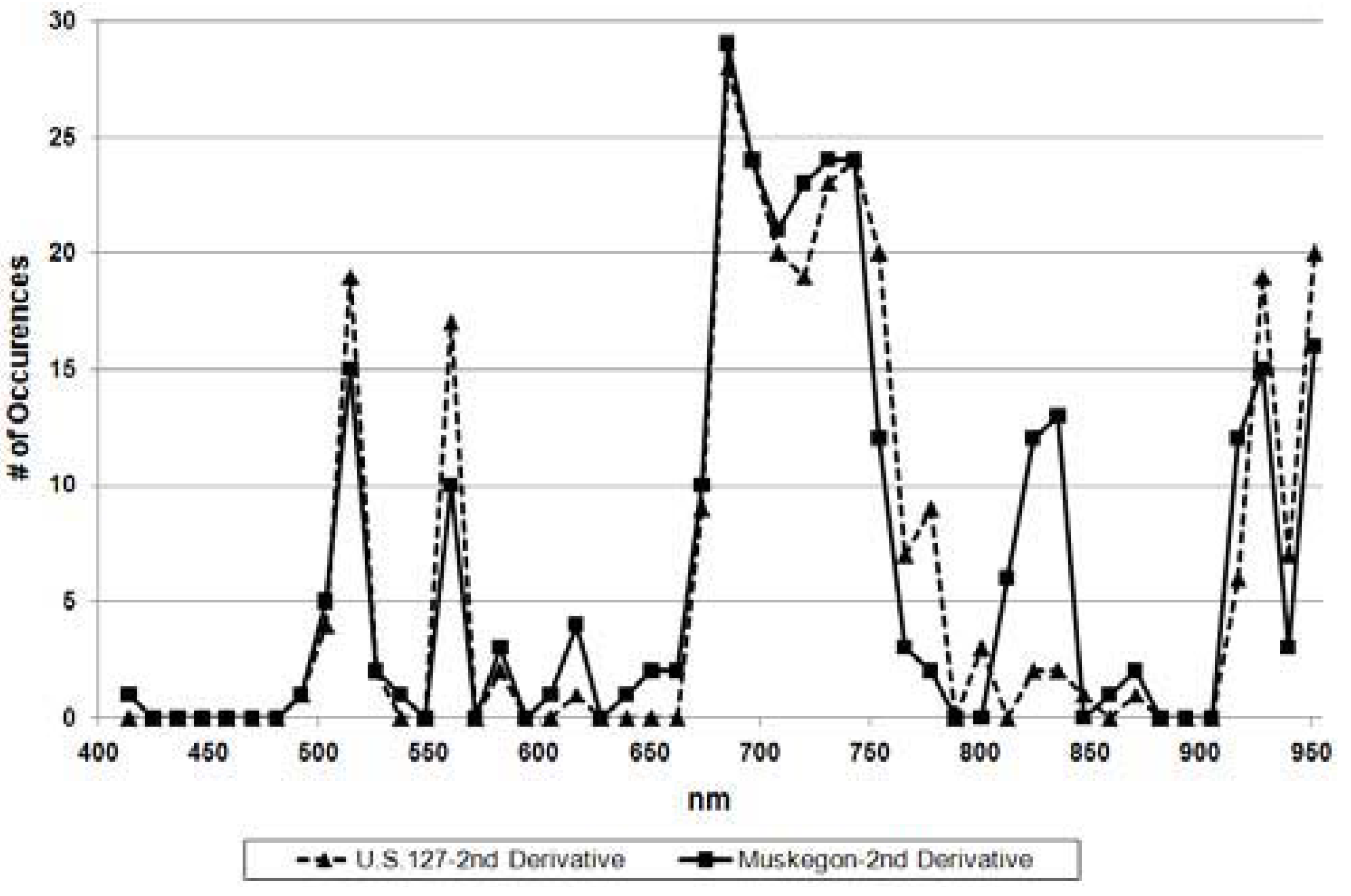
The PCA results were then compared to another common band selection tool, namely 2
nd derivative analysis (Equation 3). Derivative methodology has been used to distinguish wavelength locations where substantial inflection occurs [
3,
4]. In Becker
et al. [
3] and Torbick
et al. [
4], second derivative approximations identified seven wavelengths (685, 731, 939, 514, 812, 835, 823, 560 nm) using contiguous data covering the visible and NIR regions coastal wetlands of Lake Erie and Lake Huron, USA. A set of scripts were developed using a piecewise cubic spline to smooth a non-continuous/unsmoothed spectra in order to create a polynomial from which true second derivative values could be calculated at each band location. The five highest magnitude positive and negative values were selected to identify wavelengths possessing distinct diagnostic spectral change. This percentage was chosen because inspection of the data shows that derivatives and their paired wavelengths resulting from inflection points caused by system noise and not botanical sources were more frequent in the “middle” 80% of the data which has been shown to be a useful approach [
4]. The high magnitude values represent points of inflection that are located at the center of a reflectance (negative values capture convex features) and/or absorption feature (positive values capture concave features):
where d
1st is the 1
st derivative (line segment slope) and ρ is the percent reflectance factor at a given λ wavelength.

