1. Introduction
Obvious to everyone in the GIS sector, data acquisition, which reportedly accounts for 60-80% of the overall costs of a GIS project, plays an important role in GIS applications [
1]. The fact that a cost-effective and reliable GIS requires speed and accuracy in obtaining positions of objects is forcing administrators of GISs to find economical and productive solutions to data acquisition tasks. An answer is found in modern technology: GPS, especially RTK GPS. But, how good is it? Is it dependable; i.e. can it provide the same accuracy under any satellite configuration? Do we have to resort to static positioning mode of GPS? Can it reliably replace conventional terrestrial methods? This paper is an attempt to answer these questions that GIS specialists seem to be asking nowadays.
GPS aids in collecting individual points, lines and areas in any combination necessary for a mapping or GIS project. Furthermore, utilizing GPS one can form complex data dictionaries to accurately and efficiently collect attribute data. Thus, this makes GPS is a very effective tool for collecting both spatial and attribute data for use with GIS [
2].
GPS is also an effective tool for collecting control points for use in registering base maps when known points are not available and for geometric correction of high resolution satellite imagery. Acquisition of ground control points is particularly important for geometric correction of high resolution satellite images [
3]. Commercially available high resolution satellite images can be accurately rectified utilizing ground control points. However the accuracy of the results is dependent on the precision of the ground control points. The one of the most efficient and easiest ways to establish the three dimensional positions of the ground control points is to use GPS technology [
4].
Prior to the improvement of real time kinematic GPS with phase observations, real time positioning could be done with Differential GPS (DGPS) or by absolute positioning (AP or single point positioning). Both the DGPS and AP methods, which make use only of code pseudoranges, can produce positions with accuracies of 1-5 and 10-100 m, respectively. This is not acceptable for most GIS applications or any geodetic work, but they have been used generally for navigational purposes. However, static GPS measurements have started to be utilized for today’s most stringent GIS data requirements whether it be for effectively managing ambulances [
5] or urban digital cadastre [
6], in precision farming [
7], urban forest management [
84], urban disaster management [
9], or researches combining GPS and GIS [
10,
11,
12,
13].
The problems of obtaining high accuracy real time positions in the field have led the surveying community to develop a DGPS-like real time method called “Real Time Kinematic GPS (RTK GPS). The reason that RTK GPS can produce accuracies on the order of cm is that it uses phase observations. RTK GPS can be seen as somewhat like DGPS using phase observations. With the precision RTK GPS provides, it can or should often be utilized in any GIS or Remote Sensing project that requires a sub-decimetre accuracy for object or ground points such as in preparation of large scale plans (i.e. at scale of 1:1,000), zoning applications (also at scales of 1:1,000 or 1:2,000), building engineering structures such as canal and pipeline projects, vehicle monitoring, and road and railway projects and especially in providing necessary spatial data for geographical information systems or urban information systems [
14].
This paper investigates the internal and external accuracy abilities (performance) of RTK GPS for GIS applications. For this purpose, we have carried out tests to determine the suitability of this form of GPS positioning. Before we go on to detailed explanation of the tests we find it useful to briefly recount on background of real time kinematic GPS.
2. Real Time Kinematic GPS
The principle of RTK GPS is similar to that of DGPS, except that the RTK method uses and processes carrier phase observations for positioning. Since carrier phase observations produce more precise positions than code measurements, spatial positions obtained from RTK GPS are of better quality, with a precision in order of cm [
15].
As it is well known, staking out, positioning detail points and application works usually require much time and effort when traditional (terrestrial) equipment and procedures are used. With this relatively new method of positioning, however, these tasks can readily be carried out in much less time and with accuracy equal to (or even better than) that provided by the terrestrial methods. In order to obtain precise results from this method at least five satellites should be observed simultaneously, which may be considered as the only shortcoming. Nevertheless, the combination of GLONASS satellites with GPS has overcome this burden of tracking five satellites simultaneously in urban canyons crowded with high rise buildings or in densely tree populated areas [
16].
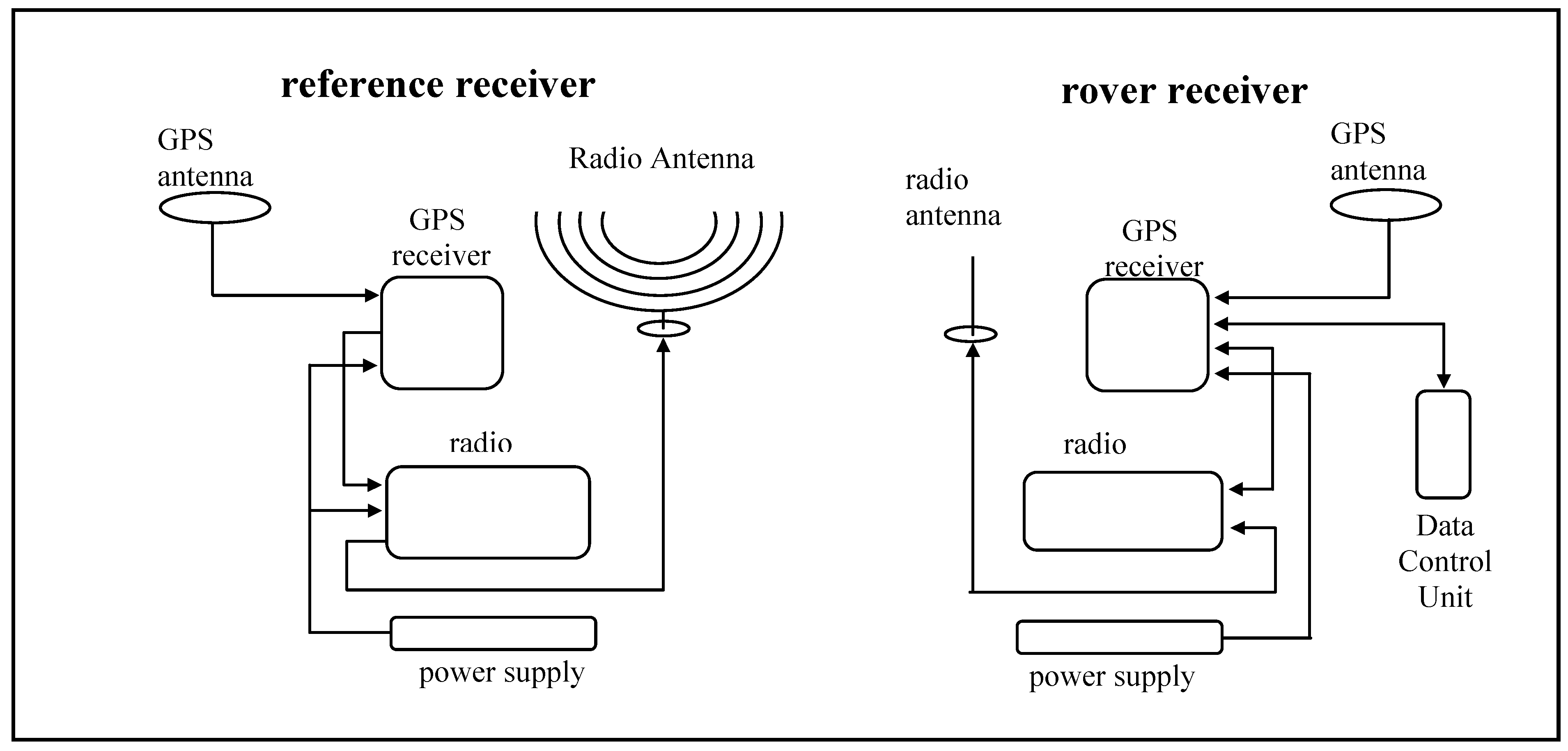
Figure 1.
A typical structure of RTK GPS.
Figure 1.
A typical structure of RTK GPS.
In RTK GPS mode, one GPS receiver placed on a station is kept static (reference station) during the whole observation session, while the other receiver moves among points (rover stations) whose spatial positions are to be determined. Both reference and rover stations are equipped with dual frequency receivers. Reference receiver has a radio transmitter aimed to send phase observation corrections to rover receiver which is also equipped with radio modem to establish a link with the reference station [
17]. The radio modem used in this system differs from the ones used in DGPS in that this radio modem has to update the correction data sent to a rover in 0.5-2 seconds. The volume of data sent by the reference receiver increases due to density of data update rate; as a result of this, RTK GPS requires the data link to have an optimal capacity of 2,400 bps (bytes per second) or at least 9,600 bps or even in some cases 19,200 bps. VHF of UHF bands in radio spectrum can provide bandwidths supporting this kind of data [
18].
Figure 1 illustrates a typical structure of RTK GPS.
In the RTK GPS technique, correction messages are sent to rovers in a certain format which every receiver manufacturer produces. In order to prevent the confusion that different data formats can cause, the Radio Technical Commission for Maritime Services, Special Committee 104 (RTCM SC-104) has published a standard format for broadcasting correction messages between reference and rover stations and this has been named as RTCM SC-104 [
19].
Naturally, the more reference and rover stations track satellites, the faster the ambiguity resolution gets and the more the positioning accuracies increase. Augmentation of GLONASS satellite signals with GPS signals can be used in this context.
Advantages of RTK GPS technique over other GPS techniques can be expressed as follows:
It does not require post-processing.
Coordinates of points measured in the field can be transformed to local coordinate systems in real-time, provided that a few points (at least three) whose coordinates are also known in local coordinate system are available.
It provides a reliable tool for positioning all points accurately. In conventional kinematic surveys in the case of (undetected) cycle slips or loss of lock in the reference station, kinematic positioning cannot be performed, whereas in RTK this is easily detected, the survey continues with a new integer ambiguity introduced and resolved in real-time.
Known points can accurately be staked out (on a cm level) in field in real-time.
By means of RTK, GPS receivers can readily be used as electronic tachometers (total stations) [
20].
Today RTK GPS is widely being used all over the world. Due to the increased productivity in terms of time and economics RTK GPS provides, in the near future this approach can and will surely replace the DGPS method and classical terrestrial positioning techniques.
3. Testing the Performance of RTK
In order to test the performance of RTK GPS, two different test configurations are considered, both within the borders of the Metropolitan City of Bursa, which is situated 100 km south of Istanbul, on the south coast of the Marmara Sea. In test 1, the internal accuracy (precision) of RTK GPS results is tested, while in test 2 the external accuracy is investigated. Three different cases are investigated in test 1, namely identical satellite configuration, different satellite configuration and different reference station, and two different cases in test 2, namely static GPS versus RTK GPS and conventional terrestrial techniques versus RTK GPS, so as to observe internal and external accuracies of the RTK GPS method.
Before giving the details of the tests conducted, the authors consider it useful to briefly explain the terms internal and external accuracies. The internal accuracy, also referred to as “precision”, is accuracy of measurement, obtained through repeated measurements with the same equipment. It does not describe the repeatability of a test result, but the sturdiness of the measurement instrument or its reading while measuring. According to DIN 55350-13 [
21], precision is the qualitative term for closeness of agreement between independent test results obtained under stipulated conditions. Precision depends only on the distribution of random errors and does not relate to the true value or the accepted reference value. In contrast to the term precision, accuracy is referred to as an “external” accuracy. Accuracy can be defined as the quality of the result and refers to how closely a measurement or observation comes to measuring a “true value”, since measurements and observations are always subject to error. According to DIN 55350-13, the term accuracy consists of two criteria, the precision and the trueness. Thus, the “internal” accuracy lies within the external accuracy [
22,
23].
3.1. Test 1: Observing Internal Accuracy
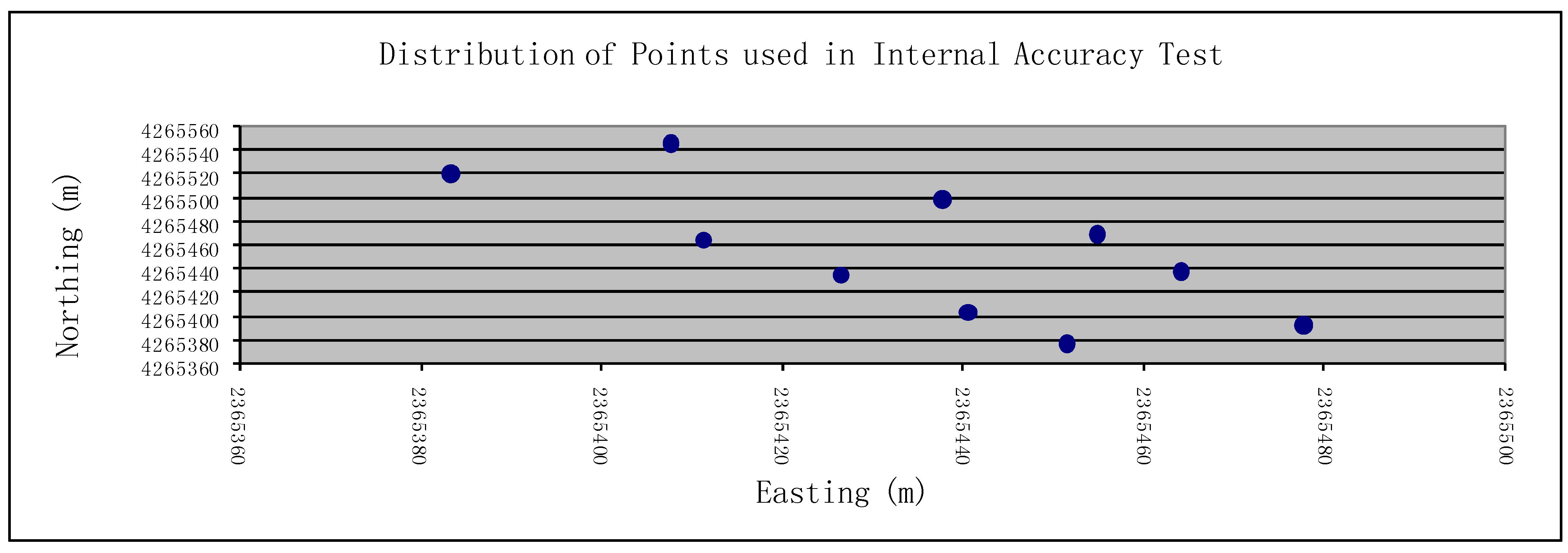
Ten arbitrary points were selected in a newly constructed park area in the Sogukkuyu district in the Metropolitan City of Bursa to test the positions obtained from RTK GPS, whether or not they are internally precise. Within this test, three different cases are taken into account to determine how precise the RTK GPS results are.
Figure 2 illustrates the distribution of points used in these three cases. Since the test field is densely populated with urban structures, as can easily be seen from the
Picture 1, the tests carried out make it possible to observe how precise results the method of RTK GPS will produce, especially in urban canyons. There observation cases are conducted on the selected test points, namely, Identical Satellite Configuration, Different Satellite Configuration and Different Reference Station. In all three cases all the RTK GPS measurements are conducted using two Zeiss GePos Experience dual frequency receivers with standard hardware and software and observing visible 6-8 satellites throughout the whole sessions and with PDOP values 1.5-2.4.
Figure 2.
Distribution of points used in internal accuracy test.
Figure 2.
Distribution of points used in internal accuracy test.
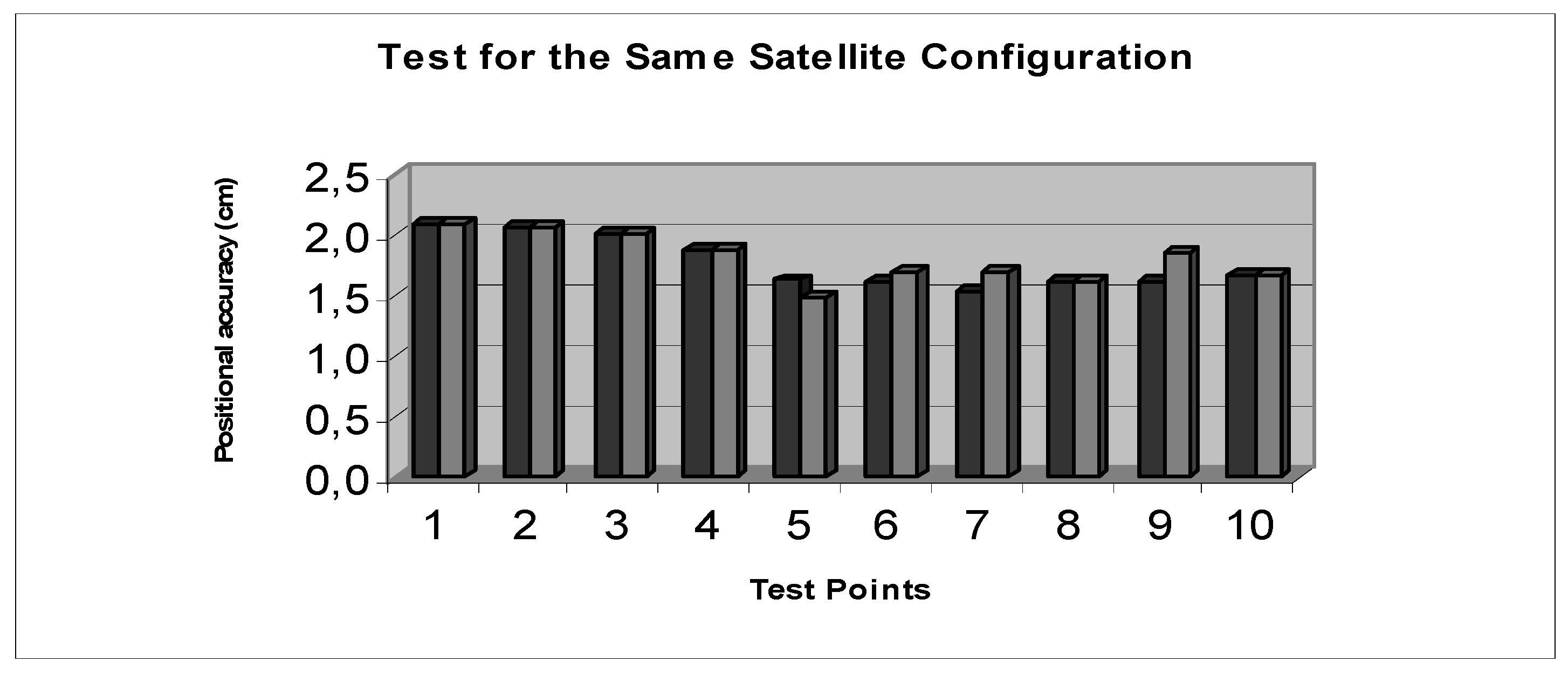
Case 1: Identical Satellite Configuration
GPS satellites are known to pass over the same point four minutes earlier next day on their routine orbits. For this reason it is of essence to note this daily four minute-offset in order to repeat the GPS observations the next day with the same number and configuration of satellites and, of course, the same DOP values. It is obvious that if the second period observations are repeated “n” days later, then the observations should be made 4 x n minutes earlier than the first period.
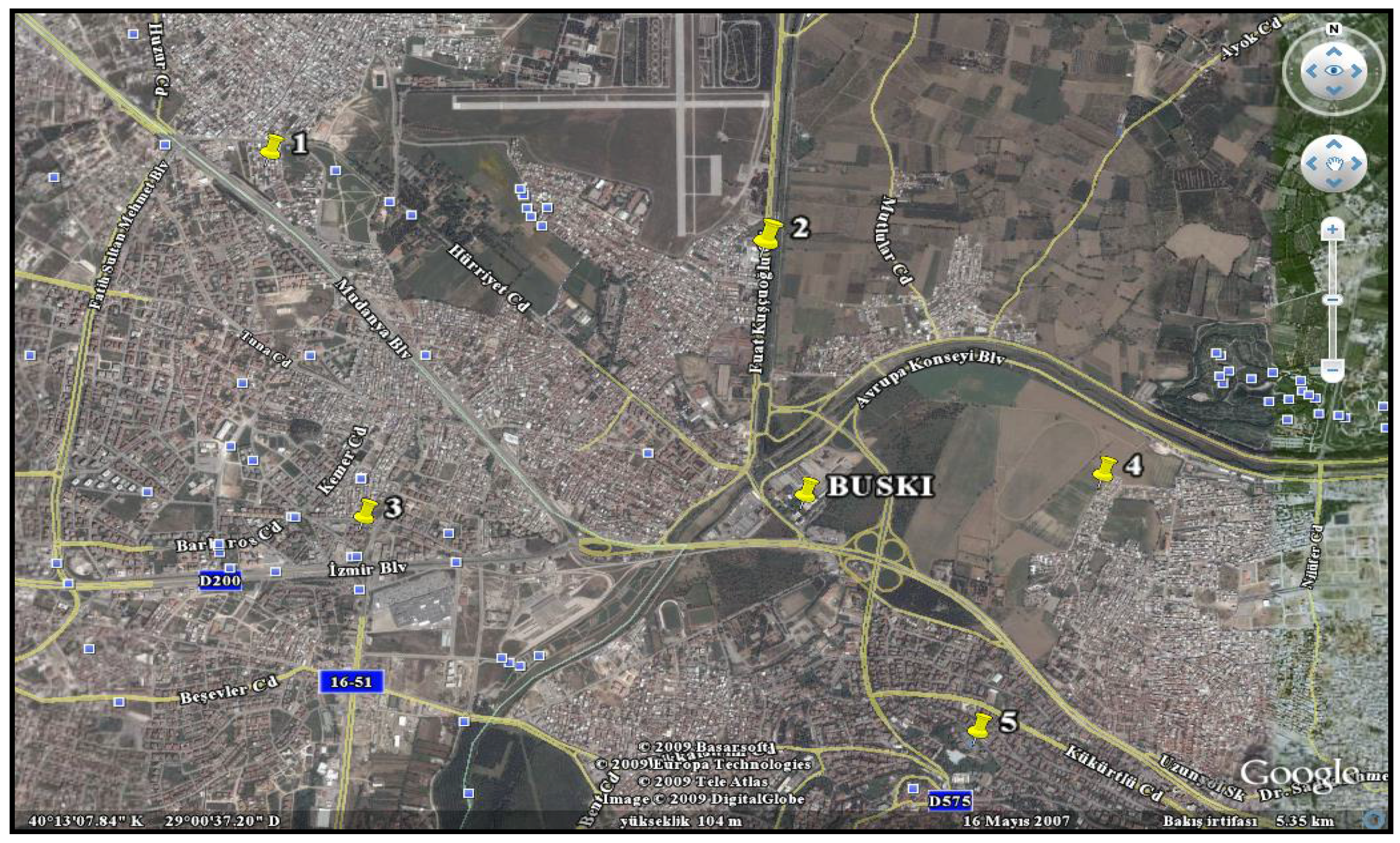
Bearing this in mind, for this test the second set of observations was made four minutes earlier on the next day than the first set. However, as a precaution measure the first day observations were carried out at each point with three different observation starting times, in case it were not possible to make observations at the exact time next day. The point 50960 on the roof of the BUSKI building (BUSKI is short for Bursa Metropolitan City Irrigation and Drainage Administration), which is depicted in
Picture 1 in the right hand side bottom corner, is taken as reference station for this test. The distances between the test points in the park and the reference station vary from 327 m to 455 m.
Table 1 presents the minimum and maximum differences on each coordinate component and mean values calculated from these differences.
Table 1.
Differences in coordinate components in Case 1.
Table 1.
Differences in coordinate components in Case 1.
| Coordinate component | Min. Diff. [cm] | Max. Diff [cm] | Mean [cm] |
|---|
| x-axis | 0.3 | 2.4 | 1.1 |
| y-axis | 0.2 | 2.8 | 1.6 |
| z-axis | 0.1 | 5.0 | 1.7 |
Picture 1.
Bird’s eye view of Test 1 area (courtesy of Google-Earth).
Picture 1.
Bird’s eye view of Test 1 area (courtesy of Google-Earth).
It can be easily seen in
Table 1 that mean differences in RTK GPS results between the first and second period observations are found to be smaller than 2 cm. With this we can conclude that the test for the different time with the same satellite configuration shows that RTK GPS produces internally precise positions.
Positional accuracies (m
p) for each point is also computed for this test by means of root mean square values of coordinate components (m
x, m
y and m
z).
Figure 3 demonstrates a graph of positional accuracies from both observation periods (the darker column in the graph given in
Figure 3 represents the positional accuracies of first period of observation while the grey columns the second). A quick glance at
Figure 3 shows that the positional accuracies obtained from the two periods are quite close and remain under 2 cm.
Figure 3.
Positional accuracies for Case 1.
Figure 3.
Positional accuracies for Case 1.
Case 2: Different Satellite Configuration
This test was aimed at observing whether the RTK GPS method produces precise results at different times with different satellite configuration. Similar to Case 1, two sets of observations were carried out using the same test points and the same reference station, but at different observation times with different satellite configurations, which was accomplished by choosing the second period of observation two days later than the first one at an arbitrary observation time, ignoring the daily four-minute-offset. The intent with this was to study the effect of satellite configuration on RTK GPS results.
Table 2 tabulates the minimum and maximum differences on each coordinate component and mean values calculated from these differences.
Table 2.
Differences in coordinate components in Case 2.
Table 2.
Differences in coordinate components in Case 2.
| Coordinate component | Min. Diff. [cm] | Max. Diff [cm] | Mean [cm] |
|---|
| x-axis | 0.4 | 3.4 | 1.78 |
| y-axis | 0.5 | 4.3 | 2.09 |
| z-axis | 1.2 | 6.2 | 3.13 |
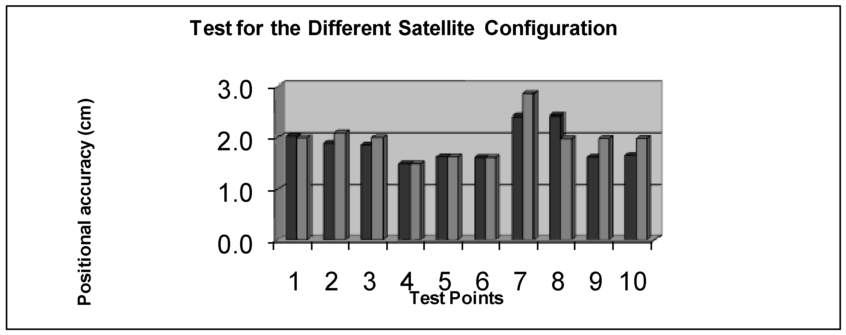
Figure 4.
Positional accuracies for Case 2.
Figure 4.
Positional accuracies for Case 2.
In studying the differences in
Table 2 it can be seen that 2 cm mean difference is obtained for the x and y coordinate components while there is about 3 cm of mean difference in the z-axis direction of, a half order higher than for the plane coordinates. Yet again these differences show that almost the same precisions can be derived from RTK GPS, even with the different satellite configurations.
Similarly, positional accuracies (m
p) for each point are also computed for Case 2 for both observation periods. From
Figure 4 it can be deduced that a pattern similar to the one in case 1 is repeated in case 2, producing very good results in terms of internal accuracies of RTK GPS, even with different satellite configurations.
Case 3: Different Reference Station
The purpose of this test is to observe the change, if any, in accuracy in the case a different reference station is used. For this test two sets of observations were conducted on the same test points, but using a different reference station in each period. In the first period the point 50960, the same reference station as the previous two tests, was chosen as the reference station; as for the second period, the point 50477, which is on the ground and in the vicinity of the test area, but is close to the objects that might obstruct the radio signals, was taken as the reference station. This point 50477 was selected as the reference station because it is not always possible to find a reference station overlooking the object points and having a clear sight of signal transmission during a data collection for most GIS applications.
Table 3.
Differences in coordinate components in Case 3.
Table 3.
Differences in coordinate components in Case 3.
| Coordinate component | Min. Diff. [cm] | Max. Diff. [cm] | Mean [cm] |
|---|
| x-axis | 1.8 | 5.6 | 3.3 |
| y-axis | 0.4 | 7.9 | 3.0 |
| z-axis | 0.7 | 8.5 | 4.2 |
Studying
Table 3, which shows the minimum and maximum differences on each coordinate component and mean values calculated from these differences one may see that meaningful differences are obtained in this test with regards to the previous two tests. The plausible explanation for this discrepancy between the previous two and this test, which is still acceptable for GIS purposes, is that the reference station selected for this test is partially covered by buildings and urban structures. This goes to show that where the reference station is chosen may prove to be significant.
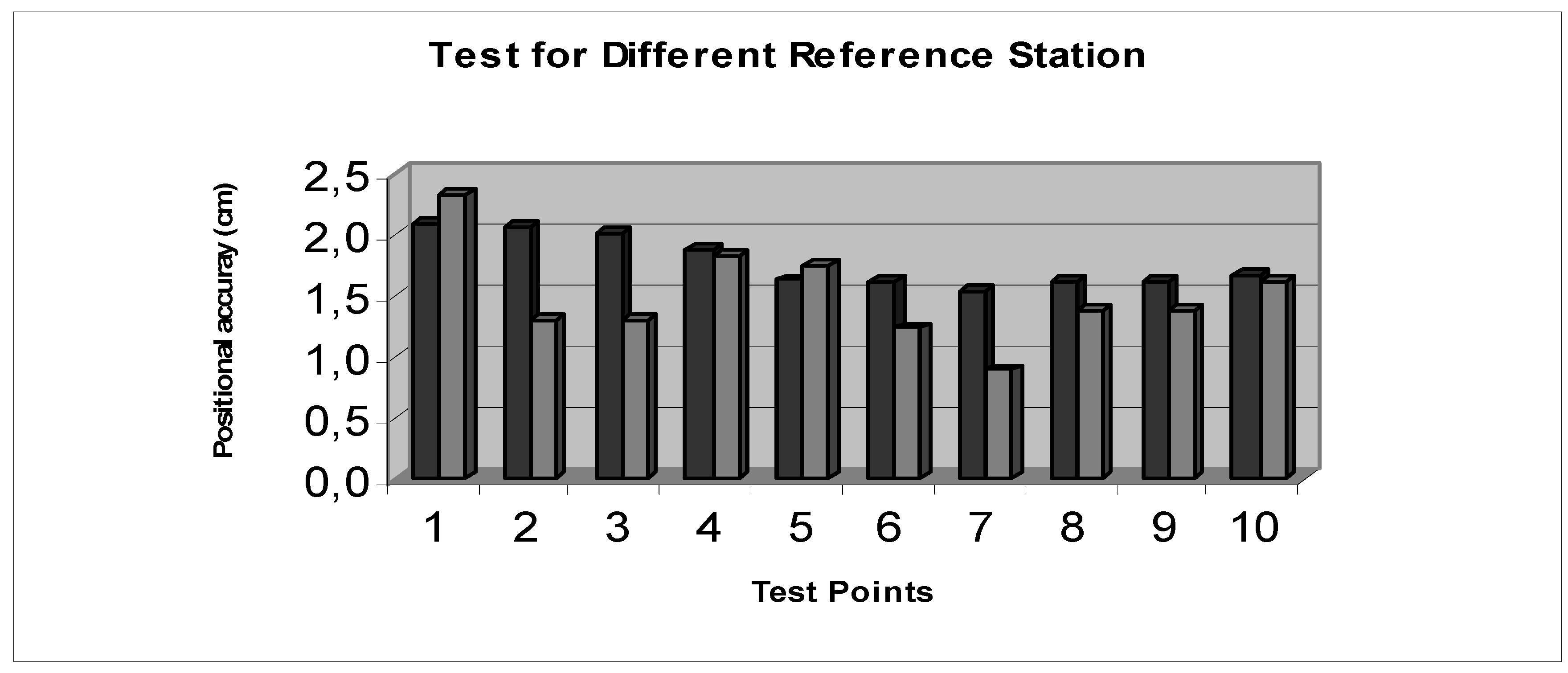
Figure 5.
Positional accuracies for Case 3.
Figure 5.
Positional accuracies for Case 3.
The positional accuracies in
Figure 5 are computed the same way as before and slightly more meaningful differences are present here than in previous tests. Despite the differences between two periods of observations all the positional accuracies remain under about 2 cm, yet again within the similar accuracies yielded by Case 1 and 2.
3.2. Test 2: Observing External Accuracy
Two different testing scenarios, and of course two different test fields, are considered for this test. In the first case, RTK GPS results are compared to the results from static GPS measurements, for the second case they are compared with the results from conventional terrestrial measurements.
Case 1: Static GPS versus RTK GPS
For this test a radial network with six points is taken into consideration in the region of Acemler, a district in the city of Bursa. In this test, for comparison reasons the static GPS method is chosen since in literature it is proven to produce the most accurate positions which can be obtained from GPS measurements.
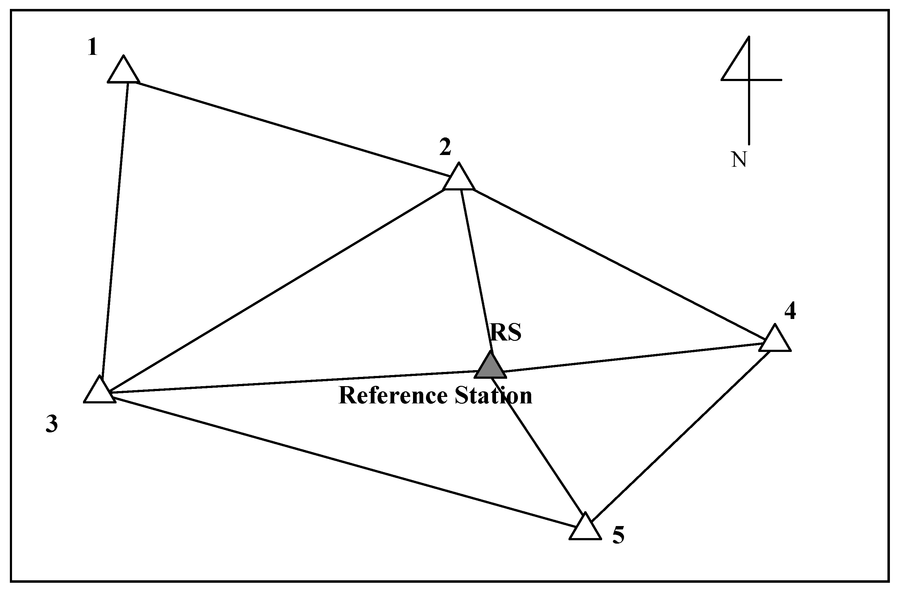
Figure 6 depicts the network configuration used in this test and
Picture 2 shows the test area and test points in a bird’s eye view both in Case 1 and 2. All the points in the network are especially chosen in the densely built-up areas of the city for GIS application purposes, but free from obstructions for radio signals for RTK to be easily used. In both static and RTK GPS observations, the point RS, which is situated on the roof the BUSKI headquarter building, is taken as the reference station. The distances between the reference station and the other points range 1.3 – 2.9 km.
Figure 6.
Configuration of points in the network used in Test 1.
Figure 6.
Configuration of points in the network used in Test 1.
Picture 2.
Bird’s eye view of the Test 2 area (courtesy of Google-Earth).
Picture 2.
Bird’s eye view of the Test 2 area (courtesy of Google-Earth).
The static GPS observations were first carried out in the network with five sessions each comprising 30 minutes of observations made with three Zeiss GePos Experience
TM GPS receivers. The same points were then measured with RTK GPS approach, and the differences between these two approaches are tabulated on the basis of differences in each coordinate axes in
Table 4.
Table 4.
Differences in coordinates between static and RTK GPS positions.
Table 4.
Differences in coordinates between static and RTK GPS positions.
| Points | Distance from ref. station (km) | Differences [cm] |
|---|
| dx | dy | dz |
|---|
| 1 | 2.91 | 4.1 | -4.9 | 5.7 |
| 2 | 1.29 | -1.9 | -0.6 | 8.8 |
| 3 | 1.97 | -0.3 | 0.1 | 1.0 |
| 4 | 1.31 | -0.7 | 2.9 | 7.5 |
| 5 | 1.35 | 6.6 | -2.0 | -3.0 |
Table 5.
Analysis of differences between the static and RTK GPS positions.
Table 5.
Analysis of differences between the static and RTK GPS positions.
| Differences | Min. (cm) | Max. (cm) | Mean (cm) | RMS (cm) |
|---|
| x-axis | 0.3 | 6.6 | 2.7 | 2.35 |
| y-axis | 0.1 | 4.9 | 2.1 | 1.72 |
| z-axis | 1.0 | 8.8 | 5.2 | 2.86 |
A study of how much these differences vary is illustrated in terms of minimum and maximum differences, mean values of these differences and root mean square (rms) values in
Table 5.
As can be seen from
Table 4 and
Table 5, the rms values computed from the positioning differences obtained from this test tend to be below 3 cm. From these results it is obvious that RTK GPS method can produce positions almost as accurate as the static GPS approach, even in densely built-up areas. One should keep in mind that these accuracies are only achievable for baselines shorter than 5 km and where strong data links are available, which is usually the case when collecting data for GIS purposes.
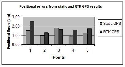
Figure 7.
Positional errors from Static and RTK GPS results
Figure 7.
Positional errors from Static and RTK GPS results
Figure 7 depicts the positional errors (m
p) computed from all coordinates for both methods. Studying the graph, however, shows that the static GPS tends to produce slightly better results than those of RTK GPS method, still under 3 cm level. But, at what cost? Longer occupation times such as half an hour to an hour in static GPS as opposed to seconds in RTK GPS.
Case 2: Conventional Terrestrial Method versus RTK GPS
For this test, eight points from the test field used in all three cases of Test 1 are employed in a close traverse fashion. In first step of this test, a Zeiss Rec Elta 50RS
TM total station is set up on these points of the traverse and observed 93 detail (object) points in the test field. Thus, all these 93 object points are positioned with conventional terrestrial method in local datum frame (ED50). Then, these object points are occupied by RTK GPS for a few seconds and their coordinates are transformed to the local datum system using three of the traverse points whose coordinates are known in both systems. To compare the results obtained from both methods (conventional terrestrial and RTK GPS)
Table 6 is prepared for the minimum and maximum differences on each coordinate component, and mean values and root mean square (rms) values calculated from these differences.
Table 6.
Analysis of differences between RTK GPS and terrestrial positions.
Table 6.
Analysis of differences between RTK GPS and terrestrial positions.
| Coordinate component | Min. Diff. [cm] | Max. Diff. [cm] | Mean [cm] | RMS [cm] |
|---|
| x-axis | 0.2 | 6.0 | 2.6 | 1.71 |
| y-axis | 0.1 | 5.0 | 2.1 | 1.31 |
| z-axis | 0.9 | 9.0 | 3.7 | 2.60 |
From
Table 6 it can be gathered that the accuracy of RTK GPS method is better than 3 cm. This value is comparable with conventional terrestrial methods and manifests that RTK GPS method is an adequate data acquisition method for GIS applications. The following can also be considered as advantages of RTK GPS over conventional terrestrial methods:
Conventional terrestrial methods require interstation visibility, thus depend on other known points in the area.
Positioning 93 points with terrestrial methods takes about 3.5-4 hours while it takes less than an hour with RTK GPS method; thus, less expenditure for field work.
Terrestrial methods require densified points to transfer coordinates to objects points, whereas no need for densification in case of RTK GPS; hence the densification costs.
In RTK GPS only one person is adequate for the task while in terrestrial method it is necessary to employ two or three field personnel; thus the personnel costs.
RTK GPS is an all-weather and 24/7 method whereas terrestrial methods can only be utilized at daytime and dry weather; thus, the planning and working costs.
Obviously every system has shortcomings as well as advantages. Only disadvantage with RTK GPS is that GPS system does not work in places populated by high-rise buildings and tall tree canopies, under bridges and sheltered places. In these cases, the points positioned by RTK GPS can be economically and easily made use as traverse points and give way to using total stations. This kind of integration is still advantageous with respect to the sole terrestrial solution.
4. Conclusions
In order to test the performance of RTK GPS we have carried out two main tests. The first one is to test the internal accuracy of RTK GPS. It is found that with any satellite configuration the required high accuracies are obtainable. In this test we also included to study the effects of different, or rather poor quality, reference station at outlaying positions. Findings are encouraging and in favour of RTK GPS.
The second test was conducted to observe the external accuracy of RTK GPS. For this purpose two different scenarios are accounted for. In the first scenario RTK GPS is put to test in comparison with static GPS and came out with suitable accuracies. Keeping in mind that for the same points static GPS measurements took almost 5 hours, plus the journey times to the points and at least two personnel whereas in RTK GPS the only time taken into account is the journey times to the points! This is because the observation itself only takes a few seconds. In the second scenario we have also tested the performance of RTK GPS against conventional terrestrial method of utilizing a total station for positioning the object points. RTK GPS comes out of this comparison with flying colours. Not only does it achieve the accuracies the conventional terrestrial method could provide but also it does in less time and with less field staff, let alone it is an all-weather and 24/7 working system and does not require interstation visibility.
In all the tests carried out in this study we reached an achievable and repeatable accuracy of approximately 2.5 cm. And this accuracy is considered adequate for any GIS applications that require sub-decimetre accuracies such as in producing cadastre plans, in preparation of large scale plans, in zoning applications, in staking out canal and pipe line projects etc.


