Article

Remotely Sensed Estimation of Net Primary Productivity (NPP) and Its Spatial and Temporal Variations in the Greater Khingan Mountain Region, China

1
School of Geographical Sciences, Northeast Normal University, Changchun 130024, China
2
College of Environmental Science and Engineering, Tongji University, Shanghai 200092, China
3
Jilin Surveying and Planning Institute of Land Resources, Changchun 130061, China
4
Land Consolidation and Rehabilitation Center of Jilin Province, Changchun 130061, China
*
Author to whom correspondence should be addressed.
Sustainability 2017, 9(7), 1213; https://doi.org/10.3390/su9071213
Submission received: 25 March 2017 / Revised: 5 July 2017 / Accepted: 6 July 2017 / Published: 10 July 2017
(This article belongs to the Special Issue Sustainability in the Mountains Region)

Abstract

:
We improved the CASA model based on differences in the types of land use, the values of the maximum light use efficiency, and the calculation methods of solar radiation. Then, the parameters of the model were examined and recombined into 16 cases. We estimated the net primary productivity (NPP) using the NDVI3g dataset, meteorological data, and vegetation classification data from the Greater Khingan Mountain region, China. We assessed the accuracy and temporal-spatial distribution characteristics of NPP in the Greater Khingan Mountain region from 1982 to 2013. Based on a comparison of the results of the 16 cases, we found that different values of maximum light use efficiency affect the estimation more than differences in the fraction of photosynthetically active radiation (FPAR). However, the FPARmax and the constant Tε2 values did not show marked effects. Different schemes were used to assess different model combinations. Models using a combination of parameters established by scholars from China and the United States produced different results and had large errors. These ideas are meaningful references for the estimation of NPP in other regions. The results reveal that the annual average NPP in the Greater Khingan Mountain region was 760 g C/m2·a in 1982–2013 and that the inter-annual fluctuations were not dramatic. The NPP estimation results of the 16 cases exhibit an increasing trend. In terms of the spatial distribution of the changes, the model indicated that the values in 75% of this area seldom or never increased. Prominent growth occurred in the areas of Taipingling, Genhe, and the Oroqen Autonomous Banner. Notably, NPP decreased in the southeastern region of the Greater Khingan Mountains, the Hulunbuir Pasture Land, and Holingol.

1. Introduction

Vegetation is the main component of the terrestrial biosphere, and it plays a critical role in mediating the global carbon balance, mitigating the rise of CO2 concentrations in the atmosphere, and controlling global climate change. Net primary productivity (NPP) refers to the total amount of organic matter produced by photosynthesis per unit area in a unit of time after the deduction of autotrophic respiration and is also known as net primary productive forces. NPP is the basis of material and energy interactions in the ecosystem. This parameter not only quantitatively describes the energy input of the biosphere and the amount of CO2 assimilation, but also reflects the cyclic process of carbon flux in the atmosphere, terrestrial ecosystems, and soil. Moreover, it can be used as the main assessment factor in investigations of the regional carbon flux and the regulation of ecological processes [1].
While NPP cannot be measured directly at regional or global scales, it has become an important tool in the estimation of vegetation productivity using computers and models. Based on different application conditions and input data, scholars around the world have established a number of vegetation productivity estimation models driven by remote sensing data [2,3,4,5]. These achievements provide the basis and methods for further terrestrial ecosystem productivity research.
After nearly half a century, dozens of global models exist for estimating NPP, and they can be divided into statistical models, parameter models, and process models according to the modeling mechanism [2]. The Carnegie-Ames-Stanford Approach (CASA) is a light use efficiency (LUE) process model that fully considers environmental conditions and vegetation characteristics [6,7,8], and it has been widely used in terrestrial ecosystem NPP estimations [7,9,10]. However, the CASA has been rarely applied to the Greater Khingan Mountains, and no studies have discussed the relevant parameter settings. An accurate estimation of light use efficiency is one of the key factors in the simulation of productivity using the CASA model. The model developers believed that, under ideal conditions, vegetation exhibits a maximum light use efficiency and set this monthly value to 0.389 g C/MJ [6,8] for all vegetation types. Running et al. [11] assigned the maximum light use efficiency according to the photosynthetic characteristics of different vegetation types when estimating the global terrestrial NPP. Li et al. [12] estimated the monthly NPP of Shenzhen using the MODIS-derived normalized difference vegetation index (NDVI) data and explored the effects of extreme weather on NPP. Li modified the fraction of photosynthetically active radiation (FPAR) model according to the NASA-MOD15 algorithm [13] and the characteristics of vegetation in Shenzhen. Zhu et al. [14] introduced the vegetation classification accuracy into simulations of the maximum light use efficiency of typical vegetation in China. Their result is between the values calculated in the Potter and Running studies. In addition, Zhu estimated the NPP of terrestrial ecosystem vegetation in China by modifying the FPAR model using the relationships among FPAR, NDVI, and the simple ratio (SR). Questions regarding whether the modification of these parameters based on different objects and scales is applicable to NPP estimation in mid-latitude mountain ecosystems and how to select these parameters in future estimations should be discussed. In fact, significant differences in light use efficiency exist among different vegetation types [15], and because light use efficiency is notably affected by temperature, moisture, soil, and individual plant growth, treating it as a constant for all regions on Earth will produce considerable error. Above all, it is necessary to amend the parameters before applying the model to other regions.
Scholars in China who pay attention to the NPP of the mountain system almost always use the ecological process model or MODIS data, and they do little research on mid-latitude mountains [16,17,18]. As for other mountains in the same latitude around the world, most of researchers value the NPP by monitoring the growth of plants [19].
This study focuses on different types of land use, the values of the maximum light use efficiency, calculation methods for solar radiation, combined cases, and the modification of parameters. Taking the Greater Khingan Mountain region as an example and combining a time series of remote sensing data, we use the CASA to improve the NPP estimation model for mountain ecosystems. The goal is to improve the NPP estimation accuracy for mountain ecosystems and provide a basis for the estimation of carbon sources and sinks in a mountain forest ecosystem.

2. Materials and Methods
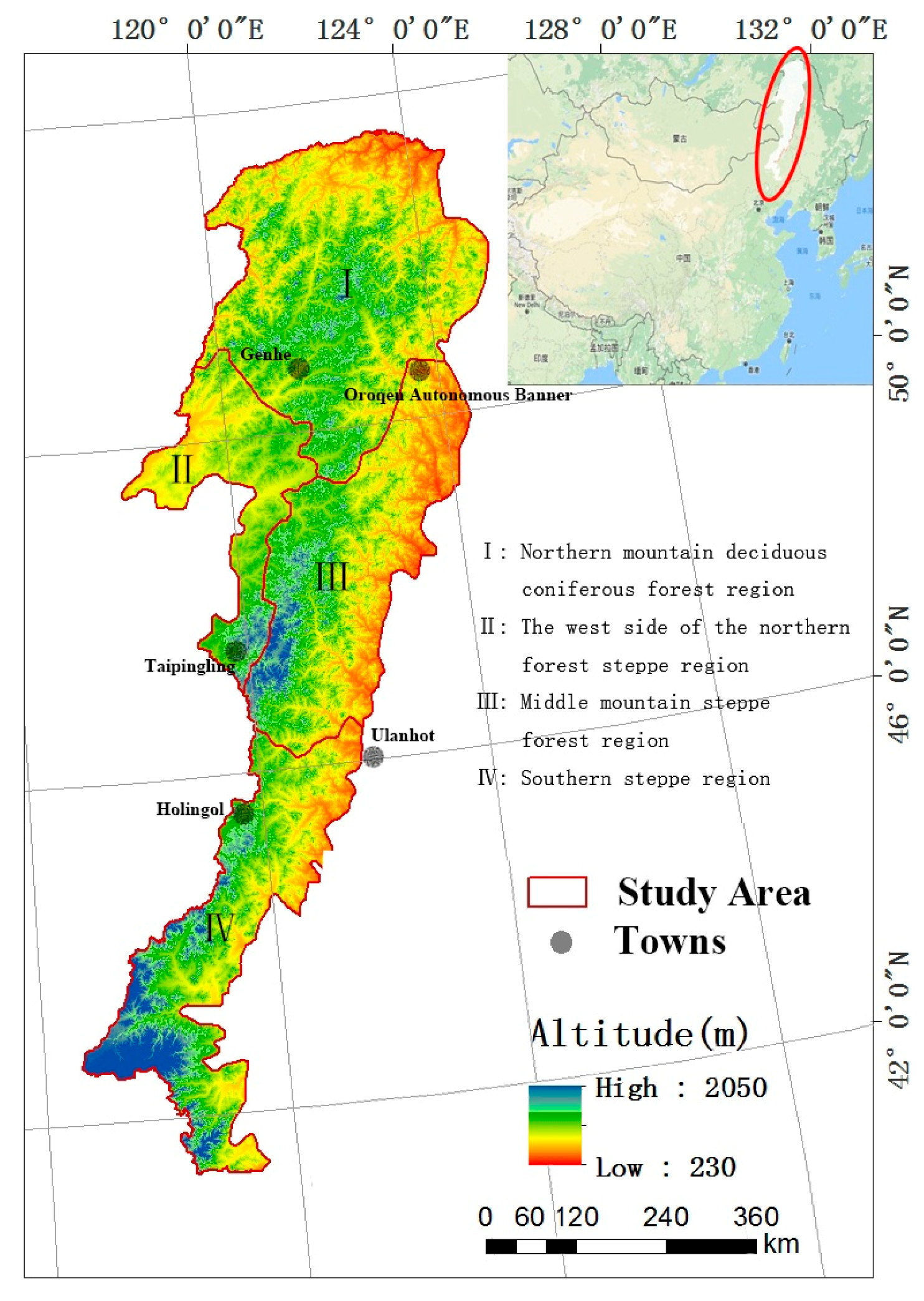
2.1. Study Area

The Greater Khingan Mountain region (40°52′–53°33′ N, 116°25′–125°42′ E) is located in the northernmost region of China, one of the most sensitive areas to global climate change [20,21]. Estimating the net productivity of vegetation in this region is helpful in understanding the carbon sequestration capacity of the forest system in this area and understanding the climate change response mechanism. Thus, we can better predict the future trend of vegetation productivity and its impact on the carbon cycle, as it can be a reference for ecological compensation policy and sustainable forest development. For these reasons, we chose the Greater Khingan Mountain region as the study area and estimated the NPP with the purpose of verifying the applicability and accuracy of this model. The boundary of the Greater Khingan Mountain is defined by the eco-geographical region map of China [22], which divides the Greater Khingan Mountain region into four ecological regions: (I) the northern deciduous coniferous forest region; (II) the western side of the northern forest steppe region; (III) the middle steppe forest region; and (IV) the southern steppe region (Figure 1).

2.2. Methodology

2.2.1. CASA Model

The CASA is one of the process models for the NPP estimation that uses remote sensing data, and it reflects the influence of natural factors, such as temperature, precipitation, and radiation, on NPP. The specific calculation method and parameter settings are described in Section 3.

2.2.2. Statistical Analysis Method

The data of all the models calculated in this paper are verified with the data obtained from the ground survey via linear correlation analysis.

2.2.3. Trend Analysis Method

The spatial trends of NPP in each pixel were analyzed using the slope of the linear regression equation. The formula is as follows:
a = ( n × j = 1 n j × NPPj ¯ j = 1 n j j = 1 n NPPj ) / [ n × j = 1 n j 2 ( j = 1 n j ) 2 ]
where a represents the inter-annual variation trend for NPP in the Greater Khingan Mountain; n is the time series; and NPPj ¯ represents the NPP value in the jth year. When a > 0, NPP exhibits an increasing trend; when a < 0, it exhibits a decreasing trend.

2.3. Data

2.3.1. GIMMS Dataset

The NDVI data in this paper is the third generation NOAA/AVHRR NDVI data from the Global Inventory Modelling and Mapping Studies (http://ecocast.arc.nasa.gov/data/pub/gimms/3g.v0/, GIMMS NDVI3g). This version of the Global Vegetation Index, released by the National Aeronautics and Space Administration (NASA), provides higher quality data for phenological research at high latitudes. The dataset in this study is in the ENVI standard format, the projection is ALBERS, the time resolution is 15d, the spatial resolution is 8 km, and the time span is from January 1982 to December 2013.
The dataset has been preprocessed with radiation correction, geometric correction, and image enhancement, and the monthly maximum value of NDVI was obtained by the maximum value composite (MVC), which reduces the effects caused by the atmosphere, sensor angle, and solar height angle.

2.3.2. Meteorological Data

The meteorological dataset is derived from data recorded at 97 meteorological stations between 1982 and 2013.
In this paper, the solar radiation data for each site were calculated using the climatic empirical model. According to the geographical coordinates of each site in the dataset, solar radiation, monthly average temperature, and precipitation data were interpolated into a raster dataset using the ordinary kriging method at a spatial resolution of 8 km to match the GIMMS NDVI3g data.

2.3.3. Vegetation Type Dataset

The vegetation type data were obtained from China’s 1:1,000,000 vegetation dataset. However, the differences in vegetation types used by different researchers were considered when setting values for SR, NDVI, and εmax. The comparison with the original vegetation types can be found in the following discussion.

2.3.4. Field Data

More than 4000 forest inventory data points for five forest types (larch, birch, pine, spruce, and aspen) were collected, including the quadrat location, quadrat area, volume, tree species, stand age, and diameter at breast height. The NPP was estimated using Equation (2) [23]:
N PP = B aA + bB
where NPP is in units of Mg ha−1 yr−1 and A is the stand age (year); a and b are constants for a specific forest type. B represents the stand biomass (Mg ha−1) and was calculated using Equation (3) [24]:
B = V c + dV
where B and V are the stand biomass (Mg ha−1) and stand volume (m3/ha), respectively, and c and d are constants based on the specific forest type.
Finally, the mean NPP data in 8 km pixels are calculated to match the remote sensing data.

3. NPP Estimation

3.1. General Framework

The basic principle of the CASA model is that a linear relationship exists between the net primary productivity and the absorbed photosynthetically active radiation (APAR) and actual light use efficiency (ε):
NPP ( x , t ) = APAR ( x , t ) × ε ( x , t )
where APAR(x, t) represents the photosynthetically active radiation absorbed by pixel x in month t, and ε(x, t) represents the actual light use efficiency of cell x in month t; the unit for both terms is g C/MJ.
The APAR of plants depends on the total solar radiation and the FPAR of photosynthetically active radiation (PAR) and can be described using Equation (5):
APAR ( x , t ) = SOL ( x , t ) × FPAR ( x , t ) × 0.5
where SOL(x, t) is the total solar radiation (unit: MJ/m2) at pixel x in month t; FPAR(x, t) is the ratio of photosynthetically active radiation absorbed by the vegetation layer (unitless); and 0.5 represents the ratio of solar active radiation to total solar radiation that can be used by vegetation.
Potter considered that a maximum light use efficiency exists for plants under ideal conditions and that the maximum light use efficiency under actual conditions is mainly affected by temperature and moisture. This relationship can be expressed using Equation (6):
ε   ( x , t ) = T ε 1 ( x , t ) × T ε 2 ( x , t ) × W ε ( x , t ) × ε max
where Tε1(x, t) and Tε2(x, t) denote the effect of temperature stress (unitless), Wε(x, t) denotes the effect of water stress (unitless), and εmax is the maximum light use efficiency under ideal conditions (Unit: g C/MJ).
By combining Equations (5) and (6), we obtain Equation (7):
NPP ( x , t ) = SOL ( x , t ) × FPAR ( x , t ) × 0.5 × T ε 1 ( x , t ) × T ε 2 ( x , t ) × W ε ( x , t ) × ε max

3.2. SOL Algorithm

Taking the basic time scale of this study into account, the monthly total solar radiation can be calculated using the daily solar radiation. The daily total solar radiation can be determined via Equation (8):
S 0 = TI 0 π ρ 2 × ( ω 0 sin ( φ ) sin ( δ ) + cos ( φ ) cos ( δ ) sin ( ω 0 ) )
where S0 is the atmospheric external solar radiation (unit: MJ/m2·d); T is the period; I0 is the solar constant; φ is the geographical latitude; and ρ , ω0, and δ are the relative distance between the sun and the Earth, the solar hour angle, and the solar declination as calculated by Equations (9)–(11), respectively:
ρ = Sqrt { 1 / [ 1 + 0.033 × cos ( 2 π J / 365 ) ] }
where J represents the day of the year.
ω 0 = arcos ( tan φ tan δ )
δ = 0.409 × sin ( 0.0172 J 1.39 )  
The daily total solar radiation can be calculated using the relationship between the solar radiation and sunshine percentage, as shown in Equation (12):
SOL d = ( a + b × n N ) × S 0
where SOLd is the daily total solar radiation (unit: MJ/m2·d), n is the actual sunshine duration, N is the maximum sunshine duration, the units are hours, and the ratio is the sunshine percentage. The terms a and b are two constants and, according to previous research experience and the situation of the study area, are assigned values of 0.207 and 0.725, respectively [25].

3.3. FPAR Algorithm

In this paper, we discuss three kinds of FPAR models using NDVI in the calculations.
1. FPAR model proposed by Tianhong Li [12].
This model is based on the relationship between NDVI and FPAR provided by the NASA-MOD15 algorithm.
FPAR = { 0 NDVI 0.075 1.054 * NDVI 0.036 0.075 < NDVI < 0.875 0.916 NDVI 0.875
2. FPAR model proposed by Zhu [26].
This model is based on the research of Sellers.
FPAR ( x , t ) = ( NDVI ( x , t ) NDVI i , min ) × ( FPAR max FPAR min ) ( NDVI i , max NDVI i , min ) + FPAR min ,
where NDVIi,max and NDVIi,min correspond to the NDVI maximum and minimum values of the i-th vegetation type, respectively.
In this model, the accuracy of the vegetation classification is introduced, and the errors caused by noise in a remote sensing image are eliminated by using the lower quantile. The combined vegetation types, used by both Zhu and this paper, and the maximum and minimum NDVI and SR, are listed in Table 1.
Other research shows [27] that there is a remarkably linear relationship between FPAR and SR, as shown in Equation (15).
FPAR ( x , t ) = ( SR ( x , t ) SR i , min ) × ( FPAR max FPAR min ) ( SR i , max SR i , min ) + FPAR min
where SR(x,t) can be calculated via Equation (16) and SRi,max and SRi,min represent the 95% and 5% lower quantiles of i-th vegetation NDVI, respectively.
SR ( x , t ) = 1 + NDVI ( x , t ) 1 NDVI ( x , t )
These two methods are combined and the average is taken as an estimate of the FPAR (Equation (17)).
FPAR ( x ,   t ) = α FPAR NDVI + ( 1 α ) FPAR SR
where FPARNDVI is the result of Equation (14), FPARSR is the result of Equation (15), and α is a constant with a value of 0.5.
According to the results of previous studies and field survey data [28], the range of FPAR should be between 0 and 1, but since the range of FPARSR in the model cannot be found in the literature, the maximum of FPARSR can be determined as follows. One methods involves setting the value to 0.95 according to the FPARSR model proposed by Potter (Equation (18)). Another method involves setting it to 0.90255, which is the result of putting 0.95 into Equation (12), i.e., the combined Potter and Los model.
3. FPAR model proposed by Potter.
Potter chose the NDVI and vegetation type to represent the FPAR with a maximum of no more than 0.95, as shown in Equation (18).
FPAR ( x , t ) = min [ SR ( x , t ) SR i , min SR i , max SR i , min   , 0.95 ]
where SR(x, t) is the result of Equation (16); SRi,min is the SR value of bare land, with an assigned value of 1.08; and SRi,max is related to the vegetation type and ranges between 4.14 and 6.17. The SRmax values of vegetation according to the research of Seller are listed in Table 2.

3.4. Algorithm of Tε1, Tε2 and Wε

The terms Tε1 and Tε2 represent the temperature stress of plant photosynthesis and can be determined using Equations (19) and (20), respectively.
T ε 1 ( x ,   t ) = 0.8 + 0.02 × T opt ( x )   0.0005 × [ T opt ( x ) ] 2
T ε 2 = C / { 1 + exp [ 0.2 × ( T opt 10 T ) ] } / { 1 + exp [ 0.3 × ( T opt 10 + T ) ] }
where Topt(x) is the monthly average temperature for a region when the NDVI value is the highest; C is a constant (here, the values of 1.1814 and 1.1919, proposed by Potter and Tianhong Li, respectively, are used for comparison); T is the average monthly temperature; and W represents the moisture stress of plant photosynthesis and ranges from 0.5 to 1:
W ε ( x ,   t ) = 0.5 + 0.5 × E ( x ,   t ) / E p ( x ,   t )
where E(x, t) is the regional actual evapotranspiration (unit: mm), which can be calculated according to the regional real evapotranspiration model established by Zhou and Zhang [29] (Equation (22)), and Ep(x, t) is the area potential evapotranspiration (unit: mm), which can be calculated according to Boucher’s complementary formula (Equation (24)).
E ( x , t ) = { P ( x ,   t ) × R n ( x ,   t ) × [ P 2 ( x ,   t ) +   R n 2 ( x ,   t ) + P ( x ,   t ) × R n ( x ,   t ) ] } / { [ P ( x ,   t ) + R n ( x ,   t ) ] × [ P 2 ( x ,   t ) + R n 2 ( x ,   t ) ] }
where E(x, t) is the net amount of surface radiation (unit: MJ/m2) of the pixel x in month t, and P(x, t) is the precipitation in pixel x in t month (unit: mm), which can be obtained by the empirical formula established by Guangsheng Zhou and Xinshi Zhang (Equation (23)).
R n ( x , t ) = [ E p 0 ( x ,   t ) × P ( x , t ) ] 0.5 × { 0.369 + 0.598 × [ E p 0 ( x ,   t ) / P ( x , t ) ] 0.5 }
E p ( x ,   t ) = [ E ( x ,   t ) + E p 0 ( x ,   t ) ] / 2
where Ep0(x,t) is the potential evapotranspiration in an area (unit: mm), which can be calculated using the vegetation-climate model proposed by Thornthwaite (Equations (25)–(27)).
E p 0 ( x ,   t ) = 16 × [ 10 × T (   x , t ) / I ( x ) ] a ( x )
a ( x ) = [ 0.6751 × I 3 ( x )   77.1   × I 2 ( x ) + 17920 × I ( x ) + 492390 ] × 10 6
I ( x ) = i = 1 12 [ T ( x , t ) 5 ] 1.514
where I(x) is the heat index from the sum of 12 months, and a(x) is a constant that differs depending on the location.

3.5. The Maximum Light Use Efficiency

The monthly maximum light use efficiency has a great influence on the NPP estimation result, and it varies with the vegetation type. In this paper, we compare the results of Zhu [15] and Running [11]. The vegetation types and their corresponding εmax values are listed in Table 3.

3.6. Model Implementation

According to the above discussion, the four parameters of FPAR, FPARmax, Tε2, and εmax have different values and calculation methods. To find a more suitable method, all possible values of these four parameters are permutated and combined. We used Equation (7) and set the name of the parameter creator as a code to form 16 kinds of cases, each of which is listed in Table 4.

4. Results and Discussion

4.1. Precision Verification and Evaluation

4.1.1. Comparison with Field NPP

In this paper, cases 2 and 4 show the strongest correlations with the ground measured data, while cases 5 and 7 show the weakest correlations (Table 5).
Changes in εmax lead to the most significant effects on the result, and the correlations of all models can be divided into two categories based on this parameter. The models using the εmax of Running are more strongly related to the field data than those using the εmax of Zhu. The following influential factors are FPAR and FPARmax, and they present varying levels of importance in these two categories. Obviously, the FPAR model proposed by Li is the best one in all the cases. Then, the next best combination is the εmax of Running and the FPAR of Zhu, or the εmax of Zhu and the FPAR of Potter. Though the FPAR of Li is based on plants in Shenzhen, the vegetation coverage and productivity of the plants in the Greater Khingan Mountain region are also very high during the growing season. Thus, the carbon capacity of the plant species is more significant than the overall vegetation type. Consequently, the FPARmax should be 0.916. In contrast, when using the FPAR of Zhu, the FPARmax should be 0.90255. Tε2 has little or no impact on the NPP estimation.

4.1.2. Comparison with Other Researchers Who Used the Same Model

Table 6 shows that the estimation results in this paper are similar to those of other scholars when using the same model. Cases 5, 7, 9, 13, and 15 are close to the minima obtained in other studies, whereas cases 2 and 4 are close to the maxima obtained in other studies. Moreover, cases 14 and 16 are close to the average of field data.

4.1.3. Accuracy Evaluation Summary
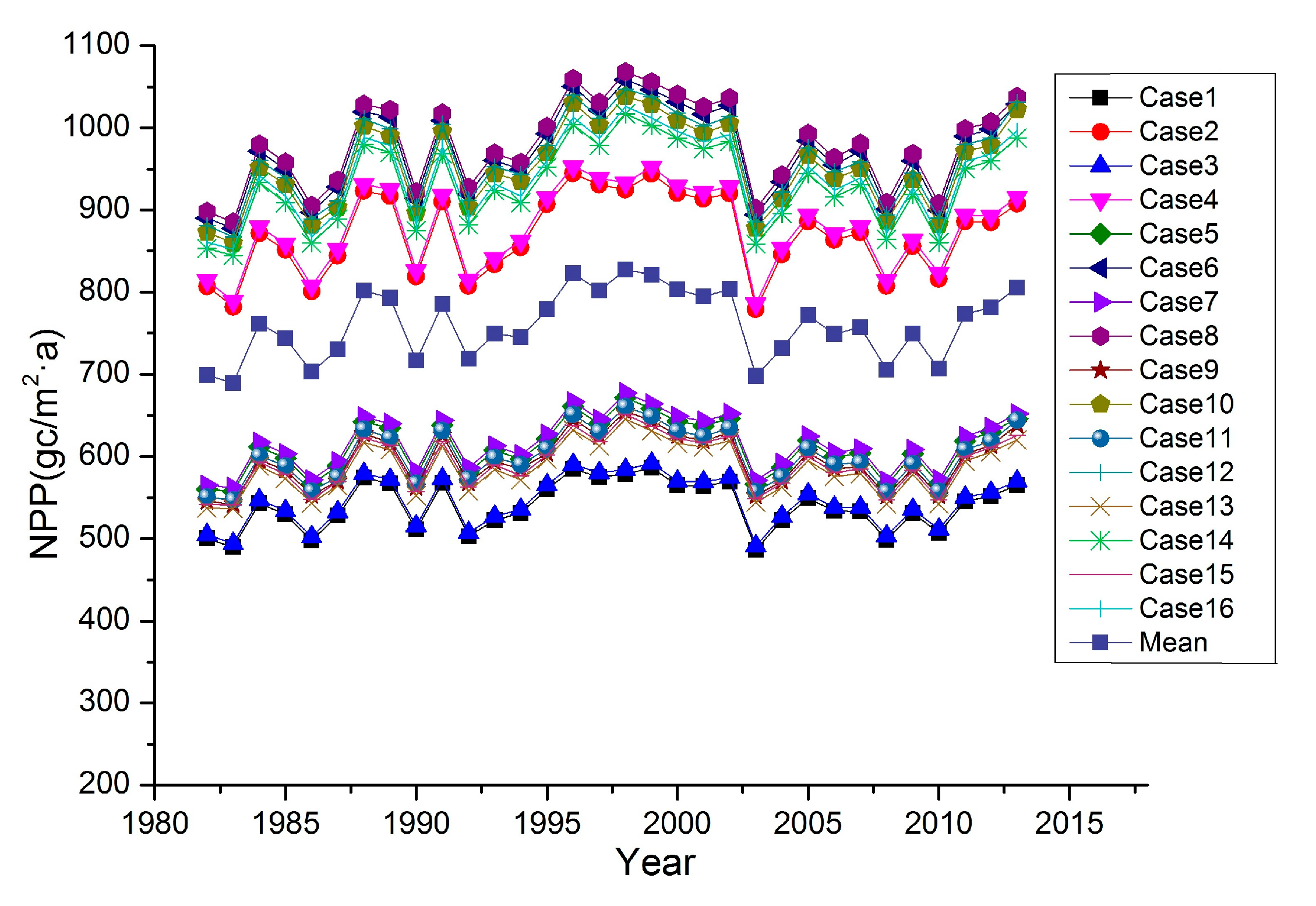
Based on the above two methods of accuracy evaluation for the Greater Khingan Mountain region, the selection of εmax has the greatest impact on the estimation results, followed by FPAR and FPARmax, whereas Tε2 does not show a significant effect. Obviously, the FPAR model proposed by Li is the best one in all the cases. The next best combination is the εmax of Running and the FPAR of Zhu or the εmax of Zhu and the FPAR of Potter. The FPARmax should be 0.916. However, when using the FPAR of Zhu, the FPARmax should be 0.90255. All the results are similar to those of previous studies and the observed values.

4.2. Trend of NPP

The overall level of NPP in the Greater Khingan Mountain region increased during the 32-year study period. The highest NPP values occurred from 1994–2001, when the rain and heat conditions were conducive to vegetation growth. Extreme low values in 1983 and 2003 may be associated with extreme weather conditions. The Greater Khingan Mountain region experienced low temperatures and rainy weather in 1983 and high temperatures and drought in 2003. Both extreme weather conditions were highly detrimental to plant photosynthesis. In addition, two dips in approximately 1990 and 2003 are present in Figure 2. The former may be related to the double impacts of precipitation and the Greater Khingan Mountain “5 6 large fire” that occurred in 1987. Some studies [30] have shown that the severe fires slowed NPP growth to a certain extent and that the forest then gradually recovered. The study area selected in this paper is much larger than the fire area; thus, the comprehensive results are consistent with the simulations. The dip in 2003 was due to the continuous decline in precipitation leading to successive years of drought starting in 2002.

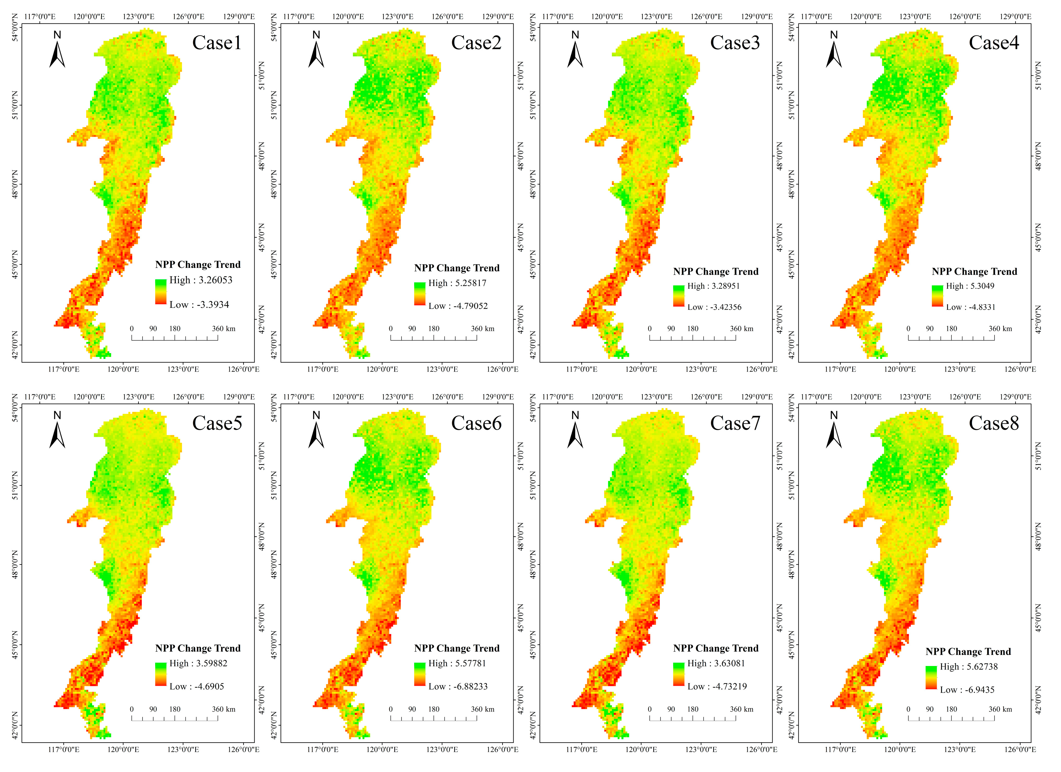
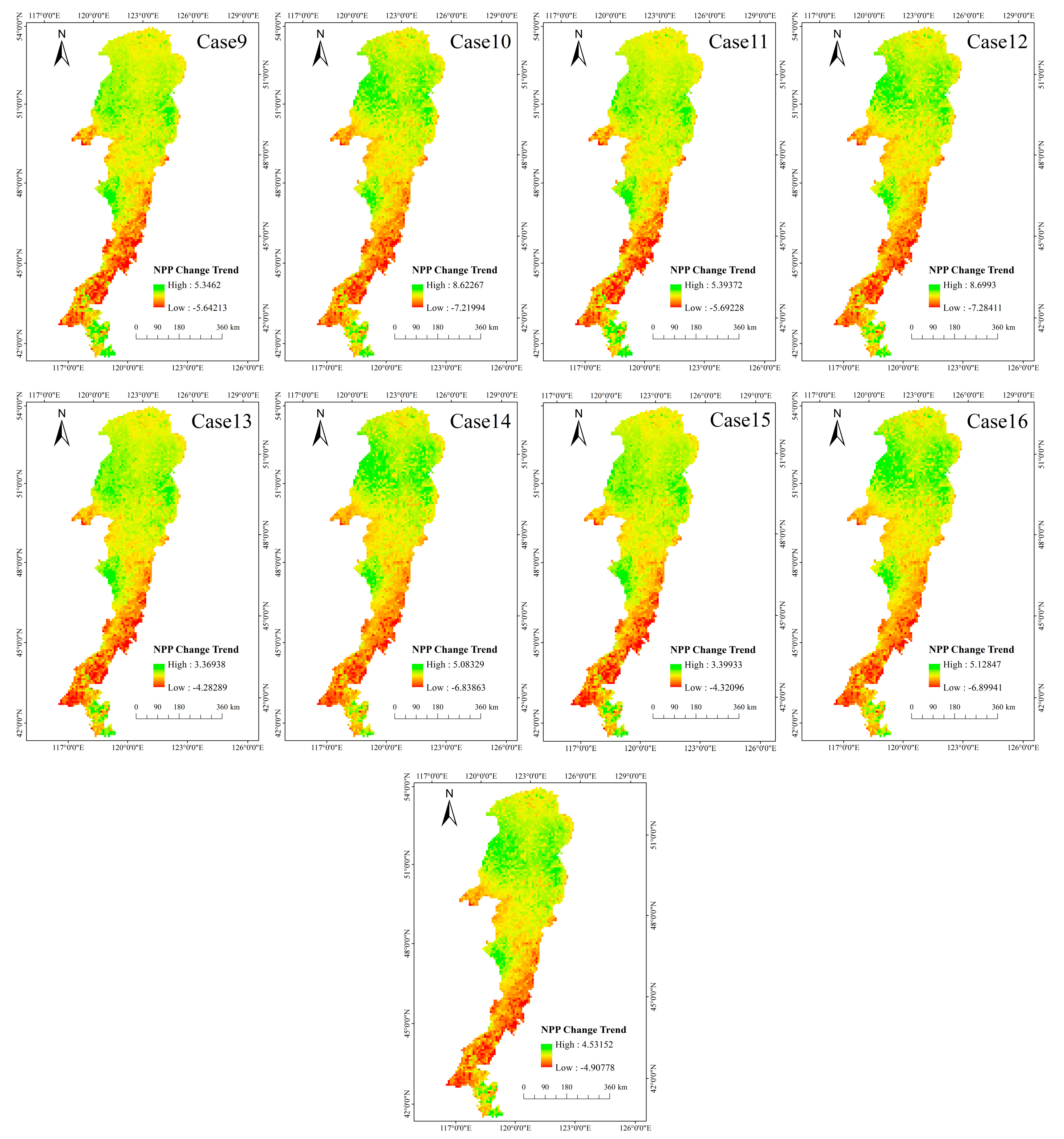
4.3. Spatial Patterns of NPP Trends

As seen from Figure 3, the area with decreasing NPP is significantly smaller than the areas with constant or increasing NPP. Three main distributions of the decreasing trend exist. The first one is the southeastern part of the Greater Khingan Mountains, which is located at the juncture of the Inner Mongolia Plateau and the Northeast Plains, west of the Hunshandake Sandy Land and east of the Kerqin Sandy Land. The forest coverage is low, and the ecological environment is poor. Additionally, urban areas are concentrated in this region, and destruction due to urbanization can also lead to a reduced NPP. The second one is the Hulunbuir Pasture Land, where desertification, transition grazing, and reclamation activities have led to a decrease in NPP in this region. The third one is near the city of Holingol. This city is a new industrial city in the hinterland of the Kerqin grassland. The fragility of grassland vegetation and the destruction of the ecological environment by mining development may be the main reasons for the decrease in NPP in this area.
We divided the values into several levels: pixels with values less than 0 represented areas in which NPP decreased; pixels with values between 0 and 2 represented areas with little change in NPP; and pixels with values greater than 2 represented areas in which the NPP increased (Table 7).
Increasing trends are also distributed in three areas, namely Genhe, the Oroqen Autonomous Banner, and Taipingling. These three sites are located in the foothills of the Greater Khingan Mountain region and feature river irrigation. There are inherent advantages to improving the forest cover by either artificial or natural means. Moreover, in recent years, these three cities have focused on ecological and environmental protection, which is also a force of NPP growth.
The ecological status of the Greater Khingan Mountain region was good. From 1982 to 2013, the NPP decreased in 14.77% of the study area, remained unchanged in more than half of the study area, and increased in 9.27% of the study area.

5. Conclusions

In this study, we estimated the NPP values of different vegetation in the Greater Khingan Mountain region from 1982 to 2013 using GIMMS3g data and 16 cases based on the CASA model with various parameters. By comparing our results with observed NPP data and results from other Chinese researchers, we reached the following conclusions. The selection of maximum light use efficiency, followed by FPAR and FPARmax, has the greatest impact on the estimation results, while Tε2 shows no significant effect on the estimation results. When applying the CASA model to other similar regions, the recommended parameter settings include the εmax of Running and the FPAR of Li. When using the FPAR model of Zhu, the best FPARmax value is 0.90255. Similar temporal and spatial variations in the NPP in the Greater Khingan Mountain region are presented by all cases in this paper, and the overall NPP level in the Greater Khingan Mountain region increased over the 32-year study period. The northern Greater Khingan Mountain region, especially in Genhe, the Oroqen Autonomous Banner, and Taipingling, exhibits an increasing NPP trend. The southeastern Greater Khingan Mountains, Hulunbuir Pasture Land, and Holingol are characterized by decreasing NPP. The NPP in other areas remained unchanged.
When applying the CASA model in other mountain areas, we should pay attention to the following aspects. Firstly, the εmax is more influenced by the carbon capacity of plant species than by the overall type of vegetation. Secondly, existing studies on NPP have emphasized the effects of temperature- and water-induced stress on FPAR, which vary by location. However, the key information provided by remote sensing models is the radiance and reflectance of plants. Therefore, we have to build better FPAR models to improve the accuracy of the estimation. Finally, we need field observation values from areas corresponding to remote sensing images in order to obtain higher-accuracy results.

Acknowledgments

The authors would like to thank the entire Global Inventory Modeling and Mapping Studies (GIMMS) group for permitting the use of the NDVI3g dataset. This work was supported by the National Natural Science Foundation of China (Grant No. 41501449), the National Key Research and Development Project (Grant No. 2016YFA0602301), the Fundamental Research Funds for the Central Universities (Grant No. 2412017FZ021), and the National Natural Science Foundation of China (Grant Nos. 41571489, 41601438, 41571078, 41630749 and 41571405).

Author Contributions

Qiang Zhu contributed to the geospatial data analysis and the writing of the manuscript. Jianjun Zhao took the lead on the design, the assessment, and the writing of the paper. Zhenhua Zhu, Zhengxiang Zhang, Hongyan Zhang, and Xiaoyi Guo contributed analysis tools and reviewed the manuscript. Yunzhi Bi and Li Sun were responsible for the collection of data. All authors have read and approved the final manuscript.

Conflicts of Interest

The authors declare no conflict of interest.

References

  1. Field, C.B.; Behrenfeld, M.J.; Randerson, J.T.; Falkowski, P. Primary production of the biosphere: Integrating terrestrial and oceanic components. Science 1998, 281, 237–240. [Google Scholar] [CrossRef] [PubMed]
  2. Ruimy, A.; Saugier, B.; Dedieu, G. Methodology for the estimation of terrestrial net primary production from remotely sensed data. J. Geophys. Res. Atmos. 1994, 99, 5263–5283. [Google Scholar] [CrossRef]
  3. Nemani, R.R.; Keeling, C.D.; Hashimoto, H.; Jolly, W.M.; Piper, S.C.; Tucker, C.J.; Myneni, R.B.; Running, S.W. Climate-driven increases in global terrestrial net primary production from 1982 to 1999. Science 2003, 300, 1560–1563. [Google Scholar] [CrossRef] [PubMed]
  4. Peng, S.; Guo, Z.; Wang, B. Use of GIS and RS to estimate the light utilization efficiency of the vegetation in Guangdong, China. Acta Ecol. Sin. 2000, 20, 903–909. [Google Scholar]
  5. Ricotta, C.; Avena, G.; Palma, A.D. Mapping and monitoring net primary productivity with AVHRR NDVI time-series: statistical equivalence of cumulative vegetation indices. Isprs. J. Photogramm. Remote Sens. 1994, 54, 325–331. [Google Scholar] [CrossRef]
  6. Field, C.B.; Randerson, J.T.; Malmström, C.M. Global net primary production: Combining ecology and remote sensing. Remote Sens. Environ. 1995, 51, 74–88. [Google Scholar] [CrossRef]
  7. Piao, S.L.; Fang, J.Y.; Guo, Q.H. Application of CASA model to the estimation of Chinese terrestrial net primary productivity. Acta Phytoecol. Sin. 2001, 25, 603–608. [Google Scholar]
  8. Potter, C.S.; Randerson, J.T.; Field, C.B.; Matson, P.A.; Vitousek, P.M.; Mooney, H.A.; Klooster, S.A. Terrestrial ecosystem production: A process model based on global satellite and surface data. Glob. Biogeochem. Cycles 1993, 7, 811–841. [Google Scholar] [CrossRef]
  9. Chen, L.J.; Liu, G.H.; Li, H.G. Estimating Net Primary Productivity of Terrestrial Vegetation in China Using Remote Sensing. J. Remote Sens. 2002, 6, 129–135. [Google Scholar]
  10. Fang, J.; Piao, S.; Field, C.B.; Pan, Y.; Guo, Q.; Zhou, L.; Peng, C.; Tao, S. Increasing net primary production in China from 1982 to 1999. Front. Ecol. Environ. 2003, 1, 293–297. [Google Scholar] [CrossRef]
  11. Running, S.W.; Thornton, P.E.; Nemani, R.; Glassy, J.M. Global Terrestrial Gross and Net Primary Productivity from the Earth Observing System. In Methods in Ecosystem Science; Springer: New York, NY, USA, 2000; pp. 44–57. [Google Scholar]
  12. Li, T.; Wang, Z. Estimation of Monthly Net Primary Productivity and Its Variation Characteristics in Shenzhen Based on CASA Model, GIS and RS. J. Basic Sci. Eng. 2012, 20, 126–135. [Google Scholar]
  13. Myneni, R.B.; Knyazikhin, Y.; Zhang, Y.; Tian, Y.; Wang, Y.; Lotsch, A.; Privette, J.L.; Morisette, J.T.; Running, S.W.; Nemani, R. MODIS Leafarea Index (LAI) and Fraction of Photosynthetically Activeradiation Absorbed by Vegetation (FPAR) Product (MOD15) Algorithm Theoretical Bas Is Document. Available online: https://modis.gsfc.nasa.gov/data/atbd/atbd_mod15.pdf (accessed on 1 May 2017).
  14. Zhu, W.; Pan, Y.; He, H.; Yu, D.; Hu, H. Simulation of Maximum Light Use Efficiency of Typical Vegetation in China. Chin. Sci. Bull. 2006, 51, 457–463. [Google Scholar] [CrossRef]
  15. Zhu, W. Estimation of Light Utilization Efficiency of Vegetation in China Based on GIS and RS. Geomat. Inf. Sci. Wuhan Univ. 2004, 29, 694–698. [Google Scholar]
  16. Zhang, N.; Yu, G.; Yu, Z.; Zhao, S. Analysis on factors affecting net primary productivity distribution in Changbai Mountain based on process model for landscape scale. Chin. J. Appl. Ecol. 2003, 14, 659. [Google Scholar]
  17. Zhang, J.; Gao, Z.; Gao, W.; Pan, X.; Zhao, S.; Shi, Q.; Lu, G. Landscape heterogeneity and net primary productivity (NPP) of mountain-oasis-desert ecosystems in western China. Proc. SPIE 2004, 5153. [Google Scholar] [CrossRef]
  18. Wang, Q.; Zhang, T.; Yi, G.; Chen, T.; Bie, X.; He, Y. Tempo-spatial variations and driving factors analysis of net primary productivity in the Hengduan mountain area from 2004 to 2014. Acta Ecol. Sin. 2017, 37, 3084–3095. [Google Scholar] [CrossRef]
  19. Stenzel, J.A. Towards Intra-Seasonal Estimation of Forest Net Primary Productivity: Evaluating Automated Dendrometers for High-Temporal Resolution Woody Growth Signals. Ph.D. Thesis, University of Idaho, Moscow, ID, USA, 2016. [Google Scholar]
  20. WU, S.; Pan, T.; Liu, Y.; Deng, H.; Jiao, K.; Lu, Q.; Feng, A.; Yue, X.; Yin, Y.; Zhao, D. Comprehensive climate change risk regionalization of China. Acta Geogr. Sin. 2017, 72. [Google Scholar] [CrossRef]
  21. Hao, C.; Zhao, T. Comparative Research on Regional Respond to Global Climate Change in China. Areal Res. Dev. 2011, 3, 56–61. [Google Scholar]
  22. Zheng, D. China’s Eco-Geographical Region Map; The Commercial Press: Beijing, China, 2008. [Google Scholar]
  23. Zhao, M.; Zhou, G.S. Estimation of biomass and net primary productivity in major planted forests in China based on forest inventory data. For. Ecol. Manag. 2005, 207, 295–313. [Google Scholar] [CrossRef]
  24. Zhou, G.; Wang, Y.; Jiang, Y.; Yang, Z. Estimating biomass and net primary production from forest inventory data: a case study of China’s Larix forests. For. Ecol. Manag. 2002, 169, 149–157. [Google Scholar] [CrossRef]
  25. Zhu, F. Research about the Net Primary Productivity of the Farmland in the Northeast of China Based on the CASA Model. Master’s Thesis, Northeast Normal University, Changchun, China, 2011. [Google Scholar]
  26. Zhu, W.; Long, Z.; Pan, Y. Estimating Net Primary Productivity of Terrestrial Vegetation Based on GIS and RS: A Case Study in Inner Mongolia, China. J. Remote Sens. 2005, 9, 300–307. [Google Scholar]
  27. Los, S.O.; Justice, C.O.; Tucker, C.J.; Sellers, P.J.; Collatz, G.J.; Dazlich, D.A.; Randall, D.A. A global 1° by 1° NDVI dataset for climate studies derived from GIMMS continental NDVI data. Int. J. Remote Sens. 1994, 15, 3493–3518. [Google Scholar] [CrossRef]
  28. Li, X. Inversion and Verification of FPAR Based on Remote Sensing Ground Test—A Case Study of Hulunbeier. Master’s Thesis, Inner Mongolia Normal University, Hohehot, China, 2015. [Google Scholar]
  29. Zhou, G.S.; Zhang, X.S. Study on Climate-vegetation Classification for Global Change in China. Acta Bot. Sin. 1996, 38, 8–17. [Google Scholar]
  30. Li, M.Z.; Wang, B.; Fan, W.Y.; Zhao, D. Simulation of forest net primary production and the effects of fire disturbance in Northeast China. Chin. J. Plant Ecol. 2015, 39, 322–332. [Google Scholar]
  31. Zhang, F.; Zhou, G. Spatial-Temporal Variations in Net Primary Productivity along Northeast China Transect (NECT) from 1982 to 1999. J. Plant Ecol. 2008, 32, 798–809. [Google Scholar]
  32. Chen, F.; Shen, Y.; Li, Q.; Guo, Y.; Xu, L. Spatio-temporal Variation Analysis of Ecological Systems NPP in China in Past 30 years. Sci. Geogr. Sin. 2011, 31, 1409–1414. [Google Scholar]
Figure 1. Study area.
Sustainability 09 01213 g001
Figure 2. NPP trends for 16 different cases.
Sustainability 09 01213 g002
Figure 3. Spatial distribution of the changes in NPP in all cases.
Sustainability 09 01213 g003aSustainability 09 01213 g003b
Table 1. Maximum and minimum values for NDVI and SR of Wenquan Zhu’s model in this paper.
ValueVegetationNDVImaxNDVIminSRmaxSRmin
2Deciduous Broad-Leaved Forest0.7470.0236.911.05
4Evergreen Coniferous Forest0.6470.0234.671.05
5Deciduous Coniferous Forest0.7380.0236.631.05
6Coniferous and Broad-Leaved Mixed Forest0.7380.0236.631.05
9Shrub0.6360.0234.491.05
10City and Water0.6340.0234.461.05
11Shrub0.6360.0234.491.05
12
14Shrub0.6360.0234.491.05
15City and Water0.6340.0234.461.05
16Cultivable Land0.6340.0234.461.05
17
18Cultivable Land0.6340.0234.461.05
19City and Water0.6340.0234.461.05
20
Table 2. SR maxima for the Potter model in this paper.
Original ValuesVegetationSRmax
2Deciduous Broad-Leaved Forest6.17
4Evergreen Coniferous Forest5.43
5Deciduous Coniferous Forest5.43
6Coniferous and Broad-Leaved Mixed Forest6.17
9Bush and Shrub5.13
10Broad-Leaved Shrubs and Bare Land5.13
11Bush and Shrub5.13
12Grass Land5.13
13Grass Land5.13
14Broad-Leaved Shrubs and Bare Land5.13
15Broad-Leaved Shrubs and Bare Land5.13
16Cultivable Land5.13
17Cultivable Land5.13
18Cultivable Land5.13
19Broad-Leaved Shrubs and Bare Land5.13
20Broad-Leaved Shrubs and Bare Land5.13
Table 3. Comparison of the two types of εmax and their vegetation types.
Original ValueVegetation Type by Zhuεmax by ZhuVegetation Type by Running εmax by Running
2Deciduous Broad-Leaved Forest0.692Deciduous Broad-Leaved Forest1.044
4Evergreen Coniferous Forest0.389Evergreen Coniferous Forest0.389
5Deciduous Coniferous Forest0.485Deciduous Coniferous Forest1.103
6Coniferous and Broad-Leaved Mixed Forest0.475Coniferous and Broad-Leaved Mixed Forest1.116
9Shrub0.429Deciduous Shrub and Savanna0.768
10City and Water0.542City and Water0.389
11Shrub0.429Dense Shrub0.888
12Shrub0.429Deciduous Shrub and Savanna0.768
13Grass Land0.542Grass Land0.608
14Shrub0.429Sparse Shrub0.774
15City and Water0.542City and Water0.389
16Cultivable Land0.542Cultivable Land0.604
17Cultivable Land0.542Cultivable Land0.604
18Cultivable Land0.542Cultivable Land0.604
19City and Water0.542City and Water0.389
20City and Water0.542City and Water0.389
Table 4. Parameter settings of 16 kinds of cases.
Case NumberFPARFPARmaxTε2εmax
1Li0.916PotterZhu
2Li0.916PotterRunning
3Li0.916LiZhu
4Li0.916LiRunning
5Zhu0.95PotterZhu
6Zhu0.95PotterRunning
7Zhu0.95LiZhu
8Zhu0.95LiRunning
9Potter0.95PotterZhu
10Potter0.95PotterRunning
11Potter0.95LiZhu
12Potter0.95LiRunning
13Zhu0.90255PotterZhu
14Zhu0.90255PotterRunning
15Zhu0.90255LiZhu
16Zhu0.90255LiRunning
Table 5. Correlations and parameter settings for all the cases.
R2Case NumberFPARFPARmaxTε2εmax
0.80622Li0.916PotterRunning
4Li0.916LiRunning
0.799914Zhu0.90255PotterRunning
16Zhu0.90255LiRunning
0.78726Zhu0.95PotterRunning
8Zhu0.95LiRunning
0.787110Potter0.95PotterRunning
12Potter0.95LiRunning
0.14701Li0.916PotterZhu
3Li0.916LiZhu
0.09429Potter0.95PotterZhu
11Potter0.95LiZhu
0.081413Zhu0.90255PotterZhu
15Zhu0.90255LiZhu
0.06975Zhu0.95PotterZhu
7Zhu0.95LiZhu
Table 6. Comparison of other results based on the same model.
ResearcherStudy AreaTime SeriesAnnual Average NPP (g C/m2·a)
This PaperGreater Khingan Mountains1982–2013NPP1: 539.874
NPP2: 869.745
NPP3: 544.672
NPP4: 877.475
NPP5: 610.688
NPP6: 970.542
NPP7: 616.116
NPP8: 979.168
NPP9: 595.696
NPP10: 952.177
NPP11: 600.990
NPP12: 960.640
NPP13: 586.066
NPP14: 930.675
NPP15: 591.274
NPP16: 938.947
Mean: 760.019
Dehua Mao [30]Northeast China1982–2010600–800
Feng Zhang [31]Northeast China Transect1982–199958–811
Fujun Chen [32]Terrestrial Ecosystem of China (Forests in Northeast China)1981–2008Over 600
Field DataGreater Khingan Mountains2015915
Table 7. Statistics of inter-annual changes.
TrendLevelArea (km²)Area Change Rate (%)
<0Decreased42,11214.77324
0–2Essentially Unchanged216,51275.9542
>2Increased26,4329.272564

