Comparison of Forecasting Energy Consumption in Shandong, China Using the ARIMA Model, GM Model, and ARIMA-GM Model

School of Economic and Management, China University of Petroleum (East China), Qingdao 266580, Shandong, China
*
Author to whom correspondence should be addressed.
Sustainability 2017, 9(7), 1181; https://doi.org/10.3390/su9071181
Submission received: 3 June 2017
/
Revised: 30 June 2017
/
Accepted: 1 July 2017
/
Published: 6 July 2017
(This article belongs to the Section Energy Sustainability)
Abstract
:To scientifically predict the future energy demand of Shandong province, this study chose the past energy demand of Shandong province during 1995–2015 as the research object. Based on building model data sequences, the GM-ARIMA model, the GM (1,1) model, and the ARIMA model were used to predict the energy demand of Shandong province for the 2005–2015 data, the results of which were then compared to the actual result. By analyzing the relative average error, we found that the GM-ARIMA model had a higher accuracy for predicting the future energy demand data. The operation steps of the GM-ARIMA model were as follows: first, preprocessing the date and determining the dimensions of the GM (1,1) model. This was followed by the establishment of the metabolism GM (1,1) model and by calculation of the forecast data. Then, the ARIMA residual error was used to amend and test the model. Finally, the obtained prediction results and errors were analyzed. The prediction results show that the energy demand of Shandong province in 2016–2020 will grow at an average annual rate of 3.9%, and in 2020, the Shandong province energy demand will have increased to about 20% of that in 2015.
1. Introduction
The energy consumption of Shandong province was 36,759.2 million tons of standard coal equivalent in 2015, and the average growth rate has been increasing by up to 5% over the past years [1,2,3]. Energy consumption inspired an economic boom, and an exact prediction of the future energy demand is required for accurate forecasting of the required energy supply. In addition, energy consumption typically increases more rapidly than the GDP, and high-speed economic growth is also largely dependent on massive energy consumption [4,5,6,7,8,9,10,11,12]. A significant number of studies have focused on energy demand prediction, especially during recent years [13,14,15,16]. In 1976 and based on the ARMA model, Box and Jenkins [17] proposed the autoregressive integrated moving average model (ARIMA model). To obtain a stationary sequence, they processed the non-stationary time series with differential treatment, disposed the stationary sequence with the autoregression and moving average processes, and determined the parameters of the ARMA model, using both a correlation coefficient and a partial autocorrelation coefficient. Grey theory is a truly multidisciplinary and generic theory, originally developed by Deng [18]. Countries pay more attention to their energy supply, focusing on areas such as the development of shale gas [19,20,21] and renewable energy [12,22,23], to ensure a sufficient energy supply as the foundation of economic development. The grey theory has been applied in many applications of systems analysis [24,25,26].
This study utilized the energy demand of Shandong province for the years of 1995–2015 as the object of study. The innovation point is that the adopted GM-ARIMA model forms a combination of the grey model and the ARIMA model. Firstly, for the nonlinear and large amounts of data sequences, the metabolic GM (1,1) model was used to fit the trend component of the time series. Secondly, establishing the differential equation and keeping new data in process generated forecast dates. Lastly, the ARIMA model was used to analyze and test the residuals to achieve the purpose of the prediction. This model can effectively improve the accuracy of the prediction, and provide a scientific and reliable theoretical basis for the prediction of the energy demand in Shandong province and inform related policy decisions. This paper is organized as follows: The first section describes the research background. The second section introduces the construction of the single prediction models, mainly the ARIMA model and the GM (1,1) model. The third section introduces the construction of the GM-ARIMA model, verifies the rationality of this model construction, compares the average relative error of the single model and the GM-ARIMA model, measures the accuracy of the combined model prediction, and obtains the forecast results for the next five years. The fourth section summarizes the entire text, suggests prospects of future work, and develops relevant suggestions.
2. Single Model Based Prediction of Future Energy Demand Based on Past Energy Demand
Energy is an important factor to maintain the development of society, and it is the most important factor to restrict the development of productive forces, while ensuring steady and healthy growth of the economy [12,27,28,29]. At present, the energy demand of Shandong province is increasing annually, the demand gap is large, and the main source of supply depends on a single supply. According to the “statistical yearbook of Shandong” survey data, coal consumption accounted for 79.48% of the total energy consumption in Shandong province in 2015 [1]. This shows a prominent contradiction between energy supply and demand, and the coal supply gap is relatively large. To ensure a healthy structure for energy consumption as well as to ensure green development when using large amounts of energy to promote economic development, a rational analysis of the factors that affect energy demand is critical. This study selected the energy demand of the years of 1995–2015 of Shandong Province, as shown in Table 1, as reference data, generated forecasts, and analyzed the energy demand of Shandong Province for the next five years.
2.1. The Model of ARIMA
2.1.1. The Principle of the ARIMA Model
The ARIMA model describes the approximate process of data sequences over time, uses the own lag term and random error term of variable to explain variables, and consequently predicts the future with a certain mathematical model [30,31,32]. The acronym stems from the univariate Box–Jenkins autoregressive integrated moving average (ARIMA) [7] analysis, which has been widely used for modeling and forecasting in many fields, such as medical, environmental, financial, and engineering applications [17,33,34,35,36]. Furthermore, the forecasting of energy consumption is significant to control carbon emissions [37,38]. In recent years, many countries pay increasing attention on developing greenhouse gas (GHG) emission inventories to reduce global warming [12,39,40,41]. China has realized this importance and initiated many actions to reduce carbon emissions and climate change [12,42,43,44]. Its specific form can be expressed as ARIMA (p, d, q), where ‘p’ represents the order of autoregressive processes, ‘d’ represents the order of difference, and ‘q’ represents the order of the moving average process [45,46]. The autoregressive process is the return of current and previous data, which can obtain the AR function represented via the correlation coefficient; the moving average (MA) process is the return of both current error and previous errors, thus the MA function can be drawn via association between current data and errors. The letter ‘d’ represents the order of difference: if the sequence is stationary, then d is 0; if the sequence is non-stationary, it needs to be different to the order of d to smooth it, and then modeling starts.
The advantage of the ARIMA model is that it can use a combination of auto regression, difference, and moving average of different order to obtain the ARIMA (p, d, q) model, expressing various types of information of time series when fitting time series. Accurate predictions can be obtained by selecting appropriate parameters. This study used the ARIMA model to predict the model parameters and used SPSS software to determine model parameters and fit the sequence. Then, we obtained prediction data and average relative error.
2.1.2. The Construction of the ARIMA Model
An important assumption of the classical linear regression model is that random error items in the overall regression function satisfy the same variance, i.e., they all have the same variance. If this assumption is not satisfied, i.e., the random error term has different variances and the linear regression model is heteroscedastic. If the linear regression model displays such heteroscedasticity, the estimated parameters are not valid estimators after using the traditional least squares method to estimate the model. At this point, the significance test was invalid. To eliminate the possibility of heteroscedasticity in the original time series Y, we used the log of Y, i.e., , and then tested the stationarity of the sequence via the Augmented Dickey Fuller (ADF) unit root test [47,48,49] (Test results are shown in Table 2. ADF test results show that the original sequence was stable after zero order difference, i.e., d = 0.
After the difference order d had been determined, the data sequence was a stationary sequence; thus, the autoregressive and moving average (ARMA) processes were started. Before modeling the ARMA model, it was necessary to first determine the order p and q of each process. This order was obtained by calculating both autocorrelation coefficients and partial autocorrelation coefficients. After observing the autocorrelation function and the partial autocorrelation function, obtaining the order of magnitude, which leads to a function of zero, and researching truncation and tailing, the model type and its corresponding order could be determined. If the autocorrelation (or partial autocorrelation) coefficient were to be suddenly converged to the critical level range, and the value of them were suddenly to become very small, we would call this truncation. If the autocorrelation (or partial autocorrelation) coefficient were to drag a long tail, and the value of them were to be slowly reduced, we would call this trailing. These are the definitions of truncation and trailing. If the sample autocorrelation coefficient (or partial autocorrelation coefficient) were obviously larger than the standard deviation range of 2 times in the initial d order, almost 95% of the sample autocorrelation (partial autocorrelation) coefficients would fall within 2 times the standard deviation range, and the process of decaying from non-zero autocorrelation (or partial autocorrelation) to small fluctuations would be very sudden, and consequently, we would consider autocorrelation (or partial autocorrelation) coefficient truncation. If more than 5% of the samples were to fall outside the standard deviation range of 2 times, or a process of fluctuation, attenuated by a significant non-zero correlation function, were to be slow or very continuous, we would consider autocorrelation (or partial autocorrelation) coefficient trailing. The basic principles of model recognition are shown in Table 3.
After fitting of a series using SPSS software, the autocorrelation coefficients and partial autocorrelation coefficients can be obtained as shown in Figure 1.
After the previous explanation, it can be seen that the p values are very small, thus the sequence can be determined as a sequence of non-white noise [50]. However, the autocorrelation function is not zero after a certain step, but follows the form of a sine wave; thus, the autocorrelation function is trailing. Furthermore, the partial autocorrelation function is zero after the 6th order and has a truncation property. In summary, the sequence should be tested with the AR (1) model.
After the model type had been determined, the SPSS software could be used to fit the model. The fitting results are shown in Table 4 and Table 5.
As is shown by Table 4 and Table 5, the fitting degree was very good, the coefficient of AR was −0.382, and the constant was 47,096.394. Then, the autocorrelation and partial autocorrelation maps of the residuals as shown in Figure 2 revealed stationary fitted sequences, therefore, it was reasonable to use AR (1) model fitting, and the relative average error was 6.309%.
Thus, the result of the ARIMA model was: . Finally, via fitting prediction as shown in Figure 3, it could be verified that the fitting effect was good.
2.2. Grey GM (1,1) Model
The application of the grey model has been extended to many fields, such as economy, energy, technology, management, and others. If a system has fuzzy hierarchy, structure relation, dynamic randomness, is incomplete, or contains uncertainty of index data, we call the system grey. Energy consumption dates have these characteristics. The advantage of using the grey model is that it does not require a large number of samples, and the effect of short-term prediction is good. This is the central reason why the grey model can be used for energy consumption forecasting.
From previous forecasting results, we know that grey models are widely used in forecasting carbon emissions, which provides reference for future economic development. In this study, we used the grey GM model to explain the relationship between energy consumption and economic development. Since the energy consumption is closely linked with many economic aspects, it would not only help to adjust the future energy supply and demand, but also spur the search for a combination point between economic development and new energy technology.
2.2.1. The Principle of the GM (1,1) Model
The GM (1,1) model is characterized by a small amount of data (typically 5–10) to predict future trends [18,24,25,26]; therefore, the grey model features several advantages over the prediction of a small capacity sample. The basic idea of the grey theory is: to combine the known time series according to specific rules to form either a dynamic or non-dynamic combination, and then to solve the law of future development according to specific criterion and solution [26,51,52], which adopt the essential part of the Grey system theory [53]. The core of grey theory is the establishment of differential equations. The reason why differential equations can be established for complex data and systems is that a certain rule must be present in the data sequence. The solution of the differential equation is solved with the least square method, and the parameters are taken into account to solve the predicted data sequence. In this paper, the five-dimensional GM (1,1) model prediction method was used, and the model was constructed with Excel to solve the parameters. Due to the significant change of oil in the last years [54,55,56,57,58], forecasting the energy consumption relatively exactly is of great importance. After the prediction data were obtained, we compared the prediction dates with the data of the years of 1996–2015, and obtained the average relative error of the model.
2.2.2. Building the GM (1,1) Model
The data of energy demand in Shandong Province for the past 1995–1999 years were selected to establish the original time series . Among these, was the energy demand for each year. To reduce the randomness of time series, we calculated the primary accumulation sequence , besides, .
The GM (1,1) model was established via , and the corresponding differential equation was [24,59,60]: . Besides, ‘a’ is the coefficient of development of GM (1,1); ‘b’ is a grey function.
Using least squares to estimate parameters: .
According to related data of the energy demand in Shandong during 1995–1999, we obtained:
The A and B introduced into the differential model corresponding to the GM (1,1) model, and the response function could be solved:
After restoring the response function, the GM (1,1) prediction model is:
The residual of the K moment is: ,, which is the original demand for the K moment; is the predicted demand for the K moment.
The mean of the original demand is:
The residual mean is:
The variance of the original demand is:
The residual variance is:
The posterior difference ratio is:
The posterior difference ratio C is the index of the accuracy of the reaction model. The smaller C, the higher the accuracy of the model will be. After testing, . The inspection standard revealed that the GM model was feasible if the value of C is below 0.65. Apparently, the C value conformed to the inspection standard. Therefore, the GM (1,1) model could be used to test the energy demand of Shandong province. The prediction results and residual values of the GM (1,1) model are shown in Table 6.
The formula for the arithmetic mean of the average relative error is:
After calculation, the average relative error predicted by the GM (1,1) model (5th dimension) was 44.38%.
3. GM-ARIMA Model Based Prediction of Energy Demand Based on Energy Demand
The average relative errors of the ARIMA model and the GM (1,1) model were 6.309% and 44.38%, respectively. The average relative error was not ideal, and each model had its own shortcomings: the ARIMA model required the data sequence to not be following a trend, while the GM (1,1) model required less data. Combined with the original data characteristics shown in Table 1, we find that the original data of this paper followed a trend, and the amount of data was large. Therefore, using the ARIMA model or the GM (1,1) model to predict data would result in vulnerabilities. The combination model had the characteristics of pursuing advantages, while avoiding disadvantages. Via combination of both models, the advantages of a single model could be achieved, while drawbacks could be avoided. This is also the reason that forces us to build combinatorial models and achieve lower relative errors.
The GM-ARIMA model constructed in this paper is a combination model, combining the metabolic GM (1,1) model and the ARIMA model [61,62,63]. The metabolic GM (1,1) model is a dynamic process that adds new data, while removing old data. By adding new data into the model, the factors that influence the system over time can be overcome. The metabolic GM model encourages the system to update and develop; therefore, it is more practical for larger sets of data. The ARIMA model treats the data sequence of the predicted object over time as a random sequence, and uses a mathematical model to approximately describe its sequence. In the GM-ARIMA model, we used the ARIMA model to predict the residual sequence, to correct the prediction results, and improve accuracy.
The core of this model is the priority of the utilized model. We used the metabolic GM (1,1) model to first predict the data. After comparing the predicted data with the original data, we obtained the residual error. The ARIMA model was used to later correct the residual sequence. The specific building process was as follows: First, the raw sequence was pre-processed so that it had the appropriate condition to apply the metabolic GM (1,1) model. Then, the dimension of the metabolic GM (1,1) model was determined with the criterion of the minimum residual sum of squares, and then the data was predicted. Next, the ARIMA model was used to predict the results of this residual correction. Finally, combined with the correction results, the prediction data were modified, thus obtaining the final prediction data.
We used the average relative error value to judge the accuracy of the composite model. Compared to the average relative error value of both ARIMA and GM (1,1) models, and if the average relative error of composite model was small, we could take it for granted that the application of the GM-ARIMA model increased the prediction accuracy of energy demand compared to that of a single model, and it would arrive at a higher predictive value.
3.1. Data Analysis
The premise of modeling that uses the ARMA model is that the time series is a non-white noise sequence. The sequence diagram shows that the time series has an apparent tendency; therefore, it is a white noise sequence, and does not have the characteristics that enable using the ARIMA model. Furthermore, the GM (1,1) modeling condition was 5–10 data points, and the amount of data points used in this problem was 20, which does not conform to the condition of pure grey system modeling. Therefore, metabolic GM (1,1) should be used to predict the data. It was necessary to verify the nonlinearity of the original sequence when we used the grey model of metabolism. The judgment of the nonlinear sequence [64,65,66] could be made via histogram, skewness, variance, conditional mean estimation, and two-order linear indexing. In this study, we adopted the histogram judgment method. The criterion was: if the histogram were normal, the sequence would be linear. If the histogram were not normal, the sequence would be non-linear. The following provides the trend analysis and nonlinear judgment of the original sequence.
3.1.1. The Tendency of Raw Data Sequences
The sequence diagram is shown in Figure 4.
The diagram shows that the data sequence follows an apparent tendency. Therefore, a white noise sequence can be obtained with the traditional difference method, and the model cannot be modeled via ARMA. Therefore, the metabolic grey GM (1,1) model was considered. The premise of establishing a metabolic grey model is that the data is required to contain nonlinear sequences, making it necessary to test for nonlinearity of the data first.
3.1.2. Verifying the Nonlinearity of the Raw Data Sequence
According to known theory, for a nonlinear sequence, whether the histogram of data is normal curve can be used as the basis to judge whether the data is linear. The raw data histogram, drawn from the SPSS software, is shown in Figure 5.
Figure 5 shows that the distribution of the sequence is obviously different from the normal distribution, and the data sequence could be determined as a nonlinear sequence. Therefore, the grey GM (1,1) model could be considered for the data sequence.
3.2. Establishing the Metabolic GM (1,1) Model
The GM (1,1) model is a modeling method that is based on small capacity samples, and the optimal amount of data is 5–10. Directly building the grey model with all 21 data of 1995–2015 years sample would violate this modeling criterion of the grey model; therefore, the establishment of a metabolic grey GM (1,1) model was considered. The principle of the Gray Metabolic Forecast Model is: After the initial sequence has been modeled and the predicted data has been calculated, the latest information is inserted, while the oldest information is removed [63,67]. Then, the new sequence is used to establish the GM (1,1) model until all data has been predicted.
However, the problem of grey model computation is how to choose the dimension of the data in the metabolic GM (1,1) model. To improve accuracy, the data of 5–10 dimensions were fitted respectively, and the square sum of residuals was calculated according to the result of each fitting and the original data. The sum of squares of residuals of each dimension was calculated as shown in Table 7.
As shown in Table 7, the square sum of residuals in the 5th dimension is minimum; consequently, the data length was 5.
The specific steps for establishing a metabolic model are as follows: First, we selected the first 5 data points and accumulated the data: ; Then, we fitted the data of the cumulative series with the aid of Excel, and obtained the predicted values: ; Next, the accumulation date should be returned to the original data sequence according to the following formula: , ; Finally, we removed the first date and added the most recent data point using the metabolism method, repeating this to obtain all the predicted data.
The fitting results are shown in Table 8.
This study compared the predicted results with the data in the Shandong statistical yearbook, and calculated the average relative error. Consequently, the average relative error of the fitting model using metabolic GM (1,1) was 6.57%.
3.3. Residual Correction via the ARIMA Model
After using the metabolic GM (1,1) model to predict and compare to the original data, a series of residuals of the data was obtained. The procedure for making residual corrections using the ARIMA model is described in the following: First, the residual sequence diagram is drawn; then, a stationarity test is conducted to determine the difference order. Subsequently, the parameters p, q, and types of the model are determined via smearing and truncating the autocorrelation function and the partial autocorrelation function graph. Next, the model was established and the residual sequence was fitted to obtain the residual prediction results. Finally, the residuals of the fitted residuals were detected, and the correctness of the prediction model was verified.
3.3.1. Residual Sequence Diagram
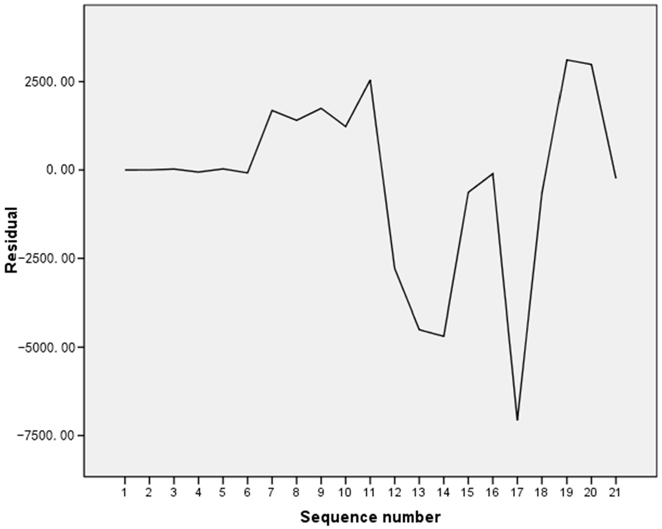
The residual sequence could be obtained by comparing the predicted results with the actual results presented in the second chapter, and the residual sequence diagrams could be drawn using SPSS software as shown in Figure 6.
3.3.2. Stationary Test of the Residual Sequence
The premise for establishing the ARIMA model for residual data is that the residual sequence needs to be stationary; therefore, it is necessary to test for the stability of the residual sequence. If the model is stationary, the model can be directly built. If it is not smooth, several orders of difference need to be made to stabilize it. The number of differences is indicated by the parameter d in the ARIMA model. Using SPSS software, the results of unit root tests for residual sequences are shown in Table 9.
Thus, the differential first-order sequence is stationary, and d = 1.
3.3.3. Autocorrelation Coefficients and Partial Autocorrelation Coefficients
After the parameter d was determined, it became necessary to determine the parameters p and q. The method for judging p and q has been introduced before, and the partial autocorrelation coefficient map was drawn via SPSS software, which is determined by the graph as follows.
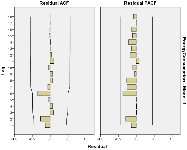
The diagrams as shown in Figure 7 and Figure 8 show that the autocorrelation coefficients and the partial autocorrelation coefficients of the residuals were all trailing; therefore, ARIMA (p, 1, q) models are chosen. The sequence was fitted via SPSS software, and the values of p and q were repeatedly determined. The confidence levels of the fitted sequences were compared between different p and q values, and following that, the final model type was determined as ARIMA (2,1,2). The parameters of the fitting result are shown in Table 10.
Therefore, the original residual sequence model is established as:
3.4. Test of the Built Model
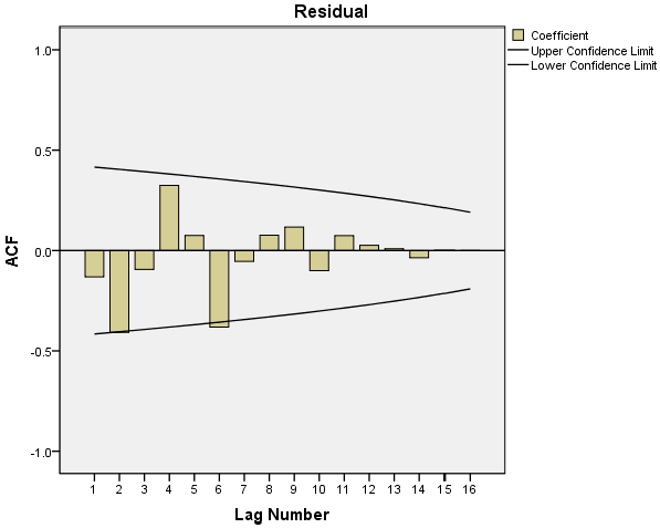
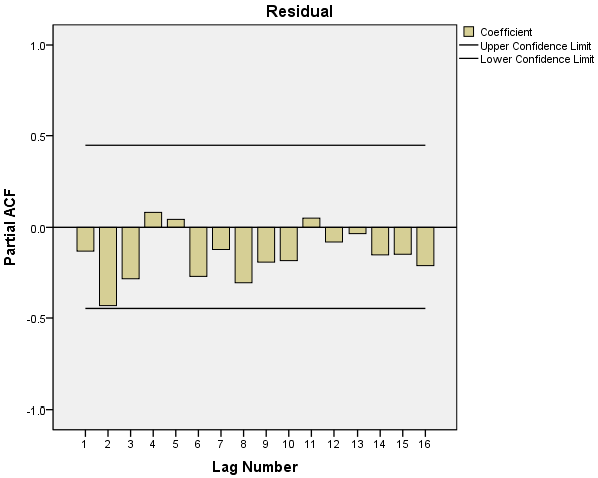
After the residuals have been fitted with the ARIMA (2,1,2) model, the residual sequence of residuals was obtained. The autocorrelation coefficients and the partial autocorrelation coefficients are shown as follows.
As shown in Figure 9, the fitted sequence is a white noise sequence; therefore, it could be used for prediction.
3.5. Prediction Results and Errors
The predicted results were combined with the residual corrected prediction, and finally the real prediction results were obtained. These were then compared to the true value, and the average relative error was calculated. After comparing the average relative error of the single prediction model as calculated in the second chapter, the advantages of this combination model over the single model prediction accuracy could be measured.
First, the metabolic GM (1,1) model was used to predict the error correction. Then, the ARIMA (2,1,2) model was used for the error correction. The predicted results are shown in Table 11.
Table 11 shows that the ARIMA model is capable of residual correction. The average relative error was 5.11%; therefore, the error was smaller and the prediction result was better. In combination with the above three methods, each accuracy could be calculated as shown in Table 12.
The results show that the average relative error of the GM-ARIMA composite model constructed in this paper was smaller than the resulting errors for each single model. Thus, we can conclude that the GM-ARIMA model has higher accuracy.
This analysis showed that the GM-ARIMA model can be used to forecast the energy demand of Shandong Province for the years of 2016–2020 and accurate forecast data can be obtained. The results are shown in Table 13.
4. Conclusions and Future Work
The GM-ARIMA model is very effective for systems with large sample size that follow trends, and it can be appropriately applied for the future energy prediction of Shandong province. This combination model was derived from the GM model and the ARIMA model. Through the improvement of the calculation process, we used the metabolic GM (1,1) model to predict the data. Then, the ARIMA model was used to obtain the results for residual correction. Finally, the residual correction process enabled further improvement in the accuracy of the predicted results on the original prediction. This was the major innovation of this study. Due to the complex data sequence of the energy demand, once the model was set up, we could use the currently available data to forecast the future data.
By analyzing and comparing the average relative error of different models, we found that the accuracies of GM (1,1), ARIMA (1,2,0), metabolic GM (1,1), and GM-ARIMA model were 44.38%, 6.309%, 6.57%, and 5.11%, respectively. It became obvious that the combination GM-ARIMA model has higher precision than each of the single models. The GM-ARIMA model combined advantages of both models, while avoiding their limitations. The advantage of the combination GM-ARIMA model is that it not only overcomes the shortcomings of the grey GM (1,1) model with less sample capacity, but also that it uses the ARIMA model to correct the prediction results and to improve accuracy. During the prediction process, the differential equation was used to determine the parameters, which provides a certain degree of accuracy and is more practical for non-stationary sequences. In summary, the results of energy consumption were reasonable.
The predicted results show that the energy consumption in Shandong province will still follow a slow upward trend in the future. A situation where the supply is not adequate to meet the demand may appear. To adapt to the increased energy demand, the government should take rational policy measures, increase investment in new energy technologies, promote energy structure adjustments, while at the same time, taking the development of green economic development into account.
The composite GM-ARIMA model provides a way to predict future energy consumption. This provides a reference value for future energy development planning, policy formulation, and technical direction. In the future, GM-ARIMA model predictions will be widely used in many areas: carbon emissions from fossil fuel combustion, energy shortages, economic development indicators, and a number of green energies. These forecasts are aimed at laying a solid foundation for the adjustment of energy structure and for the rational adjustment of the levels of both energy supply and demand. Through these efforts, we expect that the future energy development of Shandong will be more diversified, balanced, and orderly.
Acknowledgments
The current work is supported by “the Fundamental Research Funds for the Central Universities” (27R1706019B) and the Recruitment Talent Fund of China University of Petroleum (Huadong) (05Y16060020). We have received the grants in support of our research work. The funds we have received for covering the costs to publish in open access.
Author Contributions
Shuyu Li conceived and designed the experiments and wrote the paper and selected the data; Rongrong Li performed the experiments, analyzed the data and contributed reagents/materials/analysis tools. All authors read and approved the final manuscript.
Conflicts of Interest
The authors declare no conflicts of interest.
References
- Shandong Provincial Bureau of Statistics. Statistical Yearbook of Shangdong; China Statistics Press: Beijing, China, 2016. [Google Scholar]
- Shandong Provincial Bureau of Statistics. Statistical Yearbook of Shangdong; China Statistics Press: Beijing, China, 2010. [Google Scholar]
- Shandong Provincial Bureau of Statistics. Statistical Yearbook of Shangdong; China Statistics Press: Beijing, China, 2000. [Google Scholar]
- Zilberfarb, B.-Z.; Adams, F.G. The energy-gdp relationship in developing countries: Empirical evidence and stability tests. Energy Econ. 1981, 3, 244–248. [Google Scholar] [CrossRef]
- Wang, Q.; Li, R. Impact of cheaper oil on economic system and climate change: A SWOT analysis. Renew. Sustain. Energy Rev. 2016, 54, 925–931. [Google Scholar] [CrossRef]
- Wang, Q.; Li, R. Drivers for energy consumption: A comparative analysis of China and India. Renew. Sustain. Energy Rev. 2016, 62, 954–962. [Google Scholar] [CrossRef]
- Song, M.; Wang, S.; Yu, H.; Yang, L.; Wu, J. To reduce energy consumption and to maintain rapid economic growth: Analysis of the condition in China based on expended IPAT model. Renew. Sustain. Energy Rev. 2011, 15, 5129–5134. [Google Scholar] [CrossRef]
- Kraft, J.; Kraft, A. On the relationship between energy and GNP. J. Energy Dev. 1978, 3, 401–403. [Google Scholar]
- Akarca, A.T.; Long, T.V. On the relationship between energy and GNP: A reexamination. J. Energy Dev. 1980, 5, 326–331. [Google Scholar]
- Wolde-Rufael, Y. Energy consumption and economic growth: The experience of African countries revisited. Energy Econ. 2009, 31, 217–224. [Google Scholar] [CrossRef]
- Apergis, N.; Payne, J.E. Energy consumption and economic growth in Central America: Evidence from a panel cointegration and error correction model. Energy Econ. 2009, 31, 211–216. [Google Scholar] [CrossRef]
- Wang, Q.; Chen, X. Energy policies for managing China’s carbon emission. Renew. Sustain. Energy Rev. 2015, 50, 470–479. [Google Scholar] [CrossRef]
- Morris, S.; Goldstein, G.; Fthenakis, V. NEMS and MARKAL-MACRO models for energy-environmental-economic analysis: A comparison of the electricity and carbon reduction projections. Environ. Model. Assess. 2002, 7, 207–216. [Google Scholar] [CrossRef]
- Ireton-Jones, C.; Cnsd, F. Estimating energy requirements. In Nutritional Considerations in the Intensive Care Unit; Kendall/Hunt Publishing Co.: Dubuque, IA, USA, 2002; pp. 31–38. [Google Scholar]
- Srinivasan, D. Energy demand prediction using GMDH networks. Neurocomputing 2008, 72, 625–629. [Google Scholar] [CrossRef]
- Catalina, T.; Iordache, V.; Caracaleanu, B. Multiple regression model for fast prediction of the heating energy demand. Energy Build. 2013, 57, 302–312. [Google Scholar] [CrossRef]
- Box, G.E.; Jenkins, G.M.; Reinsel, G.C.; Ljung, G.M. Time Series Analysis: Forecasting and Control; John Wiley & Sons: Hoboken, NJ, USA, 2015. [Google Scholar]
- Deng, J.L. Grey System Fundamental Method; Huazhong University of Science and Technology: Wuhan, China, 1982. [Google Scholar]
- Wang, Q.; Li, R. Research status of shale gas: A review. Renew. Sustain. Energy Rev. 2017, 74, 715–720. [Google Scholar] [CrossRef]
- Wang, Q.; Li, R. Natural gas from shale formation: A research profile. Renew. Sustain. Energy Rev. 2016, 57, 1–6. [Google Scholar] [CrossRef]
- Wang, Q.; Chen, X.; Jha, A.N.; Rogers, H. Natural gas from shale formation—The evolution, evidences and challenges of shale gas revolution in United States. Renew. Sustain. Energy Rev. 2014, 30, 1–28. [Google Scholar] [CrossRef]
- Wang, Q. Effective policies for renewable energy—The example of China’s wind power—Lessons for China’s photovoltaic power. Renew. Sustain. Energy Rev. 2010, 14, 702–712. [Google Scholar] [CrossRef]
- Wang, Q. Nuclear safety lies in greater transparency. Nature 2013, 494, 403. [Google Scholar] [CrossRef] [PubMed]
- Morita, H.; Kase, T.; Tamura, Y.; Iwamoto, S. Interval prediction of annual maximum demand using grey dynamic model. Int. J. Electr. Power Energy Syst. 1996, 18, 409–413. [Google Scholar] [CrossRef]
- Rahimnia, F.; Moghadasian, M.; Mashreghi, E. Application of grey theory approach to evaluation of organizational vision. Grey Syst. Theory Appl. 2011, 1, 33–46. [Google Scholar] [CrossRef]
- Kayacan, E.; Ulutas, B.; Kaynak, O. Grey system theory-based models in time series prediction. Expert Syst. Appl. 2010, 37, 1784–1789. [Google Scholar] [CrossRef]
- Redclift, M. Sustainable Development: Exploring the Contradictions; Routledge: Abingdon, UK, 2002. [Google Scholar]
- Goosen, M.F.; Mahmoudi, H.; Ghaffour, N. Today’s and future challenges in applications of renewable energy technologies for desalination. Crit. Rev. Environ Sci. Technol. 2014, 44, 929–999. [Google Scholar] [CrossRef]
- Crabtree, G.; Kocs, E.; Aláan, T. Energy, society and science: The fifty-year scenario. Futures 2014, 58, 53–65. [Google Scholar] [CrossRef]
- Pai, P.-F.; Lin, C.-S. A hybrid ARIMA and support vector machines model in stock price forecasting. Omega 2005, 33, 497–505. [Google Scholar] [CrossRef]
- Sowell, F. Modeling long-run behavior with the fractional ARIMA model. J. Monet. Econ. 1992, 29, 277–302. [Google Scholar] [CrossRef]
- Tseng, F.-M.; Tzeng, G.-H.; Yu, H.-C.; Yuan, B.J. Fuzzy ARIMA model for forecasting the foreign exchange market. Fuzzy Sets Syst. 2001, 118, 9–19. [Google Scholar] [CrossRef]
- Bowden, N.; Payne, J.E. Short term forecasting of electricity prices for MISO hubs: Evidence from ARIMA-EGARCH models. Energy Econ. 2008, 30, 3186–3197. [Google Scholar] [CrossRef]
- Ediger, V.Ş.; Akar, S. ARIMA forecasting of primary energy demand by fuel in Turkey. Energy Policy 2007, 35, 1701–1708. [Google Scholar] [CrossRef]
- Pappas, S.S.; Ekonomou, L.; Karamousantas, D.C.; Chatzarakis, G.; Katsikas, S.; Liatsis, P. Electricity demand loads modeling using AutoRegressive Moving Average (ARMA) models. Energy 2008, 33, 1353–1360. [Google Scholar] [CrossRef]
- Saab, S.; Badr, E.; Nasr, G. Univariate modeling and forecasting of energy consumption: The case of electricity in Lebanon. Energy 2001, 26, 1–14. [Google Scholar] [CrossRef]
- Sen, P.; Roy, M.; Pal, P. Application of ARIMA for forecasting energy consumption and GHG emission: A case study of an Indian pig iron manufacturing organization. Energy 2016, 116, 1031–1038. [Google Scholar] [CrossRef]
- Hidalgo, L.M.R.; Peralta-Suárez, L.M.; Busto Yera, Y. Development of a technology for treating wastewater contaminated with nitric acid. J. Waste Manag. 2013, 2013, 1–7. [Google Scholar] [CrossRef]
- Australian Capital Territory. W.T.C.T.A.C.C.S. 2007. Available online: http://www.tams.act.gov.au/__data/assets/pdf_file/0003/63624/Climate_Change_Strategy.pdf (accessed on 30 June 2017).
- Bangkok Metropolitan Administration. Action Plan on Global Warming Mitigation 2007–2012. Available online: http://baq2008.org/system/files/BMA+Plan.pdf (accessed on 30 June 2017).
- Allwood, J.M.; Cullen, J.M.; Milford, R.L. Options for achieving a 50% cut in industrial carbon emissions by 2050. Environ. Sci. Technol. 2010. [Google Scholar] [CrossRef] [PubMed]
- Wang, Q. Cheaper Oil—Challenge and Opportunity for Climate Change. Environ. Sci. Technol. 2015, 49, 1997–1998. [Google Scholar] [CrossRef] [PubMed]
- Wang, Q. China’s citizens must act to save their environment. Nature 2013, 497, 159. [Google Scholar] [CrossRef] [PubMed]
- Wang, Q. China has the capacity to lead in carbon trading. Nature 2013, 493, 273. [Google Scholar] [CrossRef] [PubMed]
- Faruk, D.Ö. A hybrid neural network and ARIMA model for water quality time series prediction. Eng. Appl. Artif. Intell. 2010, 23, 586–594. [Google Scholar] [CrossRef]
- Conejo, A.J.; Plazas, M.A.; Espinola, R.; Molina, A.B. Day-ahead electricity price forecasting using the wavelet transform and ARIMA models. IEEE Trans. Power Syst. 2005, 20, 1035–1042. [Google Scholar] [CrossRef]
- Gregory, A.W.; Hansen, B.E. Residual-based tests for cointegration in models with regime shifts. J. Econ. 1996, 70, 99–126. [Google Scholar] [CrossRef]
- Gerolimetto, M.; Magrini, S. On the power of the simulation-based ADF test in bounded time series. Econ. Bull. 2017, 37, 539–552. [Google Scholar]
- Wang, Q.; Li, R.; Jiang, R. Decoupling and Decomposition Analysis of Carbon Emissions from Industry: A Case Study from China. Sustainability 2016, 8, 1059. [Google Scholar] [CrossRef]
- Lehtikangas, O.; Vauhkonen, M. Correlated noise and prior models in electromagnetic flow tomography. Meas. Sci. Technol. 2017, 28, 054007. [Google Scholar] [CrossRef]
- De la Torre, S.; Conejo, A.; Contreras, J. Simulating oligopolistic pool-based electricity markets: A multiperiod approach. IEEE Trans. Power Syst. 2003, 18, 1547–1555. [Google Scholar] [CrossRef]
- Lee, Y.-S.; Tong, L.-I. Forecasting energy consumption using a grey model improved by incorporating genetic programming. Energy Convers. Manag. 2011, 52, 147–152. [Google Scholar] [CrossRef]
- Kumar, U.; Jain, V. Time series models (Grey-Markov, Grey Model with rolling mechanism and singular spectrum analysis) to forecast energy consumption in India. Energy 2010, 35, 1709–1716. [Google Scholar] [CrossRef]
- Wang, Q.; Li, R.; Liao, H. Toward Decoupling: Growing GDP without Growing Carbon Emissions. Environ. Sci. Technol. 2016, 50, 11435–11436. [Google Scholar] [CrossRef] [PubMed]
- Wang, Q.; Jiang, X.-T.; Li, R. Comparative decoupling analysis of energy-related carbon emission from electric output of electricity sector in Shandong Province, China. Energy 2017, 127, 78–88. [Google Scholar] [CrossRef]
- Wang, Q.; Li, R. Sino-Venezuelan oil-for-loan deal—The Chinese strategic gamble? Renew. Sustain. Energy Rev. 2016, 64, 817–822. [Google Scholar] [CrossRef]
- Wang, Q.; Li, R. Journey to burning half of global coal: Trajectory and drivers of China’s coal use. Renew. Sustain. Energy Rev. 2016, 58, 341–346. [Google Scholar] [CrossRef]
- Wang, Q.; Li, R. Decline in China’s coal consumption: An evidence of peak coal or a temporary blip? Energy Policy 2017, 108, 696–701. [Google Scholar] [CrossRef]
- Akay, D.; Atak, M. Grey prediction with rolling mechanism for electricity demand forecasting of Turkey. Energy 2007, 32, 1670–1675. [Google Scholar] [CrossRef]
- Dounis, A.; Tiropanis, P.; Tseles, D.; Nikolaou, G.; Syrcos, G. A comparison of grey model and fuzzy predictive model for time series. Environ. Sci. 2006, 6, 8–15. [Google Scholar]
- Hsu, C.-C.; Chen, C.-Y. Applications of improved grey prediction model for power demand forecasting. Energy Convers. Manag. 2003, 44, 2241–2249. [Google Scholar] [CrossRef]
- Zhu-xin, Y. A GM (1,1) the Model for the Income Adisparity Forecast in China. Math. Pract. Theory 2007, 10, 006. [Google Scholar]
- Kearney, M.R.; Wintle, B.A.; Porter, W.P. Correlative and mechanistic models of species distribution provide congruent forecasts under climate change. Conserv. Lett. 2010, 3, 203–213. [Google Scholar] [CrossRef]
- Jaeger, H.; Haas, H. Harnessing nonlinearity: Predicting chaotic systems and saving energy in wireless communication. Science 2004, 304, 78–80. [Google Scholar] [CrossRef] [PubMed]
- Tsonis, A.; Elsner, J. Nonlinear prediction as a way of distinguishing chaos from random fractal sequences. Nature 1992, 358, 217–220. [Google Scholar] [CrossRef]
- Onuchic, J.N.; Wolynes, P.G. Theory of protein folding. Curr. Opin. Struct. Biol. 2004, 14, 70–75. [Google Scholar] [CrossRef] [PubMed]
- Peirong, J.; Xiangyong, H.; Dongqing, X. Analysis and Evaluation to grey forecasting model. Hydroelectr. Energy 1999, 17, 42–44. [Google Scholar]
Figure 1.
Autocorrelation and partial autocorrelation function diagram of energy demand in Shandong Province. (a) indicated that the autocorrelation function is tailed; (b) indicated that the partial autocorrelation function is truncated.
Figure 1.
Autocorrelation and partial autocorrelation function diagram of energy demand in Shandong Province. (a) indicated that the autocorrelation function is tailed; (b) indicated that the partial autocorrelation function is truncated.
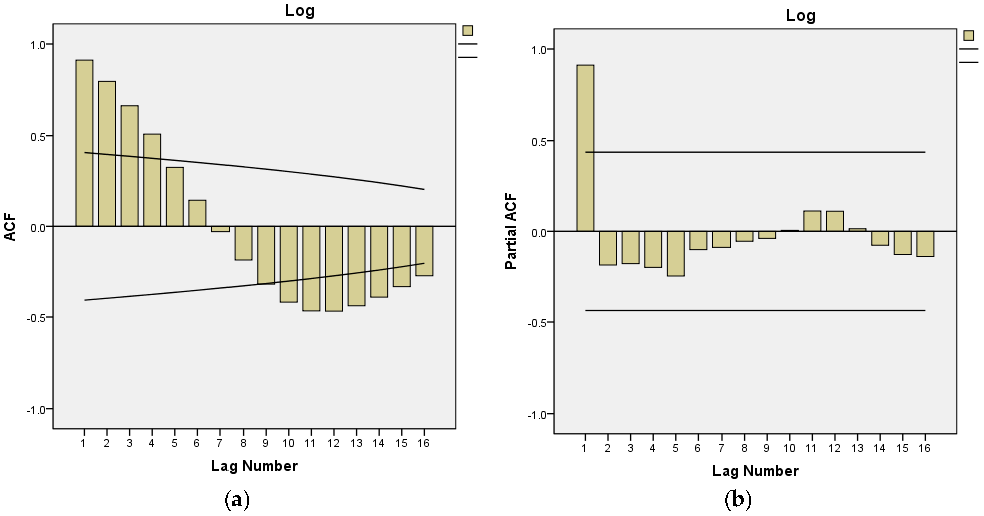
Figure 2.
The autocorrelation and partial autocorrelation maps of the residuals.

Figure 3.
The fitting prediction based on ARIMA model. Note: “UCL” means upper control line; “LCL” means lower control line.
Figure 3.
The fitting prediction based on ARIMA model. Note: “UCL” means upper control line; “LCL” means lower control line.

Figure 4.
Raw data sequence diagram.
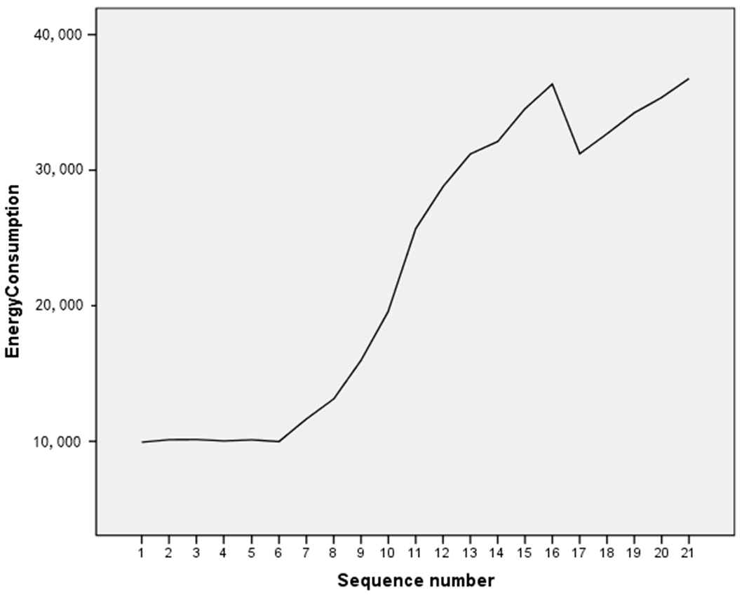
Figure 5.
Raw data histogram.

Figure 6.
The residual sequence.

Figure 7.
Autocorrelation function of residual sequence.

Figure 8.
Partial autocorrelation function of residual sequence.

Figure 9.
Autocorrelation coefficients and partial autocorrelation coefficients of residual residuals.
Figure 9.
Autocorrelation coefficients and partial autocorrelation coefficients of residual residuals.


Table 1.
The energy consumption of Shandong province from 1995 to 2015.
| Year | Energy Consumption/Tons of Standard Coal |
|---|---|
| 1995 | 9938.71 |
| 1996 | 10,117.67 |
| 1997 | 10,128.81 |
| 1998 | 10,028.80 |
| 1999 | 10,104.56 |
| 2000 | 9977.11 |
| 2001 | 11,649.88 |
| 2002 | 13,121.91 |
| 2003 | 15,974.50 |
| 2004 | 19,606.14 |
| 2005 | 25,687.50 |
| 2006 | 28,786.10 |
| 2007 | 31,194.99 |
| 2008 | 32,116.22 |
| 2009 | 34,535.66 |
| 2010 | 36,357.25 |
| 2011 | 31,211.80 |
| 2012 | 32,686.70 |
| 2013 | 34,234.90 |
| 2014 | 35,362.60 |
| 2015 | 36,759.20 |
Table 2.
The stationarity test of energy demand time series in Shandong Province.
| Sequence | ADF Statistic | Critical Value | Value of p | ||
|---|---|---|---|---|---|
| 1% | 5% | 10% | |||
| Q | −3.648121 | −4.667883 | −3.733200 | −3.310349 | 0.0577 |
| Q* | −2.280862 | −4.532598 | −3.673616 | −3.277364 | 0.4233 |
| Q** | −5.709960 | −4.571559 | −3.690814 | −3.286909 | 0.0012 |
Note: Augmented Dickey Fuller (ADF). Q* is the first order difference of Q. Q** is the two-order difference of Q.
Table 3.
The basic principles of model recognition.
| Autocorrelation Function | Partial Autocorrelation Function | Type of Model |
|---|---|---|
| Trailing | P order truncation | AR (p) |
| Q order truncation | Trailing | MA (q) |
| Trailing | Trailing | ARMA (p, q) |
Table 4.
Model Statistics.
| Model | Stationary R Squared | Sig. | Number of Outliers |
|---|---|---|---|
| Energy Consumption | 0.162 | 0.976 | 0 |
Table 5.
ARIMA Model Parameters.
| Model | Constant | AR(Lag1) | Difference | Numerator |
|---|---|---|---|---|
| Energy Consumption | 47,096.394 | −0.382 | 2 | −23.446 |
Table 6.
The prediction results and residual values of GM (1,1) model.
| Year | Actual Value/Tons of Standard Coal | Predicted Value/Tons of Standard Coal | Residual/Tons of Standard Coal | Relative Error |
|---|---|---|---|---|
| 1995 | 9938.71 | 9938.71 | 0 | 0% |
| 1996 | 10,117.67 | 10,115.627 | −2.0432 | 0.02% |
| 1997 | 10,128.81 | 10,101.475 | −27.3351 | 0.27% |
| 1998 | 10,028.80 | 10,087.343 | 58.5426 | 0.58% |
| 1999 | 10,104.56 | 10,073.23 | −31.3297 | 0.31% |
| 2000 | 9977.11 | 10,059.138 | 82.0276 | 0.82% |
| 2001 | 11,649.88 | 10,045.065 | −1604.82 | 13.78% |
| 2002 | 13,121.91 | 10,031.012 | −3090.9 | 23.56% |
| 2003 | 15,974.50 | 10,016.978 | −5957.52 | 37.29% |
| 2004 | 19,606.14 | 10,002.964 | −9603.18 | 48.98% |
| 2005 | 25,687.50 | 9988.9695 | −15,698.5 | 61.11% |
| 2006 | 28,786.10 | 9974.9948 | −18,811.1 | 65.35% |
| 2007 | 31,194.99 | 9961.0395 | −21,234 | 68.07% |
| 2008 | 32,116.22 | 9947.1039 | −22,169.1 | 69.03% |
| 2009 | 34,535.66 | 9933.1876 | −24,602.5 | 71.24% |
| 2010 | 36,357.25 | 9919.2909 | −26,438 | 72.72% |
| 2011 | 31,211.80 | 9905.4136 | −21,306.4 | 68.26% |
| 2012 | 32,686.70 | 9891.5558 | −22,795.1 | 69.74% |
| 2013 | 34,234.90 | 9877.7172 | −24,357.2 | 71.15% |
| 2014 | 35,362.60 | 9863.8981 | −25,498.7 | 72.11% |
| 2015 | 36,759.20 | 9850.0984 | −26,909.1 | 73.20% |
Table 7.
The sum of squares of residuals of each dimension.
| Dimension | ||||||
|---|---|---|---|---|---|---|
| Sum of Squares of Residuals | 5 | 6 | 7 | 8 | 9 | 10 |
| 135,452,583 | 166,026,131 | 209,743,846 | 274,770,956 | 345,088,570 | 409,611,901 | |
Table 8.
Trend item fitting results.
| Year | Predicted Value/Tons of Standard Coal | True Value/Tons of Standard Coal | Absolute Error/Tons of Standard Coal | Relative Error |
|---|---|---|---|---|
| 1995 | 9938.71 | 9938.71 | 0 | 0.00% |
| 1996 | 10,115.63 | 10,117.67 | 2.04 | 0.02% |
| 1997 | 10,101.47 | 10,128.81 | 27.34 | 0.27% |
| 1998 | 10,087.34 | 10,028.8 | 58.54 | 0.58% |
| 1999 | 10,073.23 | 10,104.56 | 31.33 | 0.31% |
| 2000 | 10,059.14 | 9977.11 | 82.028 | 0.82% |
| 2001 | 9963.672 | 11,649.88 | 1686.208 | 14.47% |
| 2002 | 11,717.69 | 13,121.91 | 1404.219 | 10.70% |
| 2003 | 14,228.42 | 15,974.5 | 1746.084 | 10.93% |
| 2004 | 18,377.62 | 19,606.14 | 1228.516 | 6.27% |
| 2005 | 23,139.35 | 25,687.5 | 2548.148 | 9.92% |
| 2006 | 31,575.46 | 28,786.1 | 2789.358 | 9.69% |
| 2007 | 35,700.99 | 31,194.99 | 4506 | 14.44% |
| 2008 | 36,807.63 | 32,116.22 | 4691.409 | 14.61% |
| 2009 | 35,166.92 | 34,535.66 | 631.259 | 1.83% |
| 2010 | 36,460.9 | 36,357.25 | 103.649 | 0.29% |
| 2011 | 38,279.69 | 31,211.8 | 7067.891 | 22.64% |
| 2012 | 33,350.04 | 32,686.7 | 663.335 | 2.03% |
| 2013 | 31,120.65 | 34,234.9 | 3114.254 | 9.10% |
| 2014 | 32,375.9 | 35,362.6 | 2986.705 | 8.45% |
| 2015 | 36,998.49 | 36,759.2 | 239.292 | 0.65% |
Table 9.
Unit root tests for residual sequences.
| Sequences | ADF Statistic | Critical Value | Value of p | ||
|---|---|---|---|---|---|
| 1% | 5% | 10% | |||
| Q | −2.821063 | −4.498307 | −3.658446 | −3.268973 | 0.2064 |
| Q* | −4.500677 | −4.571559 | −3.690814 | −3.286909 | 0.0114 |
Note: Q* is the first order difference of Q.
Table 10.
ARIMA Model Parameters.
| Model | Constant | AR (Lag2) | MA (Lag2) | Difference | Numerator |
|---|---|---|---|---|---|
| Energy Consumption | −12,695.083 | −0.841 | −0.653 | 1 | 6.381 |
Table 11.
Prediction results and errors.
| Year | Predicted Value/Tons of Standard Coal | Residual Prediction/Tons of Standard Coal | Final Predicted Value/Tons of Standard Coal | True Value/Tons of Standard Coal | Absolute Error/Tons of Standard Coal | Relative Error |
|---|---|---|---|---|---|---|
| 1995 | 9938.71 | 0 | 9938.71 | 9938.71 | 0 | 0.00% |
| 1996 | 10,115.63 | −39.98 | 10,075.65 | 10,117.67 | 42.02 | 0.42% |
| 1997 | 10,101.47 | −28.42 | 10,073.05 | 10,128.81 | 55.76 | 0.55% |
| 1998 | 10,087.34 | −164.08 | 9923.26 | 10,028.8 | 105.54 | 1.05% |
| 1999 | 10,073.23 | −33.04 | 10,040.19 | 10,104.56 | 64.37 | 0.64% |
| 2000 | 10,059.14 | −232.11 | 9827.028 | 9977.11 | 150.082 | 1.50% |
| 2001 | 9963.672 | 1655.47 | 11,619.142 | 11,649.88 | 30.7384 | 0.26% |
| 2002 | 11,717.69 | 113.77 | 11,831.461 | 13,121.91 | 1290.449 | 9.83% |
| 2003 | 14,228.42 | 795.83 | 15,024.246 | 15,974.5 | 950.254 | 5.95% |
| 2004 | 18,377.62 | −594.97 | 17,782.654 | 19,606.14 | 1823.486 | 9.30% |
| 2005 | 23,139.35 | 746.24 | 23,885.592 | 25,687.5 | 1801.908 | 7.01% |
| 2006 | 31,575.46 | −5471.41 | 26,104.048 | 28,786.1 | 2682.052 | 9.32% |
| 2007 | 35,700.99 | −2985.75 | 32715.24 | 31,194.99 | 1520.25 | 4.87% |
| 2008 | 36,807.63 | −2557.42 | 34,250.209 | 32,116.22 | 2133.99 | 6.64% |
| 2009 | 35,166.92 | 2935.6 | 38,102.519 | 34,535.66 | 3566.86 | 10.33% |
| 2010 | 36,460.9 | 2443.12 | 38,904.019 | 36,357.25 | 2546.77 | 7.00% |
| 2011 | 38,279.69 | −4395.04 | 33,884.651 | 31,211.8 | 2672.85 | 8.56% |
| 2012 | 33,350.04 | 4375.3 | 37,725.335 | 32,686.7 | 5038.64 | 15.41% |
| 2013 | 31,120.65 | 1366.99 | 32,487.636 | 34,234.9 | 1747.264 | 5.10% |
| 2014 | 32,375.9 | 1931.19 | 34,307.085 | 35,362.6 | 1055.515 | 2.98% |
| 2015 | 36,998.49 | −30.94 | 36,967.552 | 36,759.2 | 208.352 | 0.57% |
Table 12.
Comparison results of different methods.
| Method | Average Relative Error |
|---|---|
| GM (1,1) | 44.38% |
| ARIMA (1,2,0) | 6.309% |
| Metabolism GM (1,1) | 6.57% |
| GM-ARIMA | 5.11% |
Table 13.
Forecast data of energy demand in Shandong in 2016–2020.
| Year | Energy Demand in Shandong/Tons of Stadard Coal |
|---|---|
| 2016 | 38,208.307 |
| 2017 | 39,700.07 |
| 2018 | 41,250.076 |
| 2019 | 42,860.598 |
| 2020 | 44,534 |
© 2017 by the authors. Licensee MDPI, Basel, Switzerland. This article is an open access article distributed under the terms and conditions of the Creative Commons Attribution (CC BY) license (http://creativecommons.org/licenses/by/4.0/).
Share and Cite
MDPI and ACS Style
Li, S.; Li, R. Comparison of Forecasting Energy Consumption in Shandong, China Using the ARIMA Model, GM Model, and ARIMA-GM Model. Sustainability 2017, 9, 1181. https://doi.org/10.3390/su9071181
AMA Style
Li S, Li R. Comparison of Forecasting Energy Consumption in Shandong, China Using the ARIMA Model, GM Model, and ARIMA-GM Model. Sustainability. 2017; 9(7):1181. https://doi.org/10.3390/su9071181
Chicago/Turabian StyleLi, Shuyu, and Rongrong Li. 2017. "Comparison of Forecasting Energy Consumption in Shandong, China Using the ARIMA Model, GM Model, and ARIMA-GM Model" Sustainability 9, no. 7: 1181. https://doi.org/10.3390/su9071181
Note that from the first issue of 2016, this journal uses article numbers instead of page numbers. See further details here.