Multi-Objective Spatial Optimization: Sustainable Land Use Allocation at Sub-Regional Scale
by
Guadalupe Azuara García
1,*, 
Efrén Palacios Rosas
2,
Alfonso García-Ferrer
3 and
Pilar Montesinos Barrios
1 1
Department of Agronomy, University of Cordoba, Rabanales Campus. Ed. 14071 Córdoba, Spain
2
Freelance consultant in computing languages, Cordillera Central 2428, Fraccionamiento Maravillas Puebla Pue Z.C. 72220, Mexico
3
Gregor Mendel, Z.C. 14071 Córdoba, Spain
*
Author to whom correspondence should be addressed.
Sustainability 2017, 9(6), 927; https://doi.org/10.3390/su9060927
Submission received: 16 February 2017
/
Revised: 24 May 2017
/
Accepted: 25 May 2017
/
Published: 1 June 2017
(This article belongs to the Section Environmental Sustainability and Applications)
Abstract
:The rational use of territorial resources is a key factor in achieving sustainability. Spatial planning is an important tool that helps decision makers to achieve sustainability in the long term. This work proposes a multi-objective model for sustainable land use allocation known as MAUSS (Spanish acronym for “Modelo de Asignación de Uso Sostenible de Suelo”) The model was applied to the Plains of San Juan, Puebla, Mexico, which is currently undergoing a rapid industrialization process. The main objective of the model is to generate land use allocations that lead to a territorial balance within regions in three main ways by maximizing income, minimizing negative environmental pressure on water and air through specific evaluations of water use and CO2 emissions, and minimizing food deficit. The non-sorting genetic algorithm II (NSGA-II) is the evolutionary optimization algorithm of MAUSS. NSGA-II has been widely modified through a novel and efficient random initializing operator that enables spatial rationale from the initial solutions, a crossover operator designed to streamline the best genetic information transmission as well as diversity, and two geometric operators, geographic dispersion (GDO) and the proportion (PO), which strengthen spatial rationality. MAUSS provided a more sustainable land use allocation compared to the current land use distribution in terms of higher income, 9% lower global negative pressure on the environment and 5.2% lower food deficit simultaneously.
1. Introduction
Land use allocation has been an inherent practice for developing human productive activities throughout the world. However, the main issue currently faced by spatial planners and society as a whole is that such allocations must be profitable, but preserve life on earth, that is, promote an environmental, social and economic equilibrium. Land use assignments must be sustainable. Thus far, few works have included sustainability criteria and they are practically non-existent in poor and developing countries. Nevertheless, sustainable land use allocations are critical for averting irreversible environmental disasters related to the use and exploitation of territories, as has already occurred in Amazon forest devastation [1] or the disappearance of the Aral Sea [2], and may happen in territories with a strong potential for land use change.
Although the concept of sustainability can be addressed in different manners depending on specific territorial problems, spatial planners are increasingly concerned about yielding a territorial balance capable of improving the current land occupation depending on the geographical extent and the stakeholders’ goals from an all-encompassing approach. In this respect, issues such as CO2 emissions, soil erosion, the nature value of the area, land use change expenses, and land use suitability, among others, have been included as the environmental component of spatial planning models [3,4,5,6,7]. However, these models have not considered water resources evaluation, which is indispensable for comprehensive planning [8]. It is undeniable that social benefits may result from achieving environmental and economic targets; nonetheless, social objectives have been lacking in spatial planning until now. In this sense, the present research includes food security (according to the FAO definition [9]) as an important social component for achieving land use sustainability. This social goal is considered an objective function in terms of minimizing food deficit rather than an area constraint [10,11].
The work of planners has been greatly aided by the development of computer applications to facilitate the processing of large amounts of spatial and non-spatial data, as well as the introduction of methods and techniques to improve the optimization process of land use allocation. In this regard, a vast range of broadly documented computational methods and tools has been developed, from linear programming (LP) for one or several objectives [12,13,14,15] to heuristic multiple-objective models, among them evolutionary algorithms (MOEAs) [3,16]. MOEAs do not search for a single solution but rather a set of feasible solutions (the Pareto front) that compensate several frequently opposing objectives, such as competing land uses. Moreover, due to their enhanced and less restricted performance in comparison to LPs, MOEAs are a helpful tool for decision makers.
Evolutionary algorithms have become a wide spread and developed tool due to their high adaptive capacity to solve many different types of problems, such as hydraulic engineering applications [17,18], hospital management optimization [19] or spatial planning [5]. Most of them are bioinspired or nature-based, such as the genetic, immunological, swarm and ant colony algorithms [20,21,22,23,24]. When combining these algorithms with other computer, geographical, statistical and mathematical tools, they gain effectiveness and become powerful search engines for optimal solutions.
Genetic algorithms (GA) have been used in spatial planning since the 1990s to evaluate territorial information through vector-based [25] or grid-based representations [4], generally assisted by geographical information systems (GIS). Since they were first developed, the resolution of both representations has improved, although GIS has undergone more significant improvements from schematic representations of huge cell size [26] to the current accurate representations with very small cell size grid of the accessible cartographic sources [11], thus permitting better assessment and land use allocation. Nonetheless, resolution continues to depend on the geographical extent.
In contrast to other non-spatial applications, the main challenge to GAs in land use allocation is not only to obtain an optimum solution set according to the model objective functions, but also to obtain a spatially coherent set from a strong randomization procedure with random decision variables, which is needed for simulating evolutionary processes of living beings. To overcome this problem, researchers have opted in practice for one of two options: (1) to include, from the spatial geometry perspective [27], the geometric objectives as objective functions in order to optimize land use size and compactness; and (2) to use, adjust and even create new genetic operators to achieve geometric objectives, and save objective functions as final targets in the spatial planning process.
From the first perspective, which is more useful at the local scale, several works have been made [28,29] exhibiting good computing and spatial results, but also an enormous territorial assessment simplification, which has been restricted to a single suitability or fitness function. From the second approach, preferred in this research, where the allocation of a cell or polygon land use is dealt as a combinatory optimization problem or as an Integer Programming problem [5], there have been excellent quantitative and spatial distribution results [30] for diverse work scales (local and regional) and a more detailed territorial assessment through objective functions which lead to better land use allocations. Both GA approaches have incorporated additional procedures, such as game theory [11], parallel algorithms [29], goal programming or weighted sum method [4], thus becoming a fundamental component in spatial decision support systems.
As an improved multi-objective genetic algorithm, the non-sorting genetic algorithm II (NSGA-II) [31] has been used for spatial planning [3,5,6]. In this work, the NSGA-II has been applied as an optimization procedure due to its efficiency and effectiveness in selecting feasible and better solutions through generations, even though important modifications have been made. On the one hand, the modified NSGA-II includes an improved mechanism of population initialization that ensures compactness; on the other hand, new genetic operators responsible for land use contiguity and size through generations have been designed, in a way that facilitates land use allocation problem when incorporating planner guidelines.
As an integer programming problem approach with a work scale larger than local (sub-regional), this research is able to assess many spatial characteristics that cannot be constricted in just one function. Objective functions are therefore seen as a means to achieve global planners’ objectives, while genetic operators are seen as key factors for achieving diversity and geometric objectives simultaneously.
In this work, a multi-objective model for sustainable land use allocation is proposed. The main goal of the model is to generate land use allocations that lead to a territorial balance within a region considering three objectives: maximizing income, minimizing negative environmental pressure on water and air and minimizing food deficit. The search for optimal solutions is carried out using a modified version of the NSGA-II algorithm in which the generation process of initial solutions and the genetic operators have been changed. The algorithm also includes two geometric operators in order to strengthen spatial rationality. Finally, the model is applied to the Plains of San Juan (Puebla), in the heart of Mexico, to compare several sustainable solutions derived from the proposed model with the current land use allocation.
2. Materials and Methods
2.1. Problem Formulation
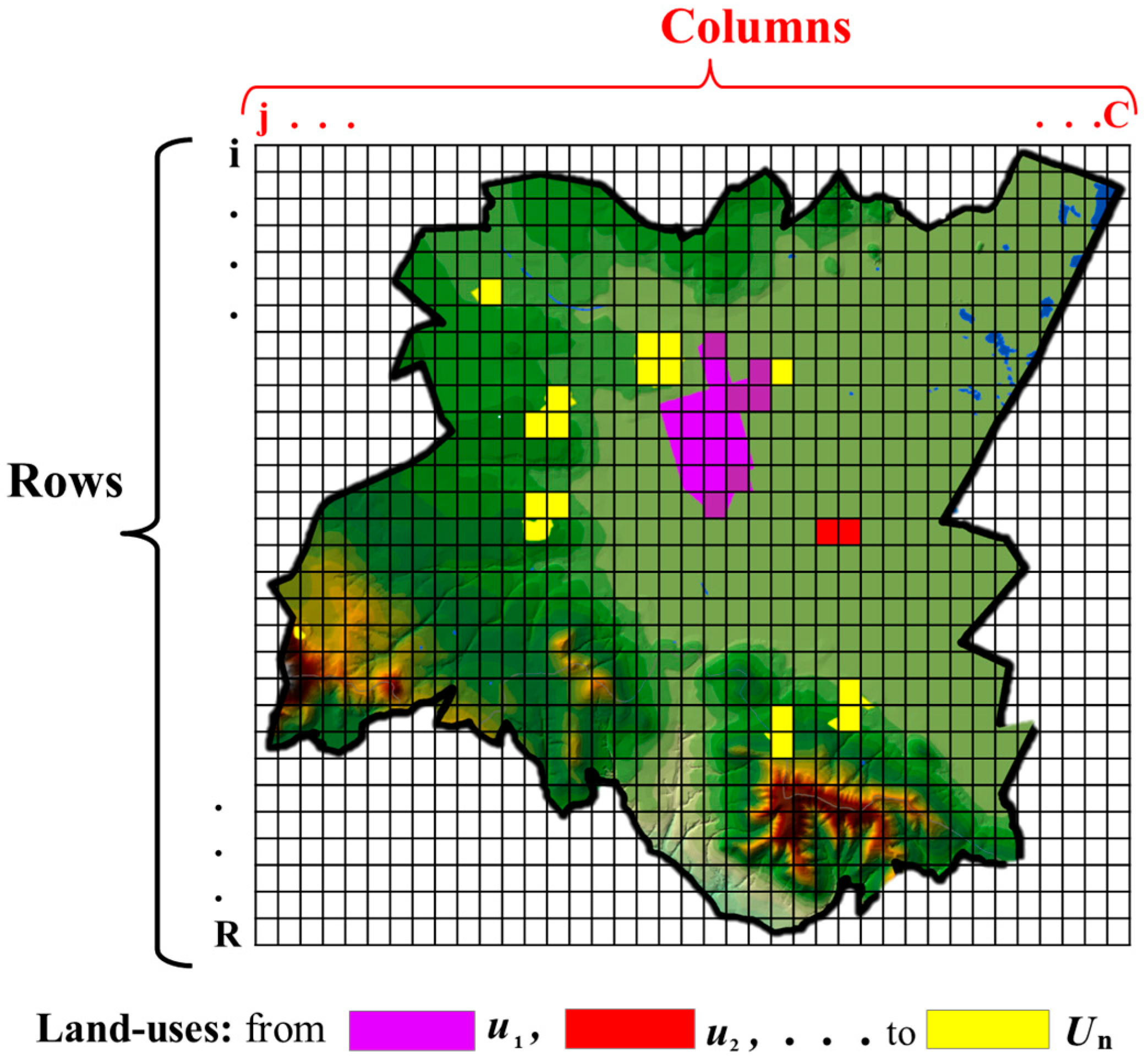
The following multi-objective optimization problem aims to provide a sustainable territorial exploitation at the sub-region scale considering economic, environmental and social aspects and an annual time scale. For land use allocation, the territorial discretization into homogeneous cells (Figure 1) according to the detail of available spatial data in raster format has been adopted. Each cell is a square portion of the territory with a single land use. Territory spatial features are analyzed in each grid cell.
2.1.1. Income Maximization
Despite the fact that it is not possible to generalize social well-being based solely on income, it is still a key indicator of the wealth generated by each land use. Hence it is important to include this indicator as a maximization objective, provided that it is limited by sustainability parameters to minimize man-made geographical unbalances’ on earth. Many spatial optimization works have included, in different manners, economic aspects as an objective function, which are conceived as the minimization of land use conversion costs [3,30] or the maximization of economic return [5]. In this particular case, we have defined the following equation to evaluate territorial income:
Minimize:
where is a binary decision variable that allocates only one land use type u to the cell located in row i, column j; is land use type from u to U; R denotes the rows of the grid from i to R; C is the columns of the grid from j to C; is the annual average income (millions of currency units) of cell ij with land use u; is the maximum income possible for cell ij; and is the territorial aptitude factor for land use u allocated in cell ij from 0.5 to 1. The latter is a parameter model utilized in the three objective functions and only affects land uses directly linked to food production; namely cropland (rain fed/irrigated) and grassland according to land aptitude and the historical yields recorded in the study area. For the remaining land uses, this factor is 1.
The average income per surface unit (cell) is obtained by dividing income per activity (land use) by its area. The result of this operation is given in currency units. Thus, in order to facilitate comparisons among the objective functions in the solution space, it is transformed into a ratio when divided by the summation of maximum possible income of all cells. The value of the O1 function, which is expressed in dimensionless units (DU), ranges from 0 to 4.
2.1.2. Minimizing Negative Pressures on the Environment
Sustainable land uses are required to preserve our environment. Thus, as a novel approach to achieve sustainability from a territorial planning perspective, an objective function targeted at minimizing the negative pressures of land uses on water and air is included. At the sub-regional level, the aim is to evaluate, in a simplified way, which land use allocations prove to be more environmentally friendly than others.
Each type of land use exerts pressure on water resources due to over exploitation and deterioration of water quality. The former can be analyzed using the water footprint (WF) concept [32]. This concept is defined as the total volume of freshwater required to obtain a product or carry out an activity, which is accounted for throughout the fully supply chain. WF is a comprehensive indicator of freshwater resource appropriation that varies geographically and temporally and is used to assess the polluting potential per land use.
The pressures on air exerted by different land uses are evaluated using the concept of carbon footprint that quantifies Green House Gases (GHG) in terms of CO2 equivalent, which constitutes the main cause of global warming, climate change and environmental imbalance (including biodiversity loss).
By including function O2, which summarizes negative pressures on the environment (water and air), it is possible to find territorial distributions of land uses that preserve water bodies (surface and ground waters) and produce less CO2 emissions by improving accessibility to certain land uses, promoting industrial and urban use compactness and reducing land use changes (e.g., from forestry to urban use). The objective function O2 is expressed as follows.
Minimize:
where PWuij is the dimensionless negative pressure on water and PAuij is the negative pressure on air. PWuij is calculated according to the following equation that combines pressures related to water demand and quality in the first and second summand, respectively:
where is the annual water availability (m3/cell·yr) in cell ij, is the water footprint (m3/cell·yr) for use u in cell ij; and is the previously defined territorial aptitude factor of cell ij for land use u which only affects cropland and grassland according to land aptitude. WFu was calculated from public data sets (global, national and local statistics, basin authorities’ data, corporation reports, etc.). It is the summation of green and blue water footprints according to the origin of the water (green water is the fraction of rainfall stored in soils and blue water represents the withdrawal from water bodies). Thereby, urban WF can be estimated from the population census and urban densities, while industrial WF varies according to the type of product, manufacturing process and production. In this work, only industrial WF in industries has been considered. For agricultural, grassland and forestry land uses their WF is the summation of blue and green WFs as they may be rain fed and/or irrigated land use types. Green WFs were calculated using the free software CROPWAT developed by FAO based on Allen et al. [33] due to its suitability for performing green WF calculations for products of plant origin [32,34,35]. Blue WFs for irrigated crops were estimated based on basin authorities’ water allocation data [36].
The second component of Equation (3) evaluates the risk of water pollution (from 0 to 1) in a territory by weighting the proportion of water sources, specifically the groundwater and/or surface water available in the study area. Ground water pollution risk is evaluated using Dávila’s method [37], which considers hydrogeological vulnerability criteria at cell scale by means of the DRASTIC index (explained in [38]) and the polluting potential of land use u located in cell ij. According to the index, vulnerability is expressed in Equation (3) as (whose cell values range from 65 to 223) depending on its location and natural characteristics, and the polluting potential of land use u is expressed as (a pollution index whose values range from 10 to 50). In order to obtain more sensitive pollution risk values (as a modification of Dávila’s [37] methodology) at cell scale, V and P are transformed into ratios by dividing them in the first case by V, which is the maximal cell value of groundwater vulnerability in the studied region and for the latter case by dividing them by P as the maximal cell value of polluting potential. Both ratios are multiplied and the resulting product is then divided by the total number of cells (R*C), which is weighted by the proportion of groundwater in the study area. The above methodology was chosen to evaluate pollution risk due to its comprehensive approach and suitability for the model spatial scale, as well as its ease of use and low cost of implementation for extensive regions that require no site-specific evaluations and have readily available data sources.
As above, the pollution risk of surface waters is a ratio that also considers the polluting potential of cell ij with use u. This value ranges from 0 and 1, and is also weighted by the proportion of surface water in the study area. The sum of the polluting risk for water resources (as they may be ground water and/or surface water) then ranges from 0 to 1. Accumulated values of PW range from 0 to 2.
Dimensionless negative pressures on air (PAuij), the second term in the objective function O2, quantifies GHG in terms of CO2 equivalent. Therefore, the negative pressure that every land use would produce in its location is estimated by the following equation:
where denotes the CO2 equivalent emissions of cell ij with use u; is the accessibility index of cel ij depending on the hierarchy of the closest communication link; is the distance from cell ij to the closest communication link; are the maximum and minimum distances to communication links in the study area; is CO2 equivalent emissions produced by land use change (net loss forest) of cell ij weighted by which is a factor that depends on the land use; and maxCO2 is the maximum possible emission of cell ij.
Equation (4) is the second summand in function O2 and estimates the production of CO2 equivalent at cell scale based on national and local statistics and corporations’ public reports. It is expressed as a fraction of CO2 equivalent tons for surface unit (cell) with land use u over the maximal emission level in the study area. For urban and industrial land uses, the function establishes that the more spread in a territory and the farther from communication links they are located, the higher the CO2 emissions due to the usage of fossil fuel for the transportation of people and goods [3]. Additionally, when the land use in cell ij changes from forestry use to any other type of use (net loss of forest), CO2 emissions generated by land use change are weighted by factor , which depends on the allocated land use rather than the existing forestlands, thus favoring their maintenance.
The calculations of Equation (4) provide dimensionless values ranging from 0 to 4 since PW and PA have equal weights.
2.1.3. Minimizing Food Deficit
When included in spatial planning problems [10], food security is commonly treated as a model constraint rather than as an objective. In this work, food security is considered a highly important goal and has therefore been included as an objective function aimed at minimizing food deficit/surplus. It is directly linked to the social dimension of sustainability in two ways: for regions with a strong dependency on food imports aiming to increase local production and for controlling crop overproduction in food surplus regions in order to reduce the depletion or pollution of other territorial resources (mainly soils and water). The objective function O3 minimizes both the deficit and surplus of food on the basis of minimum alimentary units (calories) needed to guarantee certain population dietary requirements and the best cropland location according to the following equation:
Minimize:
Let be the dietary requirements per person expressed in alimentary units (AU), based on WHO recommendations for healthy diets (WHO, 2014) adapted to local crops; pop the overall population of study area, u* the index of land uses linked to food production (grassland, rain fed and irrigated land uses); HL the harvested land (%) of use u*; the average yield of all crops from use u* (tons); the agricultural potential index (territorial aptitude factor) of cell ij with use u, which leads to cropland and grassland allocation to areas with a higher agricultural potential; the conversion factor of use u nourishment into AU, which performs for every crop depending on the AU of each nourishment and its share of tons per land use type; and AUij the maximum possible calories produced in cell ij.
Equation (5) only takes into account the absolute value of the differences between the alimentary units obtained by each land use allocation and the alimentary needs of the population because both the positive deficit (lack of food) and the negative deficit (surplus of food) should ideally be minimal to encourage optimal land use allocation and hence territorial sustainability [39]. The results of Equation (5) are given in AU (kilocalories), which are transformed into a ratio by dividing them by the summation of the maximum possible AU per cell ij. The values of the O3 function are dimensionless and range from 0 to 4.
2.2. Restrictions
Optimal land use allocation resulting from the fulfillment of objectives O1, O2 and O3, is subject to the following general spatial constraints:
- -
- Total surface per land use u, varies between the fixed lower and upper limits Pu low and Pu up, respectively.
- -
- The sum of all land uses is the whole grid cell area
- -
- Land uses are allocated according to territorial aptitude. It is assumed that a cell in the territory may be suitable for several uses at once. Therefore, when the territory is considered as a topologic space, there is a viable subset of cells for every use u, Su.
- -
- The sum of cells ij with use u is always lower than its viable subset
- -
- Viable subsets are contained in the cell grid
2.3. Model for Sustainable Land Use Allocation: MAUSS
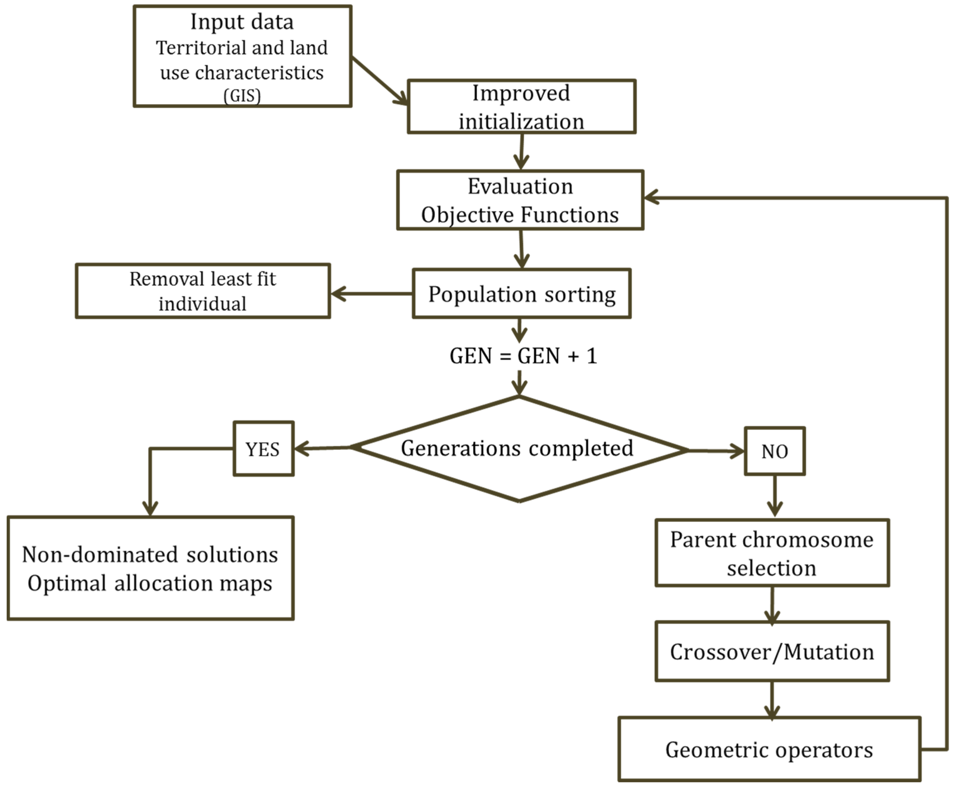
The model for sustainable land use allocation known as MAUSS (Spanish acronym for “Modelo de Asignación de Uso Sostenible de Suelo”) solves the multi-objective optimization problem described above. MAUSS incorporates the multi-objective genetic algorithm NSGA II [31], which has been substantially modified to fit the spatial planning problem stated previously as shown below. A flow chart of the model is shown in Figure 2.
2.3.1. Chromosome Representation
In this work, grid-based representation is used due to both its ease of computing through homogeneous territorial units (squared cells) and its appropriateness for a sub-regional work scale in which plot configuration is irrelevant for the territorial analysis. Thus, as the chromosome is the operational element of any GA, a chromosome or individual comprised of the map grid represents every possible solution of the optimization problem. Every chromosome gene is a map cell.
2.3.2. Initialization
Spatial rationality to quantitatively and qualitatively improve the existing land use allocation is based on two key issues: land use compactness and land required per land use on a case-by-case basis. According to this, an enhanced process to generate the initial population has been designed in order to create rational initial chromosomes that will be improved by the evolutionary process. The initialization process is based on cell agglomeration (patches) per land use type (randomly selected) from a random seed cell or core. Although the concept of seed cell has been used in other works [28], the procedure of this model proves to be more open and expeditious as it does not place restrictions on the number and size of cell patches because they are indirectly and simultaneously controlled by a model parameter called the randomization parameter, whose function is to determine the percentage of random seed cells to be allocated per land use type. Thus, the lower the parameter, the less random seed cells will be allocated and therefore the larger the patch. Patches will expand until the maximum number of cells per land use type is reached. The preliminary considerations for land use allocation in initial chromosomes are as follows:
- (a)
- Random seed cells and their subsequent agglomeration must be allocated in an empty cell within a valid land use subset.
- (b)
- The sum of cells per land use must not exceed the pre-fixed area. Each land use can be allocated in one or several agglomerations depending on the seed randomization parameter.
- (c)
- Only one land use type can be allocated in a cell
The initialization process performs the following steps:
- Random selection of land use allocation order.
- Random selection of seed cells for initiating the agglomeration by allocating the current land use in its eight neighbor cells (3 × 3 cell window). Adjacent cells are then identified (5 × 5 cell window) to act as new seeds until the maximum area per use is reached. All individual cells must accomplish the above considerations.
- Once the current land use cells are completely allocated, the process continues with the next random land use until the chromosome allocates all land uses.
- The initialization process iterates until the initial set of chromosomes (population) is completed.
As a topologic structure, valid subsets per land use in a map can share a portion, none, or their entire dimension with more than one valid subset due to the territorial aptitude for more than one land use type. Therefore, a land use may not reach its prefixed extension because its valid subset can be crowded by other land uses. To overcome this problem, deficit land uses fill the unallocated chromosome cells until they are completed. Suitable allocations will subsequently be improved via genetic operators.
Initialization ensures diversity among individuals and the land use compactness within them so that the evolutionary process can take place.
2.3.3. Model Operators
The MAUSS model operators are classified into genetic and geometric operators according to the following description.
A Genetic operators
Like GAs, crossover and mutation operators perform recombination or reproduction tasks to promote diversity among offspring from which optimal solutions are then obtained.
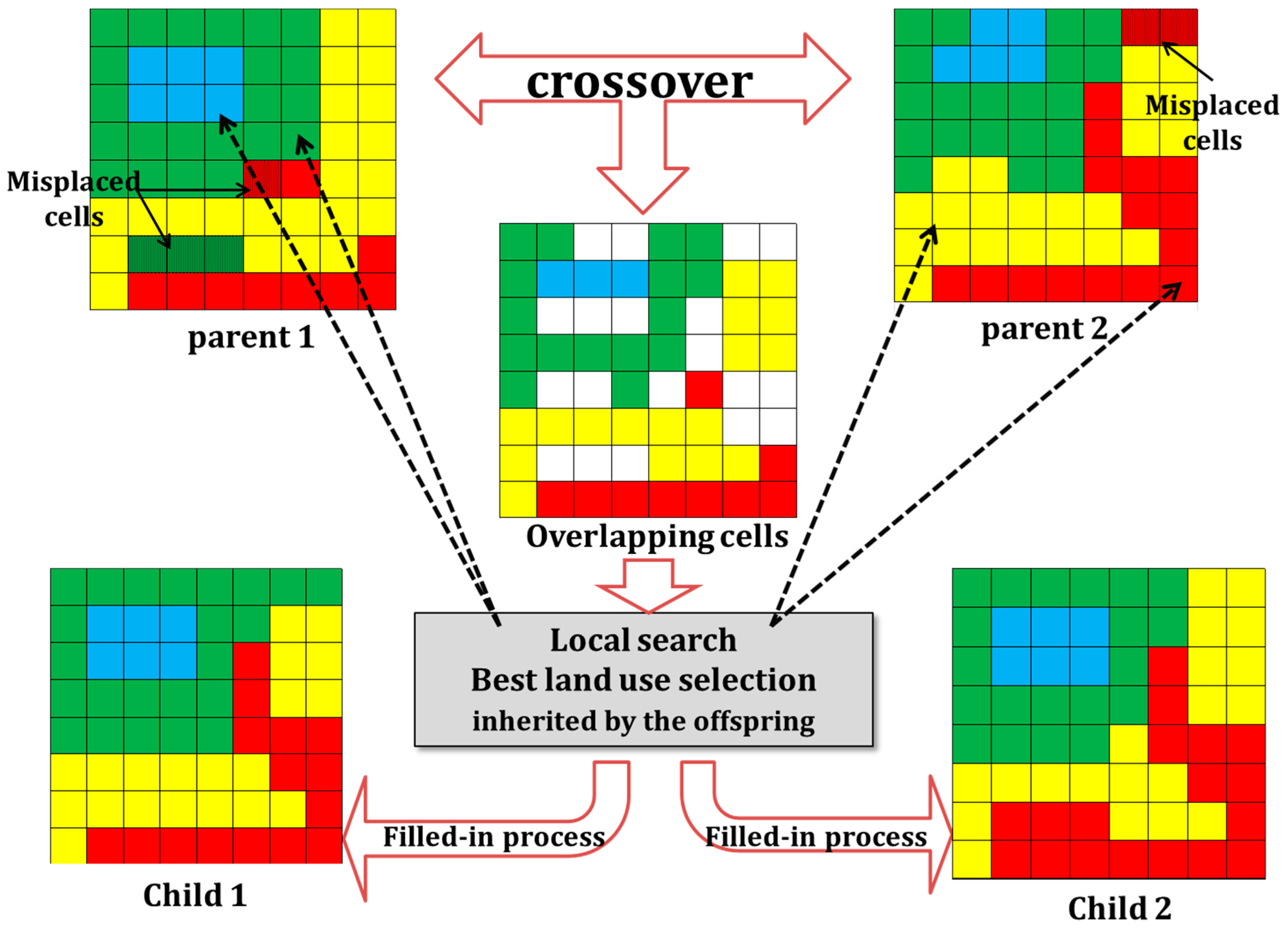
Crossover operator. Traditionally, population reproduction via crossover consists in swapping segments from two chromosomes or parents. These segments, which are defined by a single crossing point or multiple crossing points along the matching chromosomes, generate offspring according to some criteria containing the genetic information of both parents. The NSGA-II crossover operator differs from the aforementioned crossover operator but is insufficient for obtaining rational solutions in spatial optimization problems. Therefore, it has been adapted (see Figure 2) in the present work. Specifically, once a chromosome set for reproduction is defined (half of the total population), a pair of chromosomes (parents) is selected at random with a 90% of probability for crossing as follows:
- (1)
- Overlapping stage: Cells of parent one and parent two in whose positions land use type is equal (overlapped cells) are inherited by child one and child two provided they are located within their valid subsets. Matching cells containing different land uses remain empty.
- (2)
- Local search stage: To fill empty cells, a local search is applied in this work for each land use type by a similar procedure to that proposed by Datta et al. [5]. The objective functions of the model are evaluated in each parent per land use at a time into one minimization function OU (Equation (11)). In contrast to the authors above, the result is not weighted but compared with both parents. The land use with the minimum value is then allocated in the empty cells of child 1 and child 2 alternatively, provided that the above restrictions are accomplished (Equations (6)–(10)). Therefore, the offspring inherits the best land use allocations obtained by the local search and improves global chromosome evaluation.where M is the number of objective functions of the model from j to M; is the value of current land use from i to U evaluated at the jth objective for the (x) parent (parent 1 or parent 2); and and are the maximum and minimum values obtained from the initial population set evaluated for the ith (current) land use U at the jth objective function.
- (3)
- Filled-in stage: The remaining empty cells, which are those outside their valid subset (misplaced), go through a filled-in process similar to the initialization process above. Specifically, the process starts with the random allocation of seed cells (according to the randomization parameter) per deficit land use at least until the lower surface limit for the current land use is reached. This process iterates in descending order beginning from the highest land use deficit (that could be 100 percent). If there is more than one absent land use in the offspring, the iteration process starts with the land use of the smallest extension, provided that restrictions are being accomplished.
The crossing process finishes when there are no empty cells in the offspring.
Mutation operator. This genetic operator aims to relocate land use cells outside their valid subset and therefore diversity among individuals with a mutation probability of 10%, mutation performs as indicated below (Figure 3):
- (1)
- Identifies cells with misplaced land uses.
- (2)
- In a 3 × 3 analysis window, misplaced cells take the most frequent land use in the window if they are exclusively within their valid subsets.
B Geometric operators
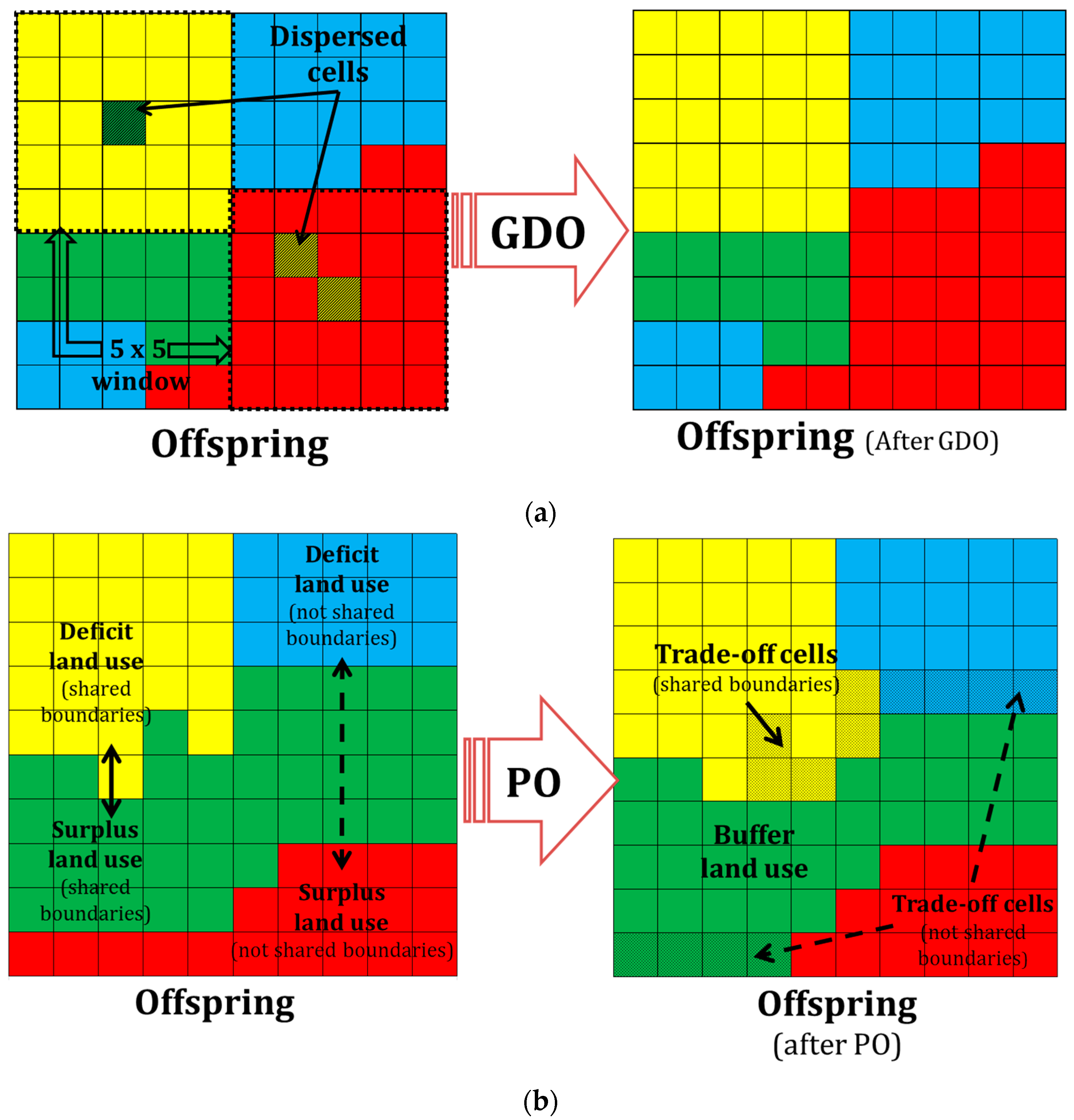
To maintain and improve land use size and compactness, two geometric operators have been developed in this work. As has been widely reported in the literature, in most optimization models of land use allocation, the key elements for improving land use agglomerations in a territory are their boundaries. Thus, a boundary-based analysis is commonly included in spatial models [3,5] because they control the patch size and its compactness, while maintaining the number of required cells per land use. Due to the advantages of the guided initialization of the initial chromosome population, two geometric operators are enabled in this work as correctness mechanisms that perform immediately after the genetic operators in a chromosome for improving territorial rationale through a two-step boundary analysis:
- (1)
- The geographic dispersion operator (GDO) was designed to enhance the compactness of patches. The GDO identifies land use cells allocated either within or outside their feasible subset in a 5 × 5-analysis cell window spread (Figure 4a). Once identified, they turn into the most frequent land use of the neighboring cells. Geographic dispersion must be defined for each implementation of the model because it depends on both geographic extent and cell size, and is related to the specific spatial optimization targets and the available local cartography. In this work, dispersion is understood in the analysis window as one or two maximum adjacent cells whose land use type differs from the remaining neighboring cells. The process iterates until there are no more spread cells in the grid.
- (2)
- The proportion operator (PO) performs by land-use pairs at a time and controls the number of cells required per land use through a patch boundary analysis. Firstly, the operator identifies unbalanced (deficit or surplus) land uses. Each unbalanced land use type can be allocated in one or several cell patches. The land uses with the highest deficit and highest surplus are then chosen. Secondly, the boundary analysis indicates if both uses are neighbors at least in one patch or not. In the first case, the trade-off is immediate only in cells within the constraints; hence the deficit/surplus could be balanced or diminished, but enables the operator to choose a second pair of land uses of unbalanced size using the same criterion as above. This process iterates until all land use sizes are compensated or until there are no neighbors between the remaining unbalanced land uses. In that case, a different land use patch that shares boundaries with a deficit patch enables proportioning by ceding cells which are transformed into the deficit land use type and later compensated by the surplus land use. This operator iterates in two or more patches until map land uses proportion (within the upper and lower limits of pre-fixed areas) is reached, provided that the spatial restrictions are fulfilled (Figure 5b).
After the geometric operators correct the compactness and size of the last child subject to the genetic operators (crossover or mutation), the offspring is evaluated by objective functions and the evolutionary process iterates until all generations are completed (see Figure 1), thus providing the corresponding non-dominated set of solutions.
2.4. Case Study. Application of MAUSS to the Plains of San Juan
Study Area Description
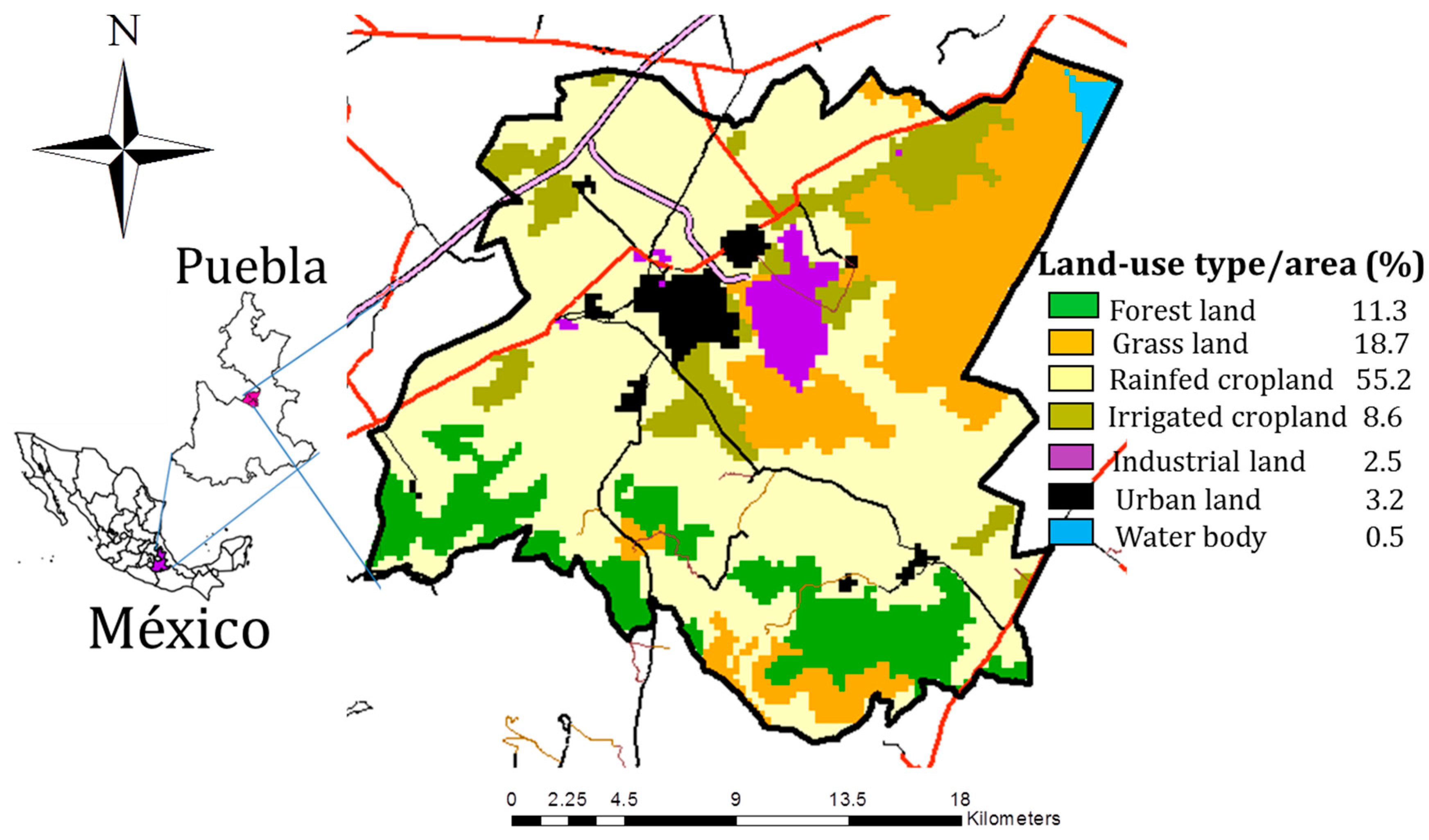
The Plains of San Juan are located in the center of Puebla state (central Mexico) between 19°10′38′′N to 19°16′41′′N latitudes and 97°55′85′′W to 97°37′79′′W longitudes (Figure 6). The area occupies a sub-region of some 500 km2 within the plains, which is undergoing a rapid industrialization process led by the automotive sector. Five municipalities comprise the area, which has 63,770 inhabitants [40] settled in three small urban centers and several rural communities whose overriding productive activity is primary production for self-consumption and local trade. Nonetheless, in the last three years, urban and industrial expansion has spread without effective regulations and most of the significant land use changes have taken place in the sub-region without an official land use plan.
Six land use types have been considered (grouped from the official land use map, scale 1:250,000) [41] with the aim of applying MAUSS to the Plains of San Juan: (1) forest; (2) grassland; (3) rain fed crops; (4) irrigated crops; (5) industrial land; and (6) urban land. The study area is represented in a grid of 111 × 121 squared cells with 250 m per side (Figure 6).
3. Results
After several trial runs, the number of iterations and some of the model parameters were fixed, as is explained below. The model execution starts from an initial population of 150 individuals for 150 generations. Execution time took 12 h in a standard PC (core i5, at 3.1 Ghz).
3.1. Model Parameters
MAUSS was applied assuming some complementary spatial restrictions due to local conditions: (1) areas with consolidated human settlements (urban or rural) and existing water bodies (small intermittent lagoons) were not susceptible to land use change; (2) in steeply sloping areas (more than 15% slope), forestland was preserved; and (3) current irrigated land was also preserved due to the lack of irrigation infrastructure in the study area and its importance to guarantee food production for the population. Prefixed area per land use has a variability range of ±3%, which is the percentage used to establish the upper and lower limits of area for each land use type. All these restrictions were taken into account in the initialization process and affected 18.6% of the total study area.
The model parameters were calibrated as follows. The randomization parameter was set at 3% in both the initialization procedure and the filled-in stage within the cross-over operator. Territorial aptitude factors that affect all objective functions were obtained in qualitative terms (classified into four categories: very high, high, average and low aptitude) from the available cartographic information, and transformed into quantitative values (from 0.5 to 1) on the basis of local agricultural statistics for a 10-year period [42,43]. CO2 emission values [44,45,46] were weighted by the accessibility index defined above, which varies between 1 (toll road) and 0.25 (local road) according to the distance of each cell to the closest communication link and its hierarchy. Water demands in the Plains of San Juan are satisfied from groundwater withdrawals, thus potential pollutant risk was only evaluated for groundwater. The conversion factor for transforming crops into alimentary units (calories) was calculated for each of the 23 main crops of the region pursuant to the USDA nutrients database [47]. A healthy diet was defined as 2500 kilocalories per person according to the WHO [48].
3.2. Evolutive Performance
3.2.1. Global Improvements
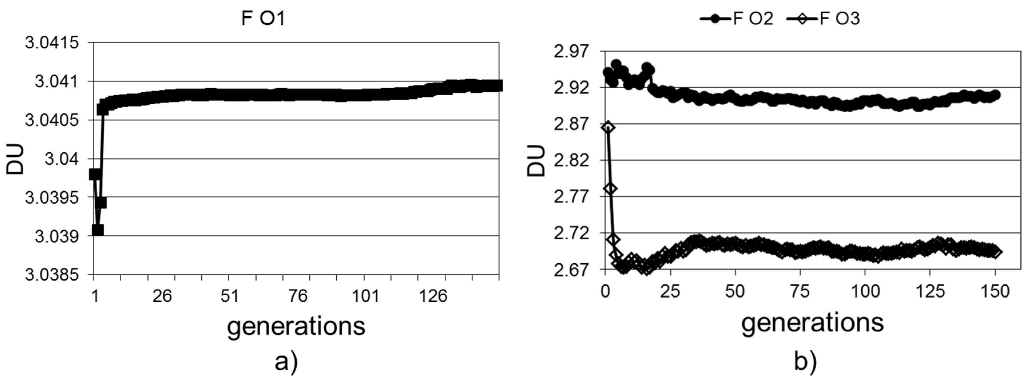
Figure 7 shows the performance of each objective function with average values over the generations. Substantial improvements were achieved in the first ten iterations in each objective until the values became stable. The evolutionary process improved all values of the initial set of chromosomes.
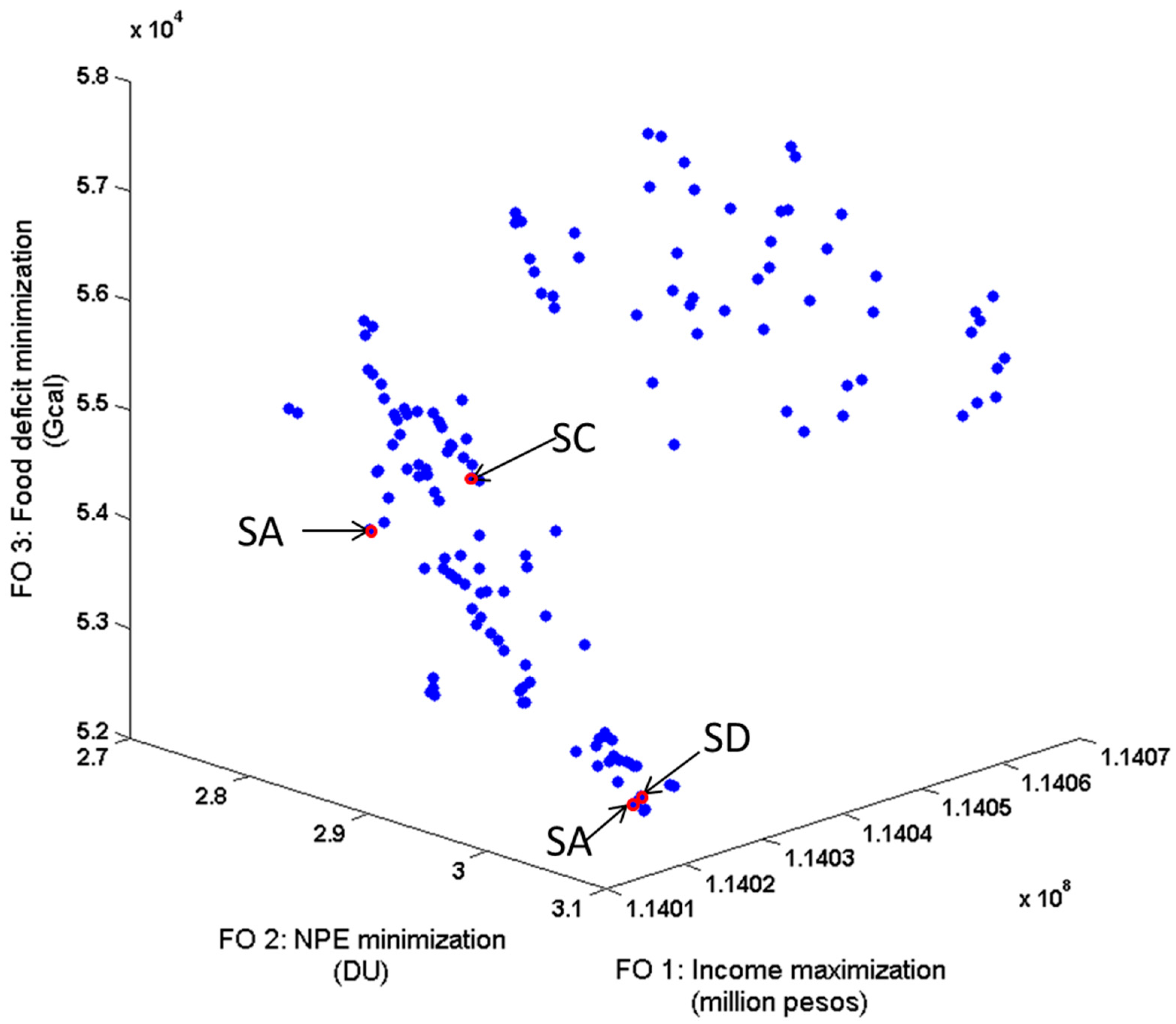
Figure 8 shows the set of non-dominated solutions obtained after 150 generations. It includes selected solutions as will be explained below.
3.2.2. Improvements per Land Use Type
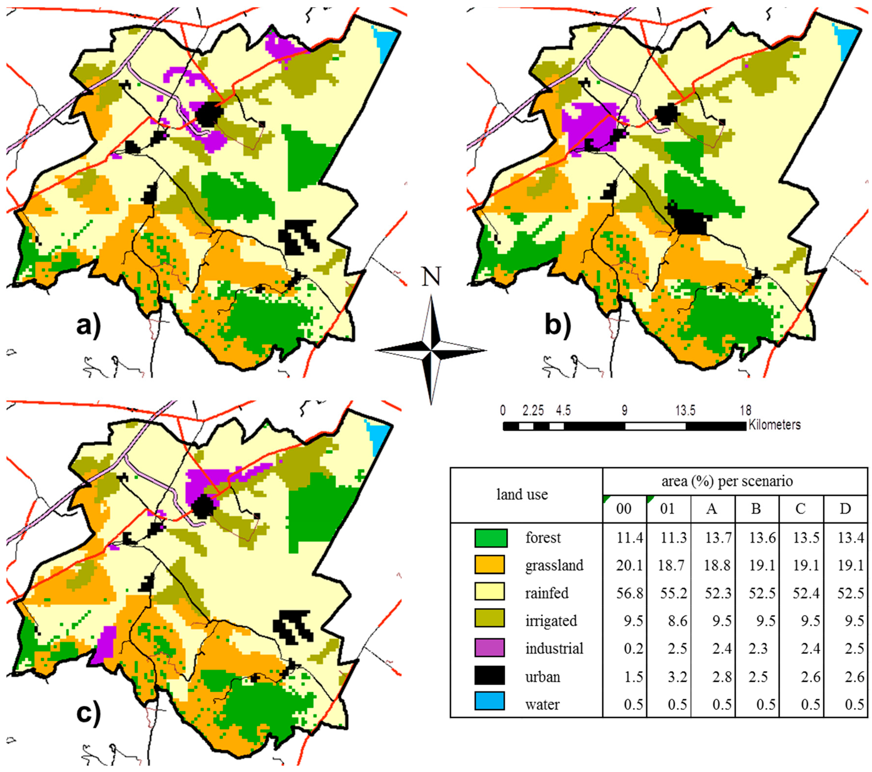
The results are presented in several scenarios to clarify the huge territorial transformations ongoing and the land use allocation improvements using the MAUSS model: Scenario 00 (S00), land use distribution before the industrial expansion of automotive sector; Scenario 01 (S01), current land use allocation (official proposal) and Optimal Scenarios (A, B, C and D), defined by both the solutions selected from the non-dominated set of solutions after the evolutionary process. The definition of optimal scenarios is based on both the level of accomplishment of the objective functions: the best solutions for functions O1 (scenario A [SA]), O2 (scenario B [SB]), O3 (scenario C [SC]) and the trade-off solution (scenario D [SD]); and the most suitable land-use distribution. The fixed values of the cells not considered in the evolutionary process due to the restrictions explained above were added to the results of evolved solutions in order to establish comparable scenarios. Due to the nature of the spatial planning problem, a simple criterion to select scenarios has been considered instead of more sophisticated procedures like the knee method [49,50]. MAUSS aims to provide reference solutions to set the study region within the non-dominated set of solutions and aid spatial planners in decision-making processes, which are strongly affected by other factors (e.g., cadastral borders and land ownership) that cannot be incorporated in the mathematical approach of the problem.
The analysis scenarios are highlighted in Figure 8 and concentrated in the region with highest dot density.
• Income Maximization
Average annual gross income per land use was estimated from national and regional databases [42,43] for the different scenarios. As shown in Table 1, the sub-regional income initially increases by more than 22 times for industrial and urban settlements (from 5174.93 pesos in S00 to 118,837.27 million pesos in S01). In all optimal scenarios, annual incomes were higher than in S01. For SA (best individual for F O1), the income is 607.3 million pesos higher than S01 (119,444.6 million pesos). The results of income per land use show that the most significant monetary increases from S01 to the optimal scenarios (SA, SB, SC, and SD) are due in all cases to grassland use, whereas for SA it is also due to industrial land use. Grassland area is slightly larger (Figure 7) in the optimal scenarios than in S01 but lower than in S00. Nonetheless, the income for the optimal scenarios is about 63% and 54% higher than in S01 and S00, respectively. The optimal scenarios maintained the same annual income of irrigated land since its location and area remain unchanged from scenario 00, according to the additional constraints specified above.
• Minimization of negative pressures on the environment
Table 2 shows the negative pressures expressed in dimensionless units according to Section 2.1 that each land use type exerts on the environment (water and air). The expansion of industrial and urban land uses considerably increases the NPE in the sub-region (from 3.151 in S00 to more than 3.4 in all other scenarios). In SA, SB, SC, and SD, pressures on the environment were always lower (around 9%) than for the actual land use distribution (S01). The best individual for F O2 (SB) yielded a minimum value of 3.482 and reached lower pressures precisely in industrial and urban land uses.
• Minimization of food deficit
As shown in Table 3, the study area is currently a food surplus region (negative deficit). However, the loss of food-producing land decreased the nourishment surplus at the sub-regional scale from 193.64 AU in Gigacalories (Gcal) in S00 to 182.67 in S01. SC yielded a lower food surplus of 173.19 Mcal, which is 5.2% and 10.6% lower than S01 and S00, respectively. The analysis of land use showed that, even in the optimal scenarios, the grassland area decreased from S00 and slightly increased from S01 (see Figure 6), while the alimentary values increased to 2.96 in SC, representing a 53% and 64% increase over S00 and S01, respectively. No significant global Gcal increases were observed, while significant alimentary decreases were due to the reduction in rainfed cropland area.
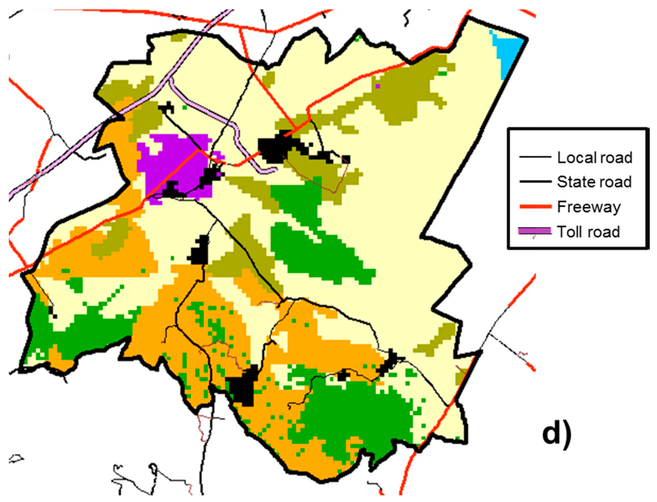
• Best solution maps
Geographical representation of best individuals selected for each scenario is shown in Figure 9. Scenario D is the solution map that best achieves the three objective functions. Compared to S01, its income is 17.4 million pesos (1.5%) higher, its global NPE is 9.4% lower and its food deficit is 6.9 Gcal lower (a reduction of 3.76%). The NPE for urban, grassland and industrial land uses is significantly lower than S01 (24.7%, 16.7%, and 3.5%, respectively).
4. Discussion
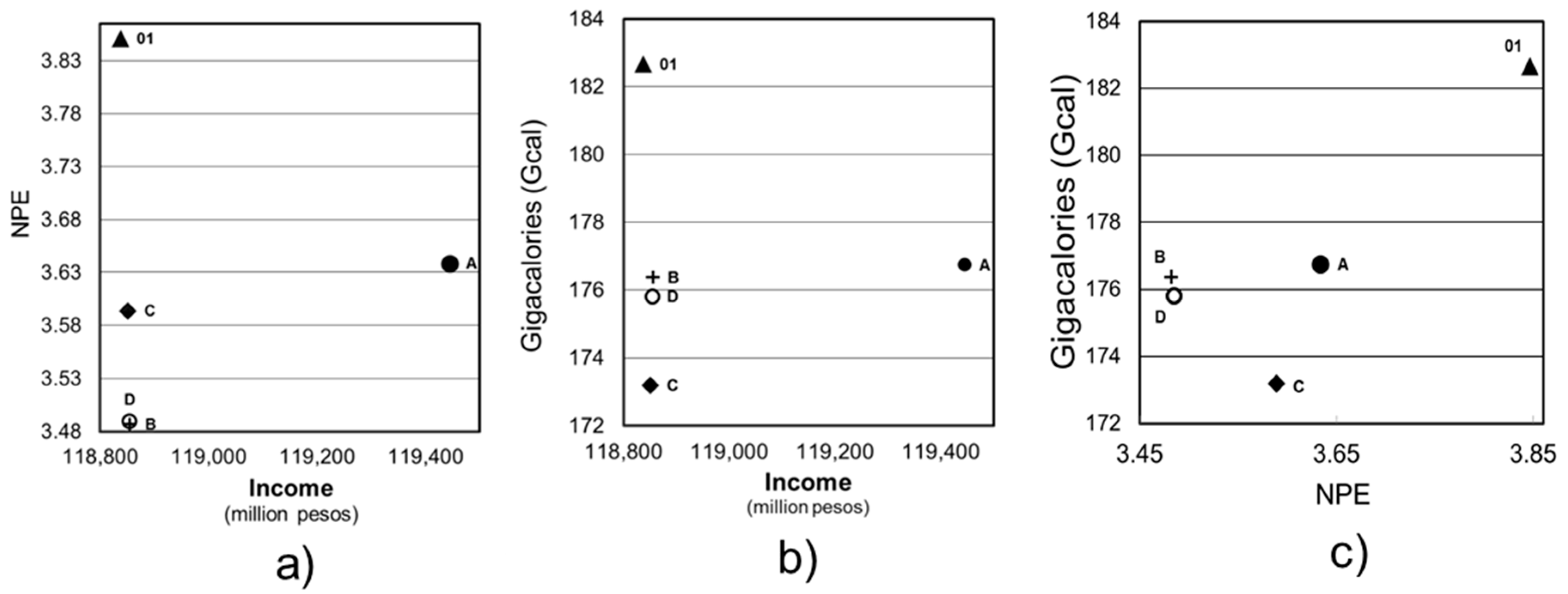
In order to show the effectiveness of MAUSS, the optimal scenarios (SA, SB, SC, and SD) and the official proposal (S01) are located in the bi-dimensional solution space (Figure 10). As can be seen, the best individuals extracted from the non-dominated set of solutions obtained better evaluations in each of the three objective functions, as described above.
The effectiveness of MAUSS can be observed in the way in which it solves the multi-objective problem. For example, to increase income, the model produced small increases in the size of certain land uses (i.e., industrial and urban land uses in SA) taking into account the established restrictions. These small variations in size resulted in large increases in income. The model also allocated grasslands to areas with a greater aptitude whose higher income did not significantly increase the sum of calories or the negative pressure on the environment. Additionally, in order to minimize NPE, urban and industrial land uses were allocated next to main roads (to decrease CO2 emissions) and in areas with a lower polluting potential of groundwater, which not only preserved but also increased forestland. To minimize food deficit, the MAUSS model worked in two ways: (a) it preferred rainfed land allocations to satisfy the new requirements of urban and industrial land uses; and (b) it gave priority to grasslands over rainfed land, thus preventing significant increases in crop production and a higher WF.
For S01, around 2200 ha of land were required for industrial and urban development in the study area, which was achieved by occupying irrigated lands, grasslands and rainfed lands, whose surface loss is 9.6%, 7.0%, and 3.0%, respectively. In optimal scenarios, such land use changes were established at 1850 ha from grassland and rainfed lands (with a loss of 5% and 8%, respectively). As described, the irrigated cropland area remained unchanged due to the lack of irrigation infrastructure in the region and its importance for future food production needs. For an expected population of 250,000 inhabitants by the year 2030, S01 considered a very large area per person of 67 m2, which significantly increases negative pressures on the environment.
Future lines of research should be aimed at evaluating landscape transformations in the medium and long term under certain development conditions (i.e., population growth, variations in investment rate, agricultural improvements, etc.); refining the polluting risk indicator for surface water, from a spatial planning approach; and including methodologies to determine the carrying capacity of a territory in which the maximum usage of its resources is limited.
MAUSS is a powerful tool that may help planners to make decisions in regions with a high probability of undergoing extreme land use changes as it provides sustainable landscapes.
5. Conclusions
The MAUSS model incorporates the sustainability concept for spatial planning using three objective functions (maximizing income, minimizing negative pressure on environment and minimizing food deficit) at sub-regional scale. In territories with problems of famine but also in those where food needs are met, it is important to emphasize the inclusion of food goals in an objective function in order to reduce unnecessary food imports as well as environmental degradation. An objective function of this type would reduce the per capita ecological footprint and improve regional sustainability, contributing in turn to global sustainability.
The model exploits the ability of a multi-objective evolutionary algorithm to perform a detailed evaluation of relevant territorial aspects using several objective functions rather than oversimplifying spatial analysis to a single aptitude or fitness function. It also incorporates new geometric operators to preserve spatial rationality and a new initialization procedure. All of these features facilitate the solution of the sustainable spatial planning problem stated in this paper.
The model has been successfully applied to the Plains of San Juan, a sub-region located in central Mexico. The MAUSS solutions, drawn from the non-dominated set of solutions, increase income by up to 1% compared to the current income. In relation to the negative pressures exerted on water (water footprint and pollution potential) and air (CO2 equivalent emissions), these solutions achieve a global reduction of 9%, as well as the possibility of averting potential risks of water resources, which are usually considered separately from spatial planning goals. The model also reduces CO2 equivalent emissions by enhancing the accessibility and compactness of urban and industrial land uses and deterring land use changes in order to diminish fossil fuel usage in a land use configuration. As regards the alimentary goals in the Plains of San Juan, MAUSS reduces the food surplus by 5.2% by allocating agricultural land to more profitable uses while maintaining food security in the region.
For further details about the cartographic and data inputs for objective functions, see the supplementary materials section.
Supplementary Materials
The following supplementary materials are available online at www.mdpi.com/2071-1050/9/6/927/s1, Figure A1: Map of ground water vulnerability (V) according to DRASTIC, Figure A2: (a) Map of distances to closest communication link; and (b) map of accessibility index, Table A1: Input data for F O3, Table A2: Aptitude factors per land use type, Table A3: Input data per surface units (Ha) for F O2.
Acknowledgments
The authors would like to thank the National Council of Science and Technology (CONACyT), Mexico, for financing and making this research possible under grant CVU546486. Special thanks to the Iberoamerican University Association for Postgraduate Studies (AUIP) for of its international programs of scientific cooperation between Spain and Iberoamerica and granting mobility support to doctoral students.
Author Contributions
Guadalupe Azuara García made substantial contributions to the design of the study, participated in the analysis and the interpretation of data, and drafted the manuscript. Efrén Palacios Rosas programmed the model into MATLAB language. Alfonso García-Ferrer supervised all cartographic pre-processing. Pilar Montesinos Barrios participated in the design of the study and supervised all methodologies utilized for the construction of the model. All authors read and approved the final manuscript.
Conflicts of Interest
The authors declare no conflict of interest.
References
- Laurance, W.F.; Cochrane, M.A.; Bergen, S.; Fearnside, P.M.; Delamônica, P.; Barber, C.; D’Angelo, S.; Fernandes, T. The Future of the Brazilian Amazon. Science 2001, 291, 438–439. [Google Scholar] [CrossRef] [PubMed]
- United Nations Environmentl Programme. Online Version of the Article. The Disappearance of the Aral Sea. Vital Water Graphics, an Overwiew’ of the State of the World’s Fresh and Marine Waters, 2nd ed. 2002. Available online: http://wedocs.unep.org/handle/20.500.11822/20624 (accessed on 9 May 2017).
- Cao, K.; Batty, M.; Huang, B.; Liu, Y.; Yu, L.; Chen, J. Spatial multi-objective land use optimization: Extensions to the non-dominated sorting genetic algorithm-II. Int. J. Geogr. Inf. Sci. 2011, 25, 1–21. [Google Scholar] [CrossRef]
- Stewart, T.; Janssen, R.; Herwijnen, M. A genetic algorithm approach to multiobjective land use planning. Comput. Oper. Res. 2004, 31, 2293–2313. [Google Scholar] [CrossRef]
- Datta, D.; Deb, K.; Fonseca, C.; Lobo, F.; Condado, P. Multi-Objective Evolutionary Algorithm for Land-Use Management Problem. Int. J. Comput. Intell. Res. 2006, 3, 1–24. [Google Scholar]
- Karakostas, S. Multi-objective optimization in spatial planning: Improving the effectiveness of multi-objective evolutionary algorithms (non-dominated sorting genetic algorithm II). Eng. Optim. 2015, 47, 601–621. [Google Scholar] [CrossRef]
- Liu, X.; Ou, J.; Li, X.; Ai, B. Combining system dynamics and hybrid particle swarm optimization for land use allocation. Ecol. Model. 2013, 257, 11–24. [Google Scholar] [CrossRef]
- Jalem, K. Development of water resources for micro watershed at Chinamushidiwada Village in Visakhapatnam, Andhra Pradesh, India. J. Civ. Environ. Eng. 2016. [Google Scholar] [CrossRef]
- Food and Agriculture Organization. Conceptualizing the linkages, Commodity Policy and Projections Service. In Trade Reforms and Food Security; Commodities and Trade Division: Rome, Italy, 2003; Part 1, Chapter 2; pp. 25–34. [Google Scholar]
- Zhang, H.; Zeng, H.; Jin, X.; Shu, B.; Zhou, Y. Simulating multi-objective land use optimization allocation using Multi-agent system—A case study in Changsha, China. Ecol. Model. 2016, 320, 334–347. [Google Scholar] [CrossRef]
- Liu, Y.; Tang, W.; He, J.; Liu, Y.; Ai, T.; Liu, D. A land-use spatial optimization model based on genetic optimization and game theory. Comput. Environ. Urban Syst. 2015, 49, 1–14. [Google Scholar] [CrossRef]
- Schlager, K.J. A land use plan design model. J. Am. Plan. Assoc. 1965, 31, 103–111. [Google Scholar] [CrossRef]
- Chuvieco, E. Integration of linear programming and GIS for land-use modelling. Int. J. Geogr. Inf. Sci. 1993, 7, 71–83. [Google Scholar] [CrossRef]
- Arthur, J.; Nalle, D. Clarification on the use of linear programming and GIS for land-use modelling. Int. J. Geogr. Inf. Sci. 1997, 11, 397–402. [Google Scholar] [CrossRef]
- Malczewski, J. GIS and Multicriteria Decision Analysis; Wiley: New York, NY, USA, 1999. [Google Scholar]
- Balling R, J.; Brown, M.R.; Day, K. Multiobjective urban planning using genetic algorithm. J. Urban Plan. Dev. 1999, 125, 86–99. [Google Scholar] [CrossRef]
- Fernández, I.; Rodríguez, J.A.; Camacho, E.; Montesinos, P. Optimal Operation of Pressurized Irrigation Networks with Several Supply Sources. Water Resour. Manag. 2013, 27, 2855–2869. [Google Scholar] [CrossRef]
- Fernández, I.; Montesinos, P.; Camacho, E.; Rodríguez, J.A. Methodology for detecting critical points in pressurized irrigation networks with multiple water supply points. Water Resour. Manag. 2014, 28, 1095–1109. [Google Scholar]
- Delgado-Osuna, J.A.; Lozano, M.; García-Martínez, C. An alternative artificial bee colony algorithm with destructive–constructive neighbourhood operator for the problem of composing medical crews. Inf. Sci. 2016, 326, 215–226. [Google Scholar] [CrossRef]
- Goldberg, D.E. Genetic Algorithms in Search, Optimization and Machine Learning; Addison Wesley Longman: Boston, MA, USA, 1989. [Google Scholar]
- Ma, X.; Zhao, X. Land use allocation based on a multi-objective artificial immune optimization model: An application in Anlu County, China. Sustainability 2015, 7, 15632–15651. [Google Scholar] [CrossRef]
- Huang, K.; Liu, X.; Li, X.; Liang, J.; He, S. An improved artificial immune system for seeking the Pareto front of land-use allocation problem in large areas. Int. J. Geogr. Inf. Sci. 2012, 27, 922–946. [Google Scholar] [CrossRef]
- Liu, X.P.; Li, X.; Shi, X. A multi-type ant colony optimization (MACO) method for optimal land use allocation in large areas. Int. J. Geogr. Inf. Sci. 2012, 26, 1325–1343. [Google Scholar] [CrossRef]
- Dorigo, M.; Blum, C. Ant colony optimization theory: A survey. Theor. Comput. Sci. 2005, 344, 243–278. [Google Scholar] [CrossRef]
- Mathews, K.B.; Sibald, A.; Craw, S. Implementation of a spatial decision support system for rural land use planning: Integrating geographic system and environmental models with search and optimization algorithms. Comput. Electron. Agric. 1999, 23, 9–26. [Google Scholar] [CrossRef]
- Feng, C.M.; Lin, J.J. Using a genetic algorithm to generate alternative sketch maps for urban planning. Comput. Environ. Urban Syst. 1999, 23, 91–108. [Google Scholar] [CrossRef]
- Buzai, G.D. Análisis Espacial con Sistemas de Información Geográfica: Sus cinco Conceptos Fundamentales. In Geografía y Sistemas de Información Geográfica. Aspectos Conceptuales y Aplicaciones; Buzai, G.D., Ed.; Universidad Nacional de Luján—GESIG: Luján, Argentina, 2010; pp. 163–195. Available online: http://www.gesig-proeg.com.ar/documentos/articulos/2010-BUZAI-CAP7.pdf (accessed on October 24 2016).
- Stewart, T.; Janssen, R. A multiobjective GIS-based land use planning algorithm. Comput. Environ. Urban Syst. 2014, 46, 25–34. [Google Scholar] [CrossRef]
- Porta, J.; Parapar, J.; Doallo, R.; Rivera, F.; Santé, I.; Crecente, R. High performance genetic algorithm for land use planning. Comput. Environ. Urban Syst. 2013, 37, 45–58. [Google Scholar] [CrossRef]
- Cao, K.; Huang, B.; Wang, S.; Lin, H. Sustainable land use optimization Boundary-based Fast Genetic Algorithm. Comput. Environ. Urban Syst. 2012, 36, 257–269. [Google Scholar] [CrossRef]
- Deb, K.; Pratap, A.; Agarwal, S.; Meyarivan, T. A Fast and Elitist Multiobjective Genetic Algorithm: NSGA-II. IEEE Trans. Evolut. Comput. 2002, 6, 182–197. [Google Scholar] [CrossRef]
- Hoekstra, A.Y.; Chapagain, A.K.; Aldaya, M.M.; Mekonnen, M.M. The Water Footprint Assessment Manual. Setting the Global Standard; Earthscan: London, UK, 2011. [Google Scholar]
- Allen, R.G.; Pereira, L.S.; Raes, D.; Smith, M. Crop Evapotranspiration—Guidelines for Computing Crop Water Requirements—FAO Irrigation and Drainage Paper 56 (Spanish Version); FAO: Rome, Italy, 2006. [Google Scholar]
- García, J.; Rodríguez, J.A.; Camacho, E.; Montesinos, P. Linking water footprint with irrigation management in high value crops. Implications on sustainable irrigation agriculture in environmentally sensitive areas. J. Clean. Prod. 2015, 87, 594–602. [Google Scholar] [CrossRef]
- González, R.; Camacho, E.; Montesinos, P.; García, J.; Rodríguez, J.A. Influence of spatio temporal scales in crop water footprinting and water use management: Evidences from sugar beet production in Northern Spain. J. Clean. Prod. 2016, 139, 1485–1495. [Google Scholar] [CrossRef]
- Montesinos, P.; Camacho, E.; Campos, B.; Rodríguez, J.A. Analysis of virtual irrigation water. Application to water resources management in a Mediterranean river basin. Water Resour. Manag. 2011, 25, 1635–1651. [Google Scholar] [CrossRef]
- Dávila, R. Desarrollo Sostenible de Usos de Suelo en Ciudades en Crecimiento, Aplicando Hidrogeología Urbana Como Parámetro de Planificación Territorial: Caso de Estudio Linares N.L. México. Ph.D. Thesis, Fac. Ciencias de la Tierra, University Autónoma de Nuevo León, Nuevo León, Mexico, 2011. [Google Scholar]
- Aller, L.; Bennet, T.; Lehr, J.; Petty, R.; Hackett, G. DRASTIC: A Standarized System for Evaluating Ground Water Pollution Potential Using Hydrological Settings; Research Report EPA/600/2-87/035; Environmental Protection Agency (EPA) Research Laboratory: Ada, OK, USA, 1987. Available online: http://nepis.epa.gov/Exe/ZyPDF.cgi/20007KU4.PDF?Dockey=20007KU4.PDF (accessed on 17 October 2015).
- Menconi, M.; Stella, G.; Grohmann, D. Revisting the food component of ecological footprint indicator for autonomous rural settlement models in Central Italy. Ecol. Indic. 2013, 34, 580–589. [Google Scholar] [CrossRef]
- INEGI. Population Census; INEGI: Mexico City, Mexico, 2010.
- UNAM, INEGI. Inventario Forestal Nacional (National Forestry Inventory) Scale 1:250,000; UNAM, INEGI: Mexico City, Mexico, 2000.
- INEGI. Economic Census; INEGI: Mexico City, Mexico, 2014.
- Méx: SAGARPA; SIAP. Agricultural System Information, (2015) Agricultural Database Years 2004–2014, México. Available online: http://www.gob.mx/siap/acciones-y-programas/produccion-agricola-33119?idiom=es (accessed on 3 March 2015).
- Méx: INEEC, 2013 Inventario Nacional de Emisiones GEI (National Inventory of GHG Emissions). Available online: http://www.inecc.gob.mx/descargas/cclimatico/2015_inv_nal_emis_gei.pdf (accessed on 25 October 2015).
- Méx: SEMARNAT. Programa de Gestión de la Calidad del Aire del Estado de Puebla 2012–2020. 2012. Available online: http://www.semarnat.gob.mx/archivosanteriores/temas/gestionambiental/calidaddelaire/Documents/ProAire%20Puebla2.pdf (accessed on 20 August 2015).
- Audi. Corporate Responsibility Report 2014; Audi AG: Ingolstadt, Germany, 2014; Available online: http://www.audi.com/content/dam/com/EN/corporate-responsibility/audi_cr_report_2014_en.pdf (accessed on 20 May 2016).
- USDA National Nutrient Database for Standard Reference. Available online: https://www.ars.usda.gov/northeast-area/beltsville-md/beltsville-human-nutrition-research-center/nutrient-data-laboratory/docs/usda-national-nutrient-database-for-standard-reference/ (accessed on 10 February 2016).
- WHO: World Health Organization. Estudio Sobre la Necesidad de una Regulación Económica Más Estricta Para Revertir la Epidemia de la Obesidad. BOLETÍN de la Organización Mundial de la Salud. February 2014. Available online: http://www.who.int/bulletin/releases/NFM0214/es/ (accessed on 8 September 2016).
- Nandi, A.K.; Chakraborty, D.; Vaz, W. Design of a comfortable optimal driving strategy for electric vehicles using multi-objective optimization. J. Power Source 2015, 283, 1–18. [Google Scholar] [CrossRef]
- Branke, J.; Deb, K.; Dielrof, H.; Osswald, M. Finding Knees in Multi-Objective Optimization; KanGAL Report Number 2004010; Springer: Berlin/Heidelberg, Germany, 2004. [Google Scholar]
Figure 1.
Territorial discretization.

Figure 2.
Flow chart of the land use optimization process coupling MAUSS and NSGA-II.

Figure 3.
Illustration of MAUSS crossover operator.

Figure 4.
Illustration of MAUSS mutation operator.
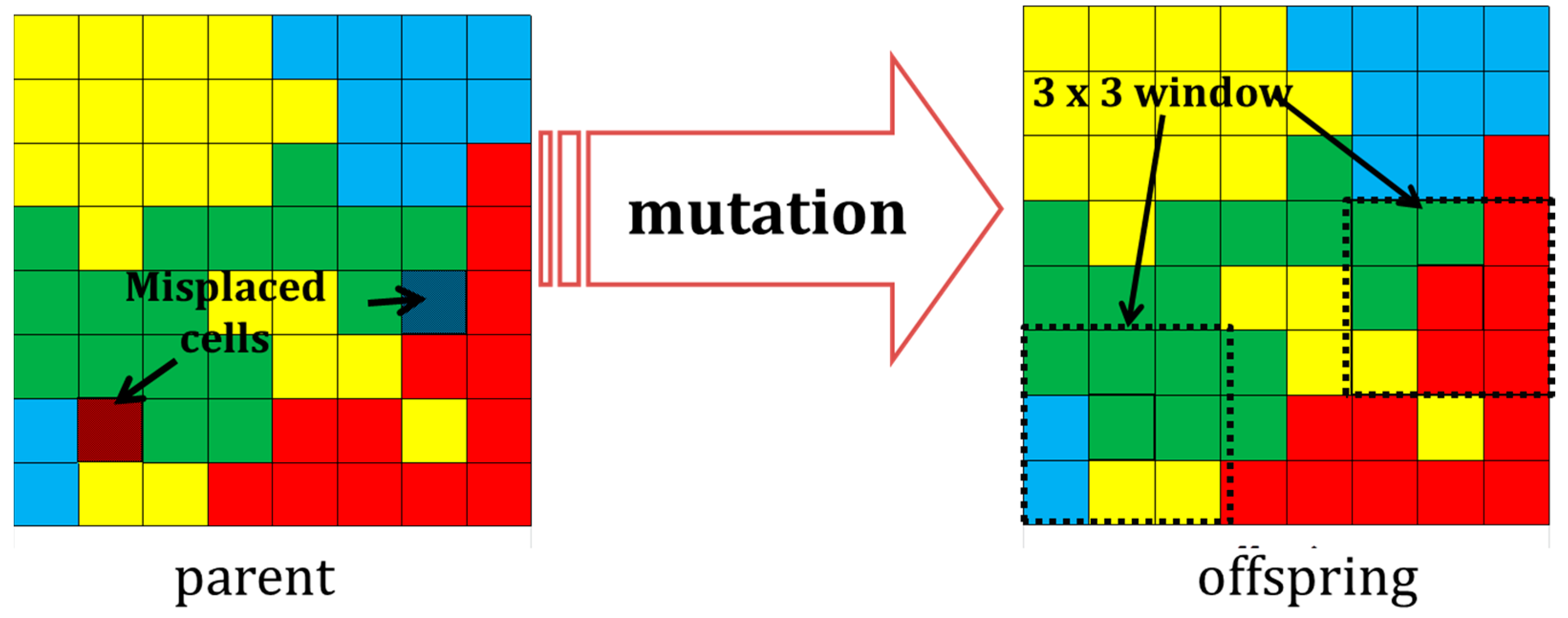
Figure 5.
Illustration of MAUSS geometric operators: (a) geographic dispersion operator (GDO); and (b) proportion operator (PO).
Figure 5.
Illustration of MAUSS geometric operators: (a) geographic dispersion operator (GDO); and (b) proportion operator (PO).

Figure 6.
Current land use allocation in study area (scenario 01).

Figure 7.
Performance of objective functions over generations (mean values per iteration): (a) F O1 Income maximization; and (b) F O2 Minimization of negative pressure on the environment (NPE) and F O3 Minimization of food deficit.
Figure 7.
Performance of objective functions over generations (mean values per iteration): (a) F O1 Income maximization; and (b) F O2 Minimization of negative pressure on the environment (NPE) and F O3 Minimization of food deficit.

Figure 8.
Tridimensional representation of the set of non-dominated solutions after 150 MAUSS generations.
Figure 8.
Tridimensional representation of the set of non-dominated solutions after 150 MAUSS generations.

Figure 9.
Best map solutions per scenario: (a) income maximization (SA); (b) minimization of negative environmental pressure (SB); (c) minimization of food deficit (SC); and (d) trade-off solution (SD).
Figure 9.
Best map solutions per scenario: (a) income maximization (SA); (b) minimization of negative environmental pressure (SB); (c) minimization of food deficit (SC); and (d) trade-off solution (SD).


Figure 10.
Objective function values of scenarios SA, SB, SC, SD (Non-dominated set of solutions) vs. scenario 01 (official proposal): (a) income versus negative pressure on the environment (NPE); (b) income versus food surplus in Gigacalories (Gcal); and (c) negative pressure on the environment (NPE) versus food surplus.


Table 1.
F O1: Annual Income.
| Land Use | Income per Hectare (Million Pesos) | Annual Income Scenario 00 | Annual Income Scenario 01 | Annual Income | |||
|---|---|---|---|---|---|---|---|
| Scenario A | Scenario B | Scenario C | Scenario D | ||||
| forest | 0.00 | 0.00 | 0.00 | 0.00 | 0.00 | 0.00 | 0.00 |
| grassland | 0.03 | 217.68 | 205.60 | 332.43 | 338.83 | 338.15 | 338.73 |
| rain fed cropland | 0.01 | 147.67 | 143.24 | 128.14 | 127.67 | 124.22 | 127.06 |
| irrigated cropland | 0.02 | 41.03 | 37.23 | 41.19 | 41.19 | 41.19 | 41.19 |
| industrial | 70.82 | 4545.27 | 117,962.90 | 118,516.26 | 117,962.90 | 117,962.90 | 117,962.90 |
| urban | 0.29 | 223.27 | 488.30 | 426.58 | 384.83 | 384.25 | 384.83 |
| total | 5174.93 | 118,837.27 | 119,444.60 | 118,855.42 | 118,850.71 | 118,854.71 | |
Table 2.
F O2: Annual values of negative pressure on the environment in dimensionless units.
| Land Use | NPE Scenario 00 | NPE Scenario 01 | NPE | |||
|---|---|---|---|---|---|---|
| Scenario A | Scenario B | Scenario C | Scenario D | |||
| forest | 0.0884 | 0.0884 | 0.0898 | 0.0876 | 0.0877 | 0.0876 |
| grassland | 0.6572 | 0.6075 | 0.5032 | 0.5094 | 0.5102 | 0.5095 |
| rain fed cropland | 1.1049 | 1.0664 | 1.0585 | 1.0724 | 1.0836 | 1.0743 |
| irrigated cropland | 0.0781 | 0.0707 | 0.0781 | 0.0781 | 0.0781 | 0.0781 |
| industrial | 0.7940 | 1.0354 | 0.9985 | 0.9982 | 1.0039 | 0.9985 |
| urban | 0.4282 | 0.9782 | 0.9057 | 0.7364 | 0.8255 | 0.7369 |
| total | 3.151 | 3.847 | 3.634 | 3.482 | 3.589 | 3.485 |
Table 3.
F O3: Food surplus. Gigacalories (Gcal) for agricultural land uses.
| Land Use | Food Surplus Scenario 00 | Food Surplus Scenario 01 | Food Surplus Optimal Scenarios | |||
|---|---|---|---|---|---|---|
| Scenario A | Scenario B | Scenario C | Scenario D | |||
| grassland | 1.93 | 1.80 | 2.92 | 2.98 | 2.96 | 2.97 |
| rain fed cropland | 120.88 | 115.75 | 103.76 | 103.35 | 100.34 | 102.82 |
| irrigated cropland | 70.83 | 65.12 | 70.06 | 70.04 | 69.89 | 70.02 |
| total | 193.64 | 182.67 | 176.74 | 176.37 | 173.19 | 175.81 |
© 2017 by the authors. Licensee MDPI, Basel, Switzerland. This article is an open access article distributed under the terms and conditions of the Creative Commons Attribution (CC BY) license (http://creativecommons.org/licenses/by/4.0/).
Share and Cite
MDPI and ACS Style
García, G.A.; Rosas, E.P.; García-Ferrer, A.; Barrios, P.M. Multi-Objective Spatial Optimization: Sustainable Land Use Allocation at Sub-Regional Scale. Sustainability 2017, 9, 927. https://doi.org/10.3390/su9060927
AMA Style
García GA, Rosas EP, García-Ferrer A, Barrios PM. Multi-Objective Spatial Optimization: Sustainable Land Use Allocation at Sub-Regional Scale. Sustainability. 2017; 9(6):927. https://doi.org/10.3390/su9060927
Chicago/Turabian StyleGarcía, Guadalupe Azuara, Efrén Palacios Rosas, Alfonso García-Ferrer, and Pilar Montesinos Barrios. 2017. "Multi-Objective Spatial Optimization: Sustainable Land Use Allocation at Sub-Regional Scale" Sustainability 9, no. 6: 927. https://doi.org/10.3390/su9060927
Note that from the first issue of 2016, this journal uses article numbers instead of page numbers. See further details here.