A Joint Evaluation of the Wind and Wave Energy Resources Close to the Greek Islands


Department of Mechanical Engineering, Faculty of Engineering, “Dunărea de Jos” University of Galati, 47 Domneasca Street, Galati 800008, Romania
*
Author to whom correspondence should be addressed.
Sustainability 2017, 9(6), 1025; https://doi.org/10.3390/su9061025
Submission received: 28 April 2017
/
Revised: 5 June 2017
/
Accepted: 7 June 2017
/
Published: 15 June 2017
(This article belongs to the Special Issue Wind Energy, Load and Price Forecasting towards Sustainability)
Abstract
:The objective of this work is to analyze the wind and wave energy potential in the proximity of the Greek islands. Thus, by evaluating the synergy between wind and waves, a more comprehensive picture of the renewable energy resources in the target area is provided. In this study, two different data sources are considered. The first data set is provided by the European Centre for Medium-Range Weather Forecasts (ECMWF) through the ERA-Interim project and covers an 11-year period, while the second data set is Archiving, Validation and Interpretation of Satellite Oceanographic data (AVISO) and covers six years of information. Using these data, parameters such as wind speed, significant wave height (SWH) and mean wave period (MWP) are analyzed. The following marine areas are targeted: Ionian Sea, Aegean Sea, Sea of Crete, Libyan Sea and Levantine Sea, near the coastal environment of the Greek islands. Initially, 26 reference points were considered. For a more detailed analysis, the number of reference points was narrowed down to 10 that were considered more relevant. Since in the island environments the resources are in general rather limited, the proposed work provides some outcomes concerning the wind and wave energy potential and the synergy between these two natural resources in the vicinity of the Greek islands. From the analysis performed, it can be noticed that the most energetic wind conditions are encountered west of Cios Island, followed by the regions east of Tinos and northeast of Crete. In these locations, the annual average values of the wind power density (Pwind) are in the range of 286–298.6 W/m2. Regarding the wave power density (Pwave), the most energetic locations can be found in the vicinity of Crete, north, south and southeast of the island. There, the wave energy potential is in the range of 2.88–2.99 kW/m.
1. Introduction
The objective of this paper is to present a more comprehensive picture of the wind and wave energy potential close to the Greek islands. These are located in the Mediterranean Sea, more specific in the Ionian Sea, Aegean Sea, Sea of Crete, Libyan Sea and Levantine Sea (Figure 1). The Ionian Sea basin is located south of the Adriatic Sea, between Greece (east) and Italy (west) and Libya Sea (south). It has a maximum depth that exceeds 5121 m and a volume of 10.8 × 10⁴ km3 [1]. The surface of the Ionian Sea is 173,493 km2 [2].
The Aegean Sea basin has a maximum depth of 2568 m, a surface area of 192,026 km2 [2] and a volume of 7.4 × 10⁴ km3 [1]. The Aegean Sea is located between Turkey (east) and Greece (west).
The Sea of Crete has a maximum depth of 3294 m [3] and it is part of the southern Aegean Sea. The sea is located north of Crete, being stretched from the Myrtoan Sea in the northeast, the islands of Kythera and Antikythera in the east, and west of the islands of Rhodes, Karpathos and Kassos.
The surface of the Levantine Sea is over 320,000 km2, reaching a depth of 4384 m [4]. This basin is bordered in the northwest by the Aegean Sea, in the north by Turkey, at the east by Syria, Lebanon, Israel and the Gaza Strip and at the south by Egypt and Libya.
Finally, the Libyan Sea is located south of Crete, west of the Levantine Sea and north of Libya.
The Greek climate is predominantly Mediterranean and influenced by the Etesian winds. These are strong winds that blow from May to October with a high frequency in July and August. A significant weather influence is notable in the basins of the Aegean and Ionian seas. The Etesian winds are stronger in the afternoon and blow from the northeast to the north in the northern Aegean basin, while in the central part of the basin blow from the north [5].
In 2014, the Greek electricity production was 48 TWh, while the consumption was of 53 TWh. The main energy sources are produced from fossil fuels 70.4% (out of total installed capacity), hydroelectric plants 11.4% and 15.1% coming from renewable sources (RES). On a global scale, comparing the level of the produced energy from RES, Greece is ranked at number 20. Denmark, Germany and Nicaragua occupy the first three positions in 2012.
Nevertheless, due to its geographical positioning and characteristics, 17,400 km of coast length and a maritime surface of 114,507 km2, the Greek marine environment represents a very suitable frame for an intense RES exploitation.
According to the National Renewable Energy Action Plan, developed according to the directive 2009/28/EC, the Greek Ministry of Environment, Energy & Climate Change [6] has estimated a balance between the conventional methods (lignite, petroleum, natural gas, etc.) and RES (geothermal, photovoltaic, wind and hydro, etc.) for electricity generation. It is estimated that, in 2017, the energy production capacity will be close to 62 TWh, 69% of the energy being produced using conventional methods and 31% using RES (11 TWh wind and 5.5 TWh hydro, etc.). In 2018, Greek executives estimate an increase of the energy production capacity by 3.1%. A decrease by 2.3% of the conventional energy production and an increase of the RES energy production capacity by 13.6% is desired. In 2019, the energy production capacity is estimated to grow by 3%. RES energy generation will increase by 11.3%, while the conventional methods will produce with 2.4% less energy. Furthermore, according to the current estimates, the year 2020 comes with a dramatic change of picture. Thus, an RES energy production representing 41.7% of the total installed capacity (68 TWh) is desired. According to these statistics, a drastic decrease of the conventional electricity production is previewed in the favor of the RES. At this point, Greece’s proposed plan for a sustainable development emphasis on wind energy production growth (more than 64% compared to 2017) also has to be highlighted.
The topic of energy is an extremely important one. Researchers all over the world are trying to find the best technologies to distribute electricity more effectively, economically, and securely even to remote located areas. Combined distributed energy resources (DER) form microgrids (MG) that are usually used to counteract these problems [7,8,9]. Distributed energy resources typically use renewable energy sources, and increasingly play an important role in the electric power distribution system. Real-time energy management systems, based on complex algorithms, are implemented for increasing MG efficiency, avoiding instability in the power generated by the imbalance between the generated power and the load demand [9,10,11,12,13].
The marine areas represent the most sustainable environments from the point of view of the renewable energy extraction [14] while islands can be considered the perfect locations for MG implementation. Economically speaking, marine areas have a significant influence on the global financial mechanism. Besides ship transportation and conventional resource exploitation, these areas are very competitive regarding RES exploitation. From this perspective, an actual trend is represented by the joint research studies on wind and waves. Previous studies focused on evaluating the wave or the wind conditions of the ocean coastal environments of Atlantic, Pacific and Indian [15,16,17,18,19,20,21,22] in order to find the best areas for WEC or wind turbine implementation. By analyzing the resulted capacity factor of a Wave Dragon device, it can be observed that the most promising location for wave energy exploration are south of South America, Africa, Australia and Greenland. The capacity factor was in the range 37.8–57.5%. In these studies, the data were provided by numerical models, or based on measurements. Enclosed and semi-enclosed seas are also vital energy sources. Although their energy potential is not as high as an ocean, there is an upward trend in evaluating them [15,23,24,25,26,27,28]. Previous studies, developed on altimeter data, reanalysis data or in situ measurements, showed that enclosed seas as the Black Sea, Caspian Sea and also Mediterranean Sea can be reliable energy sources for the proximal territories. By analyzing the performances of a Vesta V90.3 wind turbine within the Mediterranean Sea, it can be observed that the capacity factor has optimal values. Depending on the studied area, this factor varies in the best cases in the range 40% to 70%. A single marine location can be used for capturing various RES (wind, wave, thermal energy, etc.) using hybrid farms [29,30,31], or by collocating wave energy converters in the vicinity of the wind turbines.
Marine energy exploration also has its risks and rewards. Besides producing green energy, wind turbines, wave energy converters and hybrid farms are expensive and pose a large risk in development [32]. Even so, according to a recent study [33], there is an actual trend in sustainable electricity generation not only among G20 countries but all over the word. Since 2005 to 2014, even if the conversion to energy of RES does not always have a positive relationship with sustainability, RES exploitation has gained ground to the detriment of conventional resources. A solution of this problem in order to decrease the LCOE (levelized the cost of electricity) and diminish the risk/reward factor is to use for the exploitation of multiple RES one common system [34,35,36]. This solution can have crucial benefits. The most important one is the low cost of the electric grid infrastructure. Using a common grid infrastructure, the most significant cost of an offshore project (a third of the project) can be diminished. In addition, a shared location can reduce the operational and the maintenance costs. Furthermore, the marine farms can also have environmental benefits [37,38] by decelerating the erosion processes. Studies show that, in some cases, the down wave climate and especially the nearshore circulation patterns that control the beach dynamics can be significantly influenced by the presence of a marine energy park.
To this point, it can be mentioned that joint evaluations of the wind and wave energy in the vicinity of the Greek islands, highlighting the synergy between the two renewable resources, were not performed up to now. In general, most of the existing studies are focused only on one renewable resource. From this perspective, the objective of the present work is to provide a more comprehensive picture of the potential in terms of renewable energy of the coastal environment located in the vicinity of the Greek islands. Taking into account the fact that the island environments are in general poor in conventional sources of energy, the fact that they might have a good potential in terms of marine resources represents an issue of enhanced importance for a sustainable development of these areas.
From this perspective, the objective of the present work is to evaluate the potential of the main renewable resources (wind and waves) in the island environment of Greece. Furthermore, the novelty of this article lies in the fact that, for now, the synergy between the wind and wave energy close to the Greek islands has not yet been evaluated in detail. In this study, two sets of data were analyzed. The first covers the 11-year period between 1 January 2005 to 31 December 2015, while the second the six-year period 1 January 2010 to 31 December 2015.
2. Materials and Methods
2.1. The Target Areas
The geographical space of the target areas is located in the ranges: 33.0°N to 42.0°N, latitude and 18.0°E to 30.0°E, longitude. Thus, 26 reference points have been considered in the nearshore of the main Greek islands. When planning this study, three important aspects have been taken into account. The first is represented by the distance to the shore that should not exceed 4 km. The second is the sea depth that should not exceed the limit of 100 m, and finally, the third is that the selected points should be located in the proximity of an island. Regarding the distance to the shore, in this study, only 29.3% of the selected points do not match the first condition. Five of the points studied exceed the limit of 4 km, mainly because they were selected to serve more than one island.
Figure 1 illustrates the geographical positions of the reference points selected. The study area was divided into five zones, denoted as A, B, C, D and E. Zone A consists of 5 points (A1 to A5), corresponding to the Ionian Sea basin. These points are located at a minimum distance to the shore of about 1.8 km and a maximum distance of 2.92 km, while the sea depths vary from 62 m to 86 m (Table 1). Zone B contains 8 points (B1 to B8). These points are located in the Aegean Sea at a distance ranging from 1.6 km to 14 km and with sea depths between 60 m and 98 m.
The geographical locations and the main characteristics of the last 13 points considered are presented in Table 2. Thus, zone C consists of 8 points (C1 to C8), all of them located in the Sea of Crete. It has to be mentioned that all of the points selected in zone C match the three initial conditions outlined. The distance to shore varies from 1.34 km to 3.55 km while the sea depth from 63 m to 96 m.
Zone D consists only of 2 points D1 and D2 located in the Levantine Sea. The first point is in the proximity of the Rhodes Island (2.98 km), while the second is close to Kasos Island (2.14 km). Both points are located at a maximum sea depth of approximately 90 m.
The Libyan Sea basin corresponds to zone E, and the 3 reference points considered are E1 to E3. These points are located south of Crete at an average distance to shore about 1.8 km and a sea depth average value of 87 m.
2.2. The ECMWF Data Set
ECMWF (European Centre for Medium-Range Weather Forecasts) creates global data sets that describe the atmosphere and oceans in recent history. In order to reanalyze the archived observations, it uses forecast models and data assimilation techniques. The system developed includes a 4D analysis that has 12 h analysis windows.
ERA-Interim is an ongoing ECMWF project (1979–present) that contains quality data sets with a various number of marine environmental parameters.
For the presented study, the ERA-Interim dataset was processed. A spatial resolution of 0.75° × 0.75° was considered. The time interval represents 11 years of data, 1 January 2005 to 31 December 2015, for two streams.
The first stream is the atmospheric model. This dataset contains parameters as 10-m U and 10-m V wind components. These parameters can be used to determine the wind speed at 10-m height (U10) and also the wind direction. The second stream is represented by the wave model. This stream contains parameters as the significant wave height of combined wind-waves and swell, mean wave direction and mean wave period for four hourly intervals (corresponding to 00:00:00, 06:00:00, 12:00:00, 18:00:00) of each day. Both ECMWF models can be used to determine the power generated by wind and waves corresponding to a certain location.
2.3. The Aviso Date Set
Archiving, validation and interpretation of satellite oceanographic data (AVISO) is an important source of satellite measurements regarding the wind and wave parameters. As a principle, it measures the time taken by a pulse to travel back and forth from a satellite antenna to its receiver and also the shape and intensity. Altimeter data are used also to compute the wind velocity and the significant wave height (SWH). For processing altimeter data from diverse missions (Saral, Cryosat-2, Jason-1&2, T/P, Envisat, GFO, ERS-1&2 and even Geosat), the Ssalto/Duacs system processes are used.
In this study, the used satellite data consists of one measurement per day covering the period 1 January 2010 to 31 December 2015. A spatial resolution of 1° × 1° was considered on a local scale.
2.4. Wind Power Potential
Using the power density index, the wind energy potential in a chosen location can be computed as:
where U10 represents the wind speed at 10 m (in m/s), and ρ is the air density (1.22 kg/m3).
Because most offshore wind turbines function at 80 m height, the initial data set can be adjusted to match this profile using a logarithmic law [39]:
where z0 is the sea surface roughness (0.0002 m), while z10 and z80 represents the heights at 10 m and 80 m, respectively.
Thus, the wind energy potential at 80 m height can be determined using the following power density index:
The output energy [kW] generated by a certain wind turbine can be determined by the follow formula:
where A is the swept area of the wind turbine while Cp is the efficient coefficient based on Betz law.
2.5. Wave Power Potential
The wave power potential or the energy flux (kW/m) in deep waters can be determined using the following equation:
where ρ is the sea water density (1025 kg/m3), g is the acceleration generated by gravity, Tm is the wave periodicity, while Hs represents the significant wave height.
3. Results
3.1. Analysis of the Wind Intensity Distribution
A detailed investigation of the wind intensity distribution in the nearshore of the Greek islands is presented in this subsection. The analysis focuses on the wind conditions in terms of the wind speed at 80 m height and the wind direction.
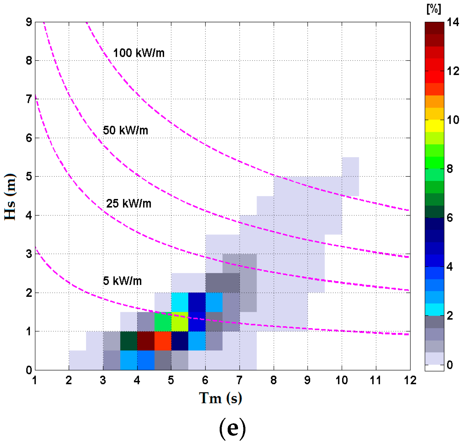
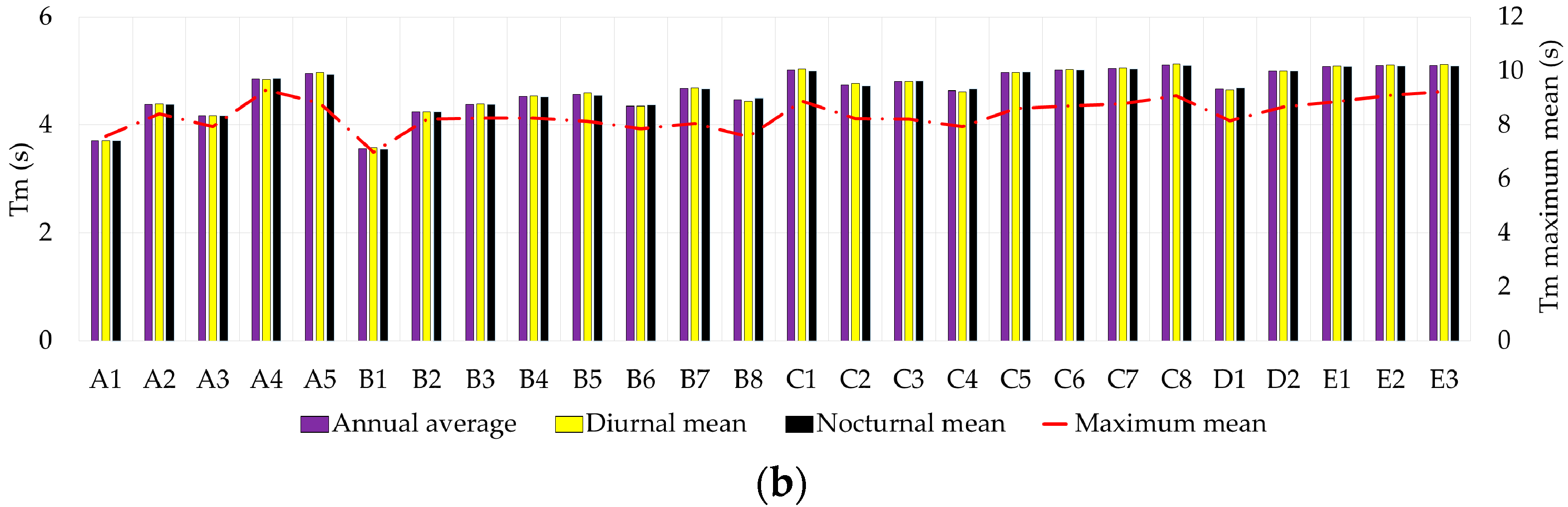
Figure 2 presents the wind conditions of the entire area studied corresponding to the 11-year period considered (2005–2015). Figure 2a illustrates the annual average, diurnal/nocturnal and maximum/mean values. In this study, the diurnal period is considered the interval from 6 to 18, while the nocturnal period from 18 to 6. ECMWF provided this data set. Following the analysis of the results, it can be noticed that the wind speed is rather constantly distributed in the Greek nearshore. By analyzing the wind conditions in the Ionian Sea, it can be mentioned that the wind tends to be more intense during the diurnal period, except for the reference point A5. The maximum mean value recorded in this region was 19.95 m/s (corresponding to the reference point A4 with an annual average of 6.13 m/s) while the minimum is 16.88 m/s (for the reference point A1). In addition, in the reference point A5, the energy potential has a quite balanced distribution, concerning the diurnal and nocturnal wind intensities. Regarding zone B (Aegean Sea), a rather different situation can be noticed. In this area, the points studied have a higher energy potential. The maximum value recorded was 22.05 m/s in the point B3, while the minimum corresponds to the point B8 (20.74 m/s). The annual average value recorded in the reference point B3 is 7.88 m/s. By analyzing the conditions in area B, it is noticed that the wind is more intense, globally speaking. Regarding now the diurnal and nocturnal distributions, it can also be noticed that the wind is more intense during the nocturnal period for 77.7% of the reference points considered. Zone C is the area associated with the Sea of Crete. By analyzing the data set, it cannot be identified a clear distribution between the diurnal and nocturnal wind intensities. Regarding the highest speed wind recorded in this area, this was 21.47 m/s in the reference point C2, characterized by an annual average value of 7.28 m/s. Areas D and E show a high energy potential. In the reference points considered for these two areas, the nocturnal period seems to be more energetic.
The maximum wind speed recorded in zone D is 20.67 m/s (point D2), while, in zone E, it is 20.62 m/s (point E1). As regards the annual average value, this is in the point D2 7.63 m/s and 7.66 m/s for the reference point E1.
Figure 2b illustrate the wind conditions at 80 m height for all of the 26 reference points according to the AVISO data set corresponding to the six-year interval (2010–2015).
By analyzing the results presented in Figure 2, it can be noticed that, in terms of the wind intensity, there is a considerable difference regarding the results corresponding to the two different data sets. Thus, by comparing Figure 2a,b, it can be mentioned that the AVISO data set had a more flattened distribution based on the annual average and the maximum mean values.
The different distributions illustrated in Figure 2 when considering the two data sets (ECMWF and AVISO) has as possible explanations the facts that ECMWF data is related to an 11-year time interval, while the AVISO data is only six years. At the same time, the resolutions in both space and time of the data are also quite different. Thus, for AVISO, the spatial resolution is 1° and the temporal resolution 24 h, while, for the ECMWF data, the spatial resolution is 0.75° and the temporal resolution 6 h.
The ECMWF data set was taken into account to continue the study due to the fact that this data set is more complex in terms of the parameters available and covers a longer time period. For example, ECMWF data contain information about wind, U and V components that are suitable in determining the wind direction. Moreover, the ECMWF data provides also a higher time resolution.
In choosing the most representative points for each of the five areas considered, the annual average values of the parameter U80 and also the maximum mean values were taken into account. Thus, by analyzing the ECMWF data set (Figure 2a), it can be noticed that, regarding the parameter U80, both the highest maximum mean and the annual average correspond to the reference points selected, which are A4 and A5 for zone A, B3 and B4 for zone B, C6 and C7 for zone C, D1 and D2 for zone D and E1 and E3 for zone E.
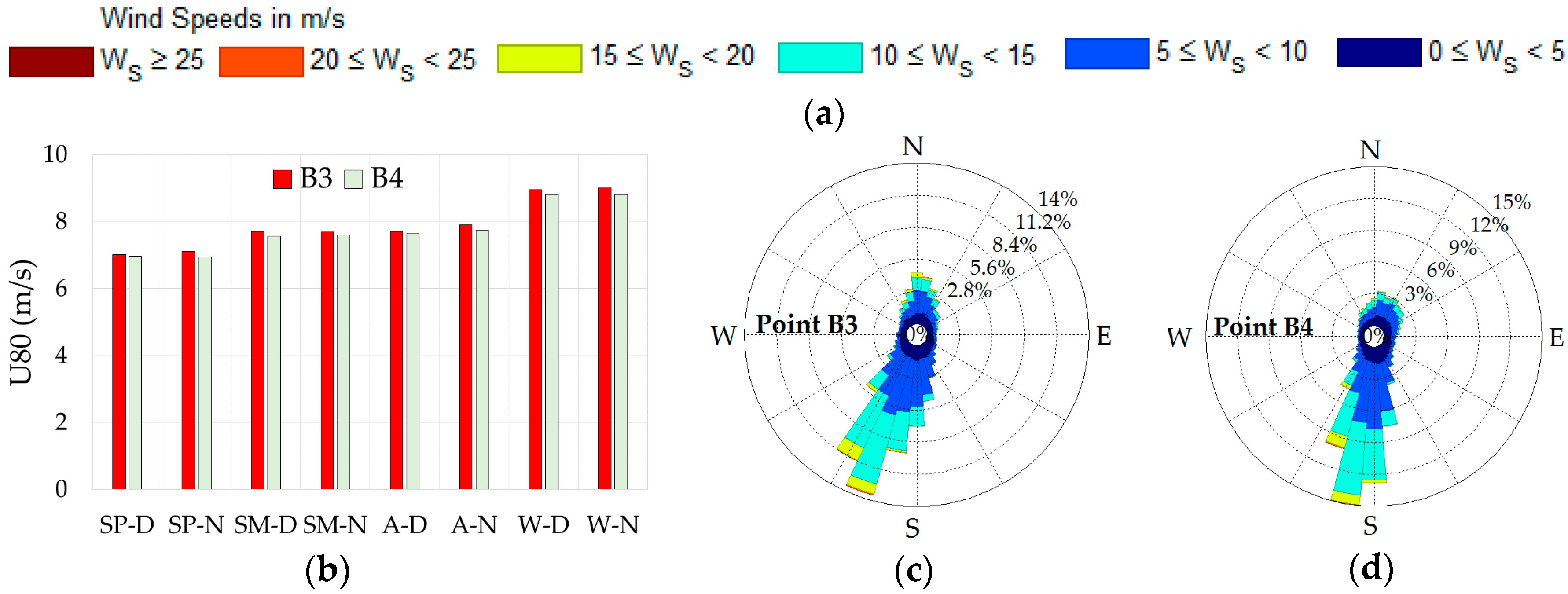
The time intervals considered are: spring diurnal (SP-D), spring nocturnal (SP-N), summer diurnal (SM-D), summer nocturnal (SM-N), autumn diurnal (A-D), autumn nocturnal (A-N), winter diurnal (W-D), and winter nocturnal (W-N).
Figure 3 illustrates the wind conditions at 80 m heights for the two points located in zone A. The distribution by classes indicates that the wind intensity is mainly less than 10 m/s. By analyzing the results corresponding to the reference point A4, it can be noticed that the wind blows mainly from the SE (Figure 3c), while, for the reference point A5 from the SW, E and ESE (Figure 3d). The distribution by intervals (seasons and day periods) is presented in Figure 3b. It can be observed that the wind is more intense during the winter period. During the wintertime, the mean values are in the range 7.34–7.75 m/s, while, for the other periods, in the range of 4.59–6.35 m/s. Regarding now the diurnal and nocturnal periods, it can be noticed that, for the point A4, the wind is more intense during the diurnal period, while, for the point A5, it tends to be more active during the nocturnal period.
For the zone B, the wind conditions are presented in Figure 4. It can be noticed that the wind energy potential during the diurnal and nocturnal periods is well balanced. The most energetic period for both points (B3 and B4) was winter diurnal (Figure 4b), while the less energetic one is spring nocturnal. The mean values for the winter period are in the range 8.81–9.01 m/s, while, for spring, summer and autumn, in the range 6.95–7.71 m/s. By analyzing Figure 4b, it can be also noticed that the wind intensity had an almost linear ascending trend. The wind conditions for the reference points B3 and B4 were similar (Figure 4b,c). The wind speed was mainly less than 15 m/s and its direction was from the SW.
Figure 5 shows the wind conditions at 80 m height corresponding to zone C. The distribution by classes indicates that the wind speed was mainly less than 15 m/s (Figure 5c,d). Figure 5c,d also show that, in the reference point C6, the main wind direction is from S-SE and SE while for point C7 from S and S-SE. According to the ECMWF data, in zone C, the wind was more intense during the winter period. The mean values are in the range 8.73–8.77 m/s, while for the other intervals in the range 6.31–7.44 m/s. By analyzing the diurnal and nocturnal wind distributions, it can be noticed that this varies for point C6. Regarding the reference point C7, the wind was slightly active during the nocturnal period. In addition, Figure 5b indicates that the reference point C6 stands out because it shows a high energy potential even during summer.
The ECMWF data shows that, for the reference point D1, the wind was more intense during the diurnal period (Figure 6b). Regarding the reference point D2, the wind was slightly active during the nocturnal period. Figure 6b also shows that the wind was more energetic during summer and winter. During the summer, the mean values were in the range 6.87–8.11 m/s, while during the winter, the mean wind speed values are in the range 7.40–8.29 m/s. Regarding spring and autumn, these were in the range 6.10–7.16 m/s. By analyzing the intensity, it can be noticed that, for both reference points, the wind speed was mainly less than 15 m/s (Figure 6c,d). Figure 6c,d also show that, in points D1 and D2, the wind direction is mainly from the SE.
Figure 7 illustrates the distribution of wind conditions for zone E in correspondence with the U80 parameter. The distribution (mean values) indicates that, in this region, the wind was more active during the winter. Thus, the wind speed mean values during winter were in the range 8.54–8.93 m/s, while during spring, summer and autumn in the range 7.03–7.96 m/s.
Figure 7c,d shows that the wind speeds are mainly less than 15 m/s. Regarding now zone E, the wind direction was mainly from S-SE in point E1 and S-SW and E-SE in point E3.
3.2. Analysis of Wave Intensity Distribution
Figure 7 shows a detailed picture of the wave conditions close to the Greek islands by evaluating the parameters Hs and Tm for all the 26 reference points. As defined in Equation (5), the wave power is a combination between the square of the significant wave height and the wave period. For this study, the ECMWF data set was taken into consideration due to the fact that this data set is more complex. The ECMWF data also contain information about the wave period and direction and also covers a longer time period. The most representative points in terms of the wave energy potential were selected having as a basis the mean values of the parameters Hs and Tm. Thus, 10 reference points have been selected for a detailed analysis, two for each of the five zones. By analyzing the ECMWF data set (Figure 8), it can be concluded that the most appropriate points for the analysis of the wave intensity distribution are the same as the reference points previously considered for the wind analysis (A4 and A5 for zone A, B3 and B4 for zone B, C6 and C7 for zone C, D1 and D2 for zone D and E1 and E3 for zone E). From this perspective, in this subsection, there will be evaluated the parameters significant wave height (Hs) and the wave period (Tm) in terms of their mean values for the diurnal and nocturnal intervals. In addition, the evolution of these parameters was studied with respect to the four seasons each divided into two intervals. Thus, the intervals studied are: spring diurnal (SP-D), spring nocturnal (SP-N), summer diurnal (SM-D), summer nocturnal (SM-N), autumn diurnal (A-D), autumn nocturnal (A-N), winter diurnal (W-D) and winter nocturnal (W-N).
The wave analysis, corresponding to the points A4 and A5, is presented in Figure 8. Regarding the parameter significant wave height, it can be noticed that it is an almost imperceptible difference of intensity between the diurnal and nocturnal intervals (Figure 9a,c). The analysis corresponding to each season can be seen in Figure 9b,d. By analyzing these figures, it can be concluded that, in the Ionian Sea basin in terms of significant wave height, the waves were more intense during the winter period and less intense during the summer.
Regarding the wave period, it can be noticed that the reference point A4 was characterized by lower values, on average by 14%.
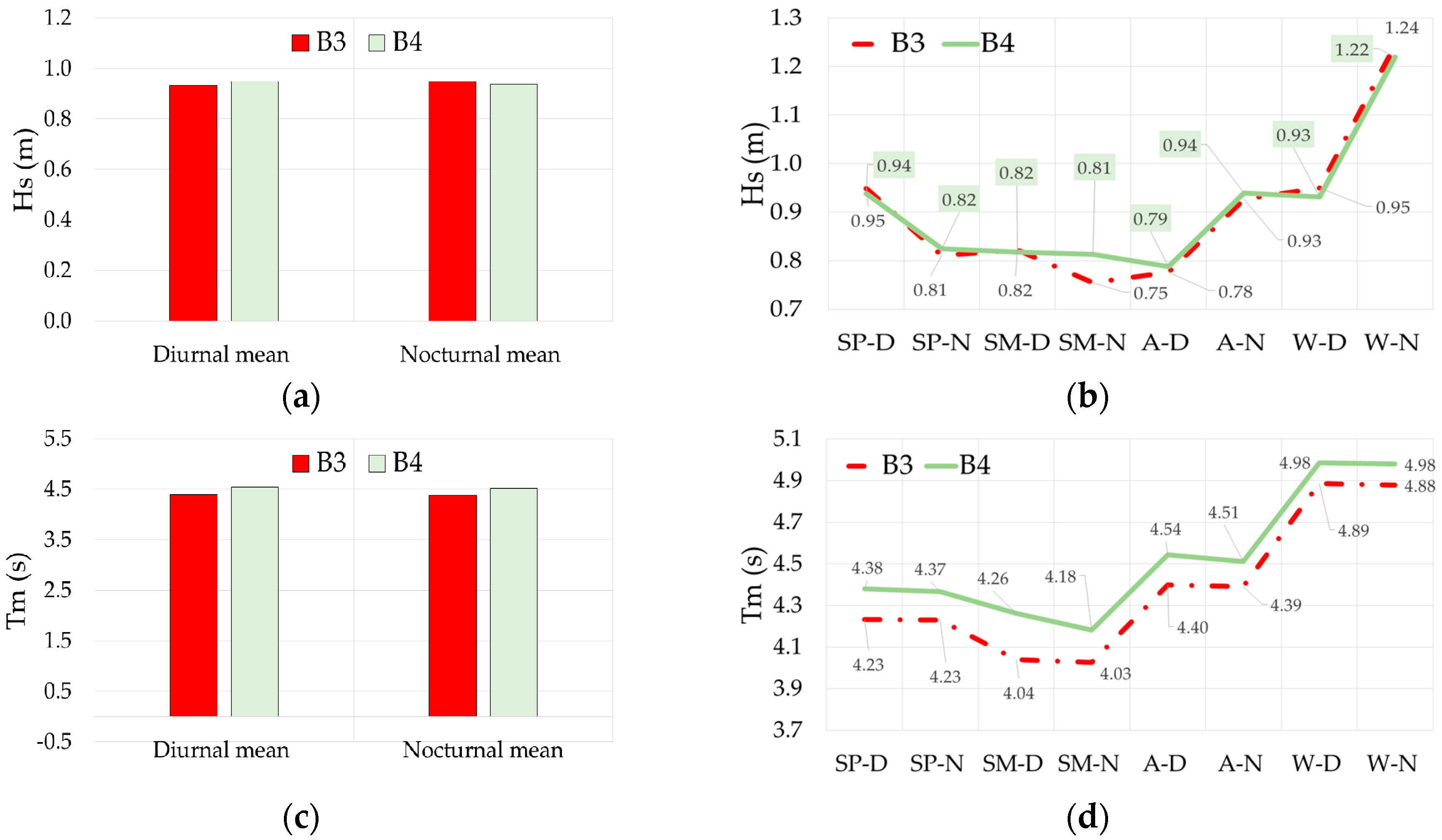
The histograms presented in Figure 10a,c present the evolution of the wave conditions in the points from the Aegean Sea. By analyzing the significant wave heights, diurnal against nocturnal, it can be noticed that there is practically no difference of intensity. The seasonal distribution shows that both points have rather similar characteristics in terms of significant wave height. The maximum mean value is equal to 1.24 m during winter nocturnal (point B3) while the minimum is 0.75 m during summer nocturnal (point B4) (Figure 10b). According to period, the waves in the point B4 have slightly higher periods (Figure 10c,d).
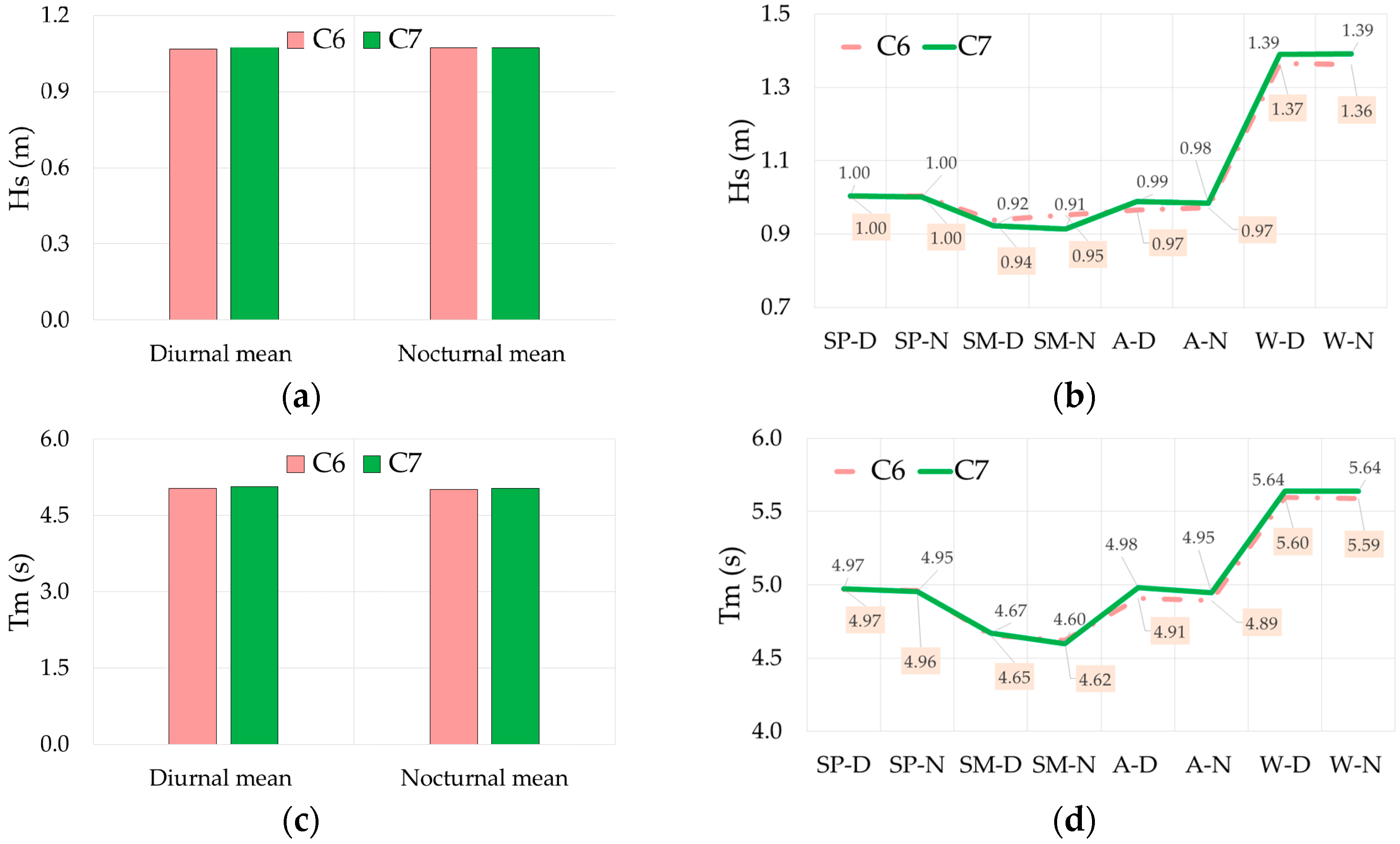
Figure 11 presents the analysis of the significant wave height and of the mean wave period for the points belonging to the Sea of Crete, corresponding to the time interval January 2005–December 2015. Regarding the parameter significant wave height, no noticeable differences can be observed by comparing the diurnal and nocturnal periods (Figure 11a). By analyzing the distribution by seasons, it can be noticed that both points had the same evolution. The highest values were recorded during winter diurnal nocturnal.
A detailed investigation of wave conditions for the zone D is presented in Figure 12. Thus, the histograms given in this figure show that point D2 has on average waves higher with 21.7% in terms of significant wave height and with 7.2% in terms of the mean wave period. As previously shown, winter is characterized by higher significant wave heights and periods (Figure 12c,d).
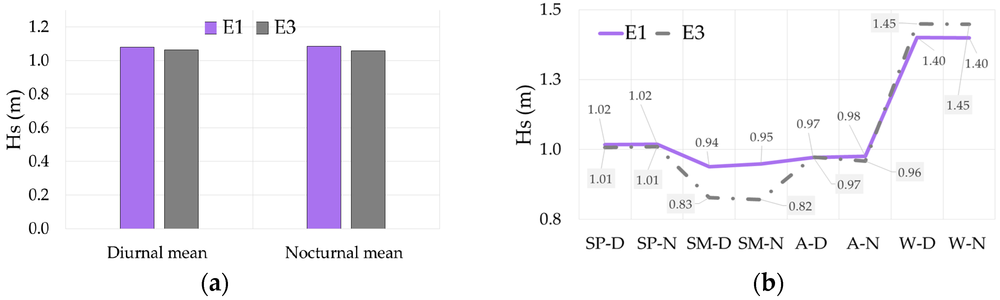
The significant wave height and mean period of the Libyan Sea points, corresponding to the time interval January 2005–December 2015 is presented in Figure 13. As it can be seen, the wave intensity is sensibly equal in both points. By analyzing Figure 13b,c, it can be noticed that, during the winter, the waves were higher by 50% compared to the summer. Regarding wave period, the same evolution is noticed in both locations. As in the previous cases, the highest values were recorded during the winter.
4. Discussion
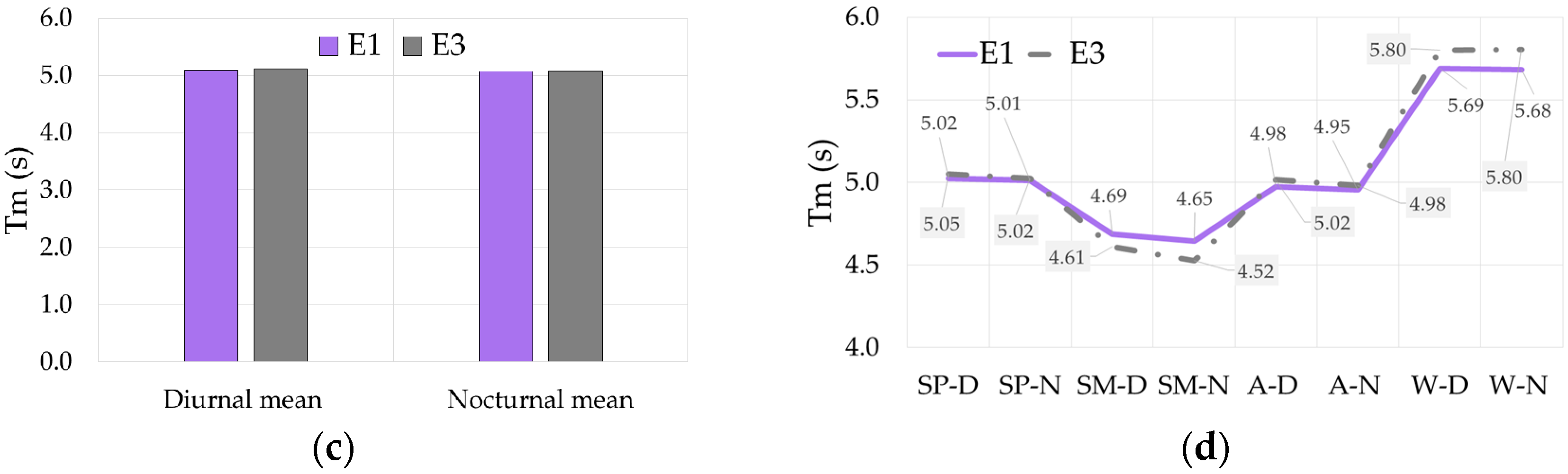
The wind power density (Pwind) is presented in Figure 14. By analyzing this parameter, it can be noticed that the points located in the proximity of Zakynthos island (A4) and Kythira Island (A5) have the lowest energy potential. Thus, the annual average value for the point A4 is 140.44 W/m2, while the maximum mean value is 4.84 kW/m2. Regarding the point A5, the annual average was 147.37 W/m2 and the maximum mean of 4.83 kW/m2. Another point with low energy potential is D1. Thus, the point D1 has the annual average of 198.25 W/m2 and a maximum mean of 4.73 KW/m2.
Three of the most energetic locations with respect to the wind power density were B3 (in the proximity of Cios Island, 2.41 km to shore), B4 (in the proximity of Tinos Island, 2.7 km to shore) and C6 (in the proximity of Crete, 2.27 km to shore). Regarding these points, the maximum value was in the range 6.03–6.57 kW/m2, while the annual average is in the range 286–298.96 W/m2.
In addition, for the remaining points, the annual average value is in the range 198.25–275.03 W/m2 while the maximum mean in the range 4.77–5.96 kW/m2.
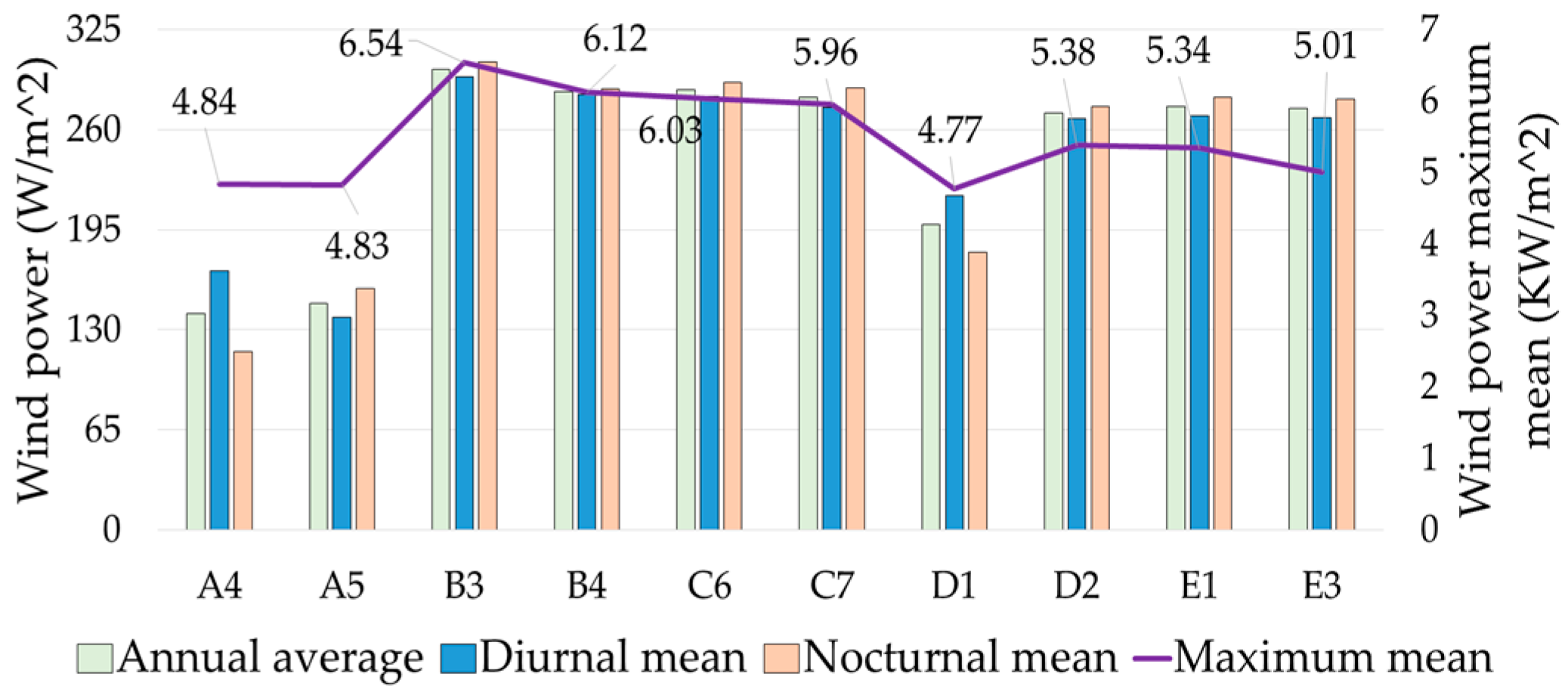
Further on, the Siemens SWT 3.6-120 wind turbine is considered to evaluate the wind potential. The wind turbine performance curve is represented in Figure 15 [40]. Considering the power variation with respect to the wind speed, a more detailed investigation of the wind conditions can be carried out. This includes parameters such as: operating capacity (OC%), rated capacity (RC%) and capacity factor (Cf%).
The capacity factor (Figure 16a) represents the ratio between the electric power produced by the turbine, Pwtgenerated, in a specific location and the maximum output, Prated, of a single Siemens SWT 3.6-120 system (6):
The operating time percentage of a wind turbine is indicated by the operating capacity parameter (Figure 16b). This parameter can be determined based on the cut-in wind speed (3 m/s) and the cut-out wind speed (25 m/s). The maximum performance of a wind turbine is highlighted by the rated capacity (Figure 15c). This parameter can be computed based on the rated speed (12.5 m/s) and the cut-out value.
By analyzing the reference points considered in the Ionian Sea, it can be noticed that this area is the least suitable for a wind turbine implementation. The capacity factor corresponding to these two points has a mean value of 32.6%. The operating capacity factor for these two points was high (A4 92.99% and A5 92.95%), while the rated capacity is rather small. This means that a turbine can operate with maximum efficiency for 8.34% of the time in the point A4 and 8.79% in A5.
According to this study, the best suitable areas for a wind turbine implementation are the areas corresponding to the Aegean Sea, Sea of Crete and Libyan Sea. Figure 16 illustrates that the zone B points have a total mean Cf value of 50.22% for B3 and 49.35% for B4. By analyzing the operating capacity, it was noticed that it is quite high, 94.32% for point B3 and 93.83% for B4. The rated capacity for this zone indicates that a wind turbine has to function on average 23.03% of the time for point B3 and 22.36% for B4. Regarding the seasonal distribution, it can be noticed that the RC parameter increases during the winter. The next best area for a wind turbine implementation is the Libyan Sea. The mean value of the capacity factor of both zone E points is 47.64%. Regarding the operating capacity, it can be noticed that this has the values 96.98% in point E1 and 98.26% in E2. By analyzing the rated capacity, zone E has a mean of 16.49%. The Sea of Crete energy potential in the points studied is rather similar to that from area E. The point C6 is characterized by a Cf value of 49%, OC of 96.88 and RC of 17.51%, while point C7 by a Cf of 48.33%, OC of 96.99 and RC of 17.43%.
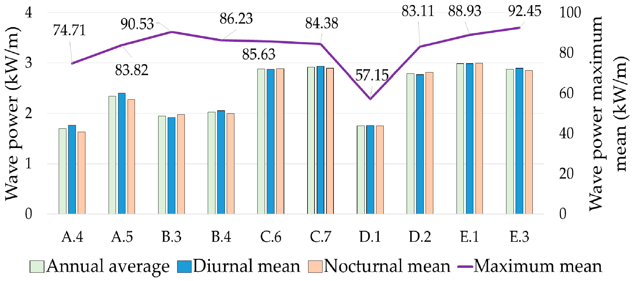
The wave power represents the energy flux in kilowatts per meter of the wave crest (kW/m). The wave power corresponding to the 11-year interval, from January 2005 to December 2015, structured on annual average, diurnal mean, nocturnal mean and maximum mean, is presented in Figure 17.
The wave power distribution presented in Figure 17 for the 10 reference points shows the differences between the zones studied. By analyzing the wave power density, it can be noticed that the points C6, C7 and E1 have the highest energy potential in terms of the wave power. For these points, the annual average wave power is in the range 2.88–2.99 kW/m. In addition, the points A4 and D1 have the lowest energy potential. The annual average value for the point A4 is 1.7 kW/m, while for the point D1 is 1.76 kW/m. The Aegean Sea points, B3 and B4, also recorded a low energy potential. The wave power values are in the range 1.95 kW/m to 2.02 kW/m.
The maximum mean value recorded for the 11-year interval in the point E3 is 92.45 kW/m.
Looking now at Figure 14 and Figure 17 altogether, some similarities and differences in terms of the wind and wave energy in some locations can be noticed. The most significant difference is that, while the maximum values of the wind power correspond to the locations from the Aegean Sea, in terms of wave power, the highest potential occurs in the Sea of Crete. Actually, in this area, the wind power can also be considered relevant. Thus, according to the data presented in the two figures, in terms of wave power, the coastal environment of Crete is 45.73% higher than in the Aegean Sea, while, in terms of wind power, it is only 2.91% smaller. At this point, the specific patterns of wave generation and propagation in the areas targeted should also be considered, which are extensively discussed in Makris et al. [24]. From this perspective, in the area of the Greek islands, the strongest waves are not always correlated with the highest wind conditions.
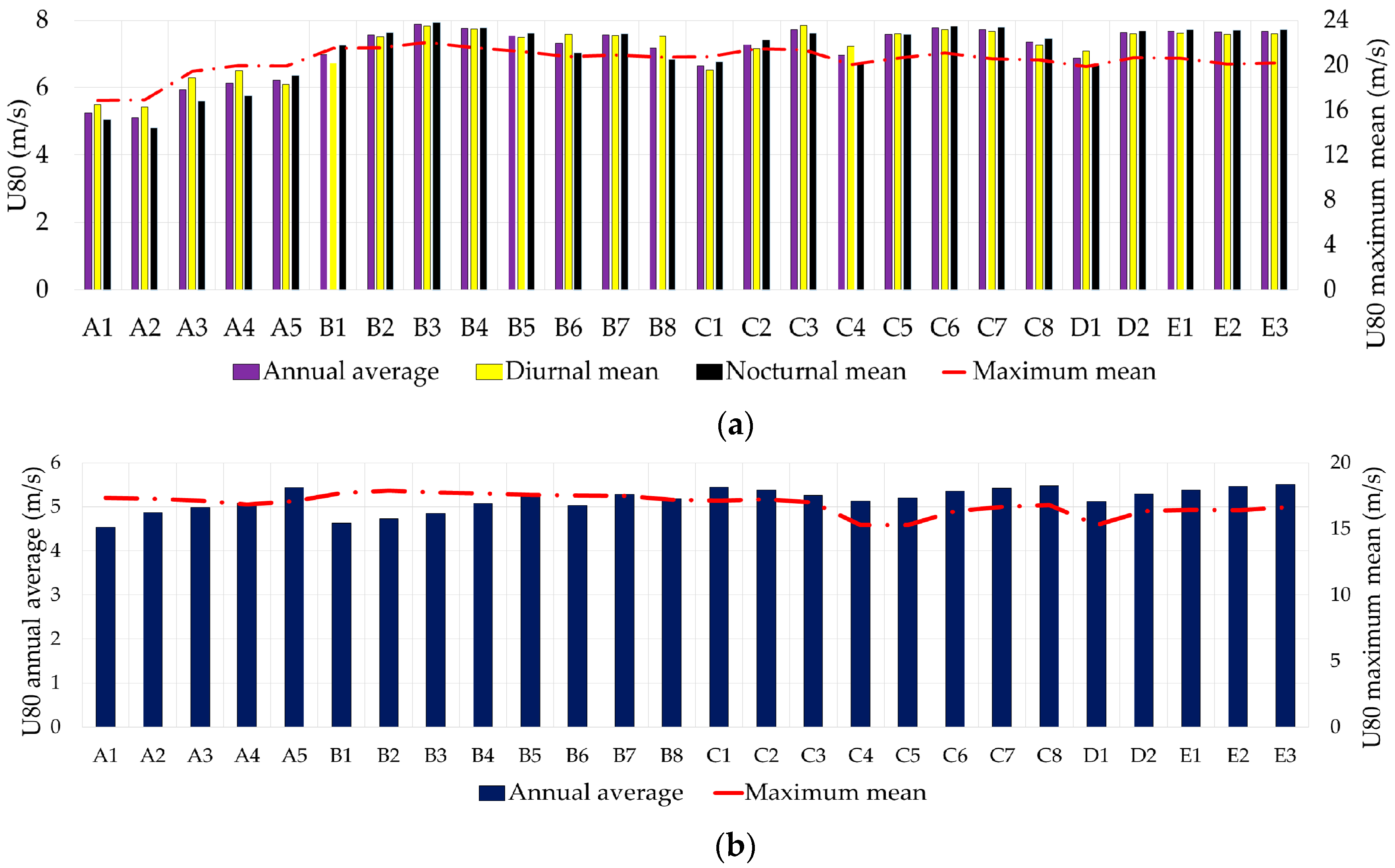
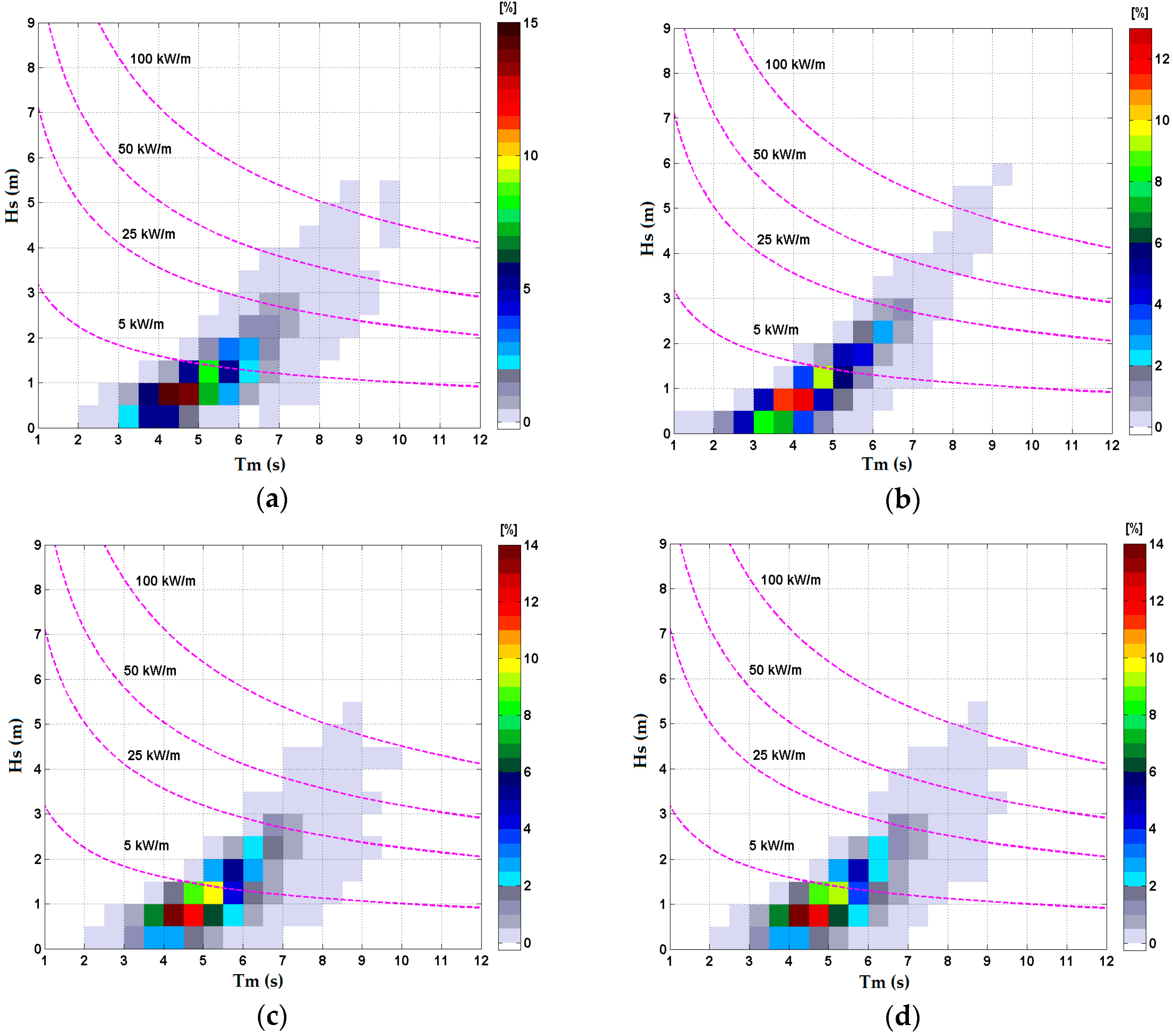
The bivariate distributions for the wave parameters (Hs and Tm) corresponding to five reference points are illustrated in Figure 18. These diagrams present the distribution of the sea states for each zone, being defined by the parameters significant wave height (Hs) and mean wave period (Tm), and they were designed for the 11-year interval from 1 January 2005 to 31 December 2015. Furthermore, the wave power isolines are represented for four different energy levels (5 kW/m, 25 kW/m, 50 kW/m, 100 kW/m).
Figure 18a corresponds to the point A5 and shows that the bulk of occurrences is located around the isoline of 5 kW/m. Figure 18b corresponds to the B3 point, and it can be noticed that, although most of the occurrences are also close to the isoline of 5 kW/m, the energy is more focused than in all other cases. Moreover, relevant occurrences can also be noticed near the isoline of 25 kW/m.
Regarding now the points C6, D2 and E3, it can be noticed that the energy is more widely spread and the bulk of occurrences are found closer to the isoline of 25 kW/m.
5. Conclusions
In the present work, both data sources considered cover the entire marine environment of the Greek coastal environment. The difference between the two data sets consists mainly in the fact that the first one having a higher temporal and spatial resolution, while the second can provide information without the restriction of the geographical characteristics. On the other hand, ECMWF provides information about wind, including the U and V components, that are suitable in determining the wind direction and also information about wave period and direction. Furthermore, ECMWF also covers a longer time period.
Analyzing the wind and wave dynamics in the target areas, it can be concluded that the nearshore and offshore areas close to the Greek islands have a significant energy potential.
By analyzing the Greek National Renewable Energy Action Plan, developed in the scope of the directive 2009/28/EC, the Greek Ministry of Environment, Energy & Climate Change estimates a balancing between the conventional and RES exploitation methods. Thus, until 2020, an RES energy production of 41.7% from the total installed capacity (68 TWh) is desired. Given this context, it can be concluded that the wind and wave conditions in the coastal areas studied may represent a suitable alternative for reducing the gap between RES and the conventional methods. The synergy between the RES studied (wind and waves) can thus induce a sustainable development in the Greek economy.
At this point, it has to be highlighted that Greece geographical positioning and characteristics, being a peninsular and insular country with a 17,400 km of coast length and a maritime surface of 114,507 km2, has an important potential in RES exploitation.
The objective of this work is to present a more comprehensive picture of the wind and wave energy potential close to the Greek islands due to the fact that in this area the synergy between these two RES has not been extensively evaluated in the past. In this study, two different datasets have been analyzed. The first covers the 11-year time interval between 1 January 2005 to 31 December 2015 and was provided by ECMWF, while the second one is provided by AVISO and covers the six-year interval 1 January 2010 to 31 December 2015.
The targeted area of the study is located in the Mediterranean Sea. More precisely, there were analyzed locations found in the perimeter of the Ionian (A), Aegean (B), Crete (C), Levantine (D) and Libyan (E) seas. When initially analyzed, 26 reference points were considered. For a more detailed investigation, the analysis was further focused on the 10 most representative points in terms of energy potential. Thus, for each of the five areas considered, two locations were selected. The aim of the study was to identify the most energetic locations, from the perspective of future wind turbines and WEC implementation. Thus, parameters such as U80, Hs and Tm were assessed. By processing and analyzing the dynamics of these parameters, it was possible to determine the energy potential of the Greek islands as well as the synergy between the two resources.
Regarding the wind energy potential, it can be noticed that a higher potential is in the proximity of Cios and Tinos islands (Aegean Sea), Crete and Dia islands (Sea of Crete), Kasos Island (Levantine Sea) and south of Crete (Libyan Sea). In these areas, the U80 mean annual values are in the range 7.63–7.88 m/s, while the annual average wind power is in the range 270.94–298.96 W/m2.
By analyzing the wave power density, it can be observed that the points C6, C7 and E1 have the highest energy potential. For these points, the annual average wave power was in the range 2.9–3 kW/m.
Furthermore, a Siemens SWT 3.6-120-wind turbine power variation in respect to the wind speed was considered to evaluate the energy potential. A detailed investigation was conducted. This includes the analysis of the following parameters: operating capacity (OC%), rated capacity (RC%) and capacity factor (Cf%). The resulted data indicate the fact that the capacity factor is in the range of 32.02–50.23%, the minimum mean value being recorded south of Zakynthos Island, while the maximum was recorded west of Cios Island. The maximum performance of a wind turbine is highlighted by the rated capacity parameter (RC%). The results indicate that this parameter is in the range 8.32% (south of Zakynthos Island) to 23.03% (west of Cios Island). The operating time percentage of a wind turbine is indicated by the operating capacity parameter (OC %). By analyzing the data, it can be noticed that a Siemens SWT 3.6-120 wind turbine had a mean operating capacity of 95.31%.
The bivariate distributions of the wave parameters, north and south of Crete and south of Kasos Island, illustrate that the energy potential is more spread and the bulk of occurrences are found closer to the 25 kW/m isoline. Regarding the areas west of Kythira and Cios islands, the bulk of occurrences are located around the isoline of 5 kW/m.
Future works will be focused on the identification of the most relevant hot spots in the Greek island environment by performing high resolution simulations with phase averaged spectral wave models. Subsequently, another issue is related to evaluations of the performances of various devices for wind and wave energy conversion in the hot spots identified above.
Finally, it can be concluded that the Greek marine environment has relevant wind energy resources as well as a good potential for hybrid wind-waves energy exploitation, especially from the perspective of the development of the WEC devices especially designed for the small amplitude waves.
Acknowledgments
This work was carried out in the framework of the project proposal REMARC, submitted under the number PN-III-P4-IDPCE-2016-0017 to the Romanian Executive Agency for Higher Education, Research, Development and Innovation Funding, UEFISCDI. The authors would like also to express their gratitude to the reviewers for their constructive suggestions and observations that helped in improving the present work.
Author Contributions
Daniel Ganea and Valentin Amortila has gathered, processed and analyzed the data. Elena Mereuta has done the literature review and drawn the main conclusions. Eugen Rusu has guided this research and discussed the data. All of the authors have participated in the writing of the paper. The final manuscript has been approved by all authors.
Conflicts of Interest
The authors declare no conflict of interest.
Nomenclature
| AVISO | archiving, validation and interpretation of satellite oceanographic |
| Cf | capacity factor |
| DER | distributed energy resources |
| ECMWF | European Centre for Medium-Range Weather Forecasts |
| Hs | wave height |
| LCOE | levelized the cost of electricity |
| MG | microgrid |
| MWP | mean wave period |
| OC | operating capacity |
| Pwave | wave power density index |
| Pwtgenerated | the output energy generated by a wind turbine |
| Pwind | wind power density index |
| RC | rated capacity |
| RES | renewable energy resources |
| SWH | significant height of combined wind-waves and swell |
| Tm | wave periodicity |
| U10 | wind speed at 10 m |
| U80 | wind speed at 80 m |
| WEC | wave energy convertor |
References
- Ansell, A.D.; Gibson, R.N.; Barnes, M. An Annual Review Oceanography and Marine Biology; Taylor & Francis: Abingdon, UK, 2005; Volume 35. [Google Scholar]
- Marineplan. Available online: http://www.marineplan.es/ES/fichas_kml/iho.html (accessed on 11 December 2016).
- Worldatlas. Available online: http://www.worldatlas.com/aatlas/infopage/seaofcrete.htm (accessed on 11 December 2016).
- Revolvy. Available online: https://www.revolvy.com/main/index.php?s=Levantine%20Sea (accessed on 11 December 2016).
- Hellenic National Meteorological Service. Available online: www.hnms.gr/hnms/english/meteorology/full_story_html?dr_url=%2Fhnms%2Fdocrep%2Fdocs%2Fmisc%2FClimateOfGreek (accessed on 5 December 2016).
- YPEKA. Available online: http://www.ypeka.gr/LinkClick.aspx?fileticket=CEYdUkQ719k%3D (accessed on 8 December 2016).
- Marzband, M.; Ardeshiri, R.R.; Moafi, M.; Uppal, H. Distributed generation for economic benefit maximization through coalition formation based on Game Theory. Int. Trans. Electr. Energy Syst. 2017, 27, e2313. [Google Scholar] [CrossRef]
- Marzband, M.; Parhizi, N.; Adabi, J. Optimal energy management for stand-alone microgrids based on multi-period imperialist competition algorithm considering uncertainties: Experimental validation. Int. Trans. Electr. Energy Syst. 2015, 26, 1358–1372. [Google Scholar] [CrossRef]
- Marzband, M.; Ghazimirsaeid, S.S.; Uppal, H.; Fernando, T. A real-time evaluation of energy management systems for smart hybrid home Microgrids. Electr. Power Syst. Res. 2016, 143, 624–633. [Google Scholar] [CrossRef]
- Marzband, M.; Moghaddamb, M.M.; Akoredec, M.F.; Khomeyranib, G. Adaptive load shedding scheme for frequency stability enhancement in microgrids. Electr. Power Syst. Res. 2016, 140, 78–86. [Google Scholar] [CrossRef]
- Marzband, M.; Javadi, M.; Domínguez-García, J.L.; Moghaddam, M.M. Non-cooperative game theory based energy management systems for energy district in the retail market considering DER uncertainties. IET Gener. Transm. Distrib. 2016, 10, 2999–3009. [Google Scholar] [CrossRef]
- Marzband, M.; Parhizi, N.; Savaghebi, M.; Guerrero, J.M. Distributed smart decision-making for a multi-microgrid system based on a hierarchical interactive architecture. IEEE Trans. Energy Convers. 2016, 31, 637–648. [Google Scholar] [CrossRef]
- Marzband, M.; Azarinejadian, F.; Savaghebi, M.; Guerrero, J.M. An optimal energy management system for islanded microgrids based on multiperiod artificial bee colony combined with markov chain. IEEE Syst. J. 2015, 100, 1–11. [Google Scholar] [CrossRef]
- Rusu, L.; Onea, F. Assessment of the performances of various wave energy converters along the European continental coasts. Energy 2015, 82, 889–904. [Google Scholar] [CrossRef]
- Rusu, E. Evaluation of the wave energy conversion efficiency in various coastal environments. Energies 2014, 7, 4002–4018. [Google Scholar] [CrossRef]
- Rusu, E.; Onea, F. Estimation of the wave energy conversion efficiency in the Atlantic Ocean close to the European islands. Renew. Energy 2016, 85, 687–703. [Google Scholar] [CrossRef]
- Silva, D.; Rusu, E.; Soares, C.G. Evaluation of various technologies for wave energy conversion in the portuguese nearshore. Energies 2013, 6, 1344–1364. [Google Scholar] [CrossRef]
- Morim, J.; Cartwright, N.; Etemad, S.A.; Strauss, D.; Hemer, M. A review of wave energy estimates for nearshore shelf waters off Australia. Int J. Mar. Energy 2014, 7, 57–70. [Google Scholar] [CrossRef]
- Quirapas, M.A.J.R.; Lin, H.; Abundo, M.L.S.; Brahim, S.; Santos, D. Ocean renewable energy in Southeast Asia: A review. Renew. Sustain. Energy Rev. 2015, 41, 799–817. [Google Scholar] [CrossRef]
- Rusu, L.; Onea, F. The performance of some state-of-the-art wave energy converters in locations with the worldwide highest wave power. Renew. Sustain. Energy Rev. 2017, 75, 1348–1362. [Google Scholar] [CrossRef]
- Rusu, E.; Onea, F. Study on the influence of the distance to shore for a wave energy farm operating in the central part of the Portuguese nearshore. Energy Convers. Manag. 2016, 114, 209–223. [Google Scholar] [CrossRef]
- Uihlein, A.; Magagna, D. Wave and tidal current energy—A review of the current state of research beyond technology. Renew. Sustain. Energy Rev. 2016, 58, 1070–1081. [Google Scholar] [CrossRef]
- Zanuttigh, B.; Angelelli, E.; Bellotti, G.; Romano, A.; Krontira, Y.; Troianos, D.; Suffredini, R.; Franceschi, G.; Cantù, M.; Airoldi, L.; et al. Boosting Blue Growth in a Mild Sea: Analysis of the Synergies Produced by a Multi-Purpose Offshore Installation in the Northern Adriatic, Italy. Sustainability 2015, 7, 6804–6853. [Google Scholar] [CrossRef]
- Makris, C.; Galiatsatou, P.; Tolika, K.; Anagnostopoulou, C.; Kombiadou, K.; Prinos, P.; Velikou, K.; Kapelonis, Z.; Tragou, E.; Androulidakis, Y.; et al. Climate change effects on the marine characteristics of the Aegean and Ionian Seas. Ocean Dyn. 2016, 66, 1603–1635. [Google Scholar] [CrossRef]
- Onea, F.; Deleanu, L.; Rusu, L.; Georgescu, C. Evaluation of the wind energy potential along the Mediterranean Sea coasts. Energy Explor. Exploit. 2016, 34, 766–792. [Google Scholar] [CrossRef]
- Onea, F.; Raileanu, A.; Rusu, E. Evaluation of the Wind Energy Potential in the Coastal Environment of Two Enclosed Seas. Adv. Meteorol. 2015, 2015, 808617. [Google Scholar] [CrossRef]
- Petrakopoulou, F. The Social Perspective on the Renewable Energy Autonomy of Geographically Isolated Communities: Evidence from a Mediterranean Island. Sustainability 2017, 9, 327. [Google Scholar] [CrossRef]
- Kim, G.; Lee, M.E.; Lee, K.S.; Park, J.S.; Jeong, W.M.; Kang, S.K.; Soh, J.G.; Kim, H. An overview of ocean renewable energy resources in Korea. Renew. Sustain. Energy Rev. 2012, 16, 2278–2288. [Google Scholar] [CrossRef]
- Zanuttigh, B.; Angelelli, E.; Kortenhaus, A.; Koca, K.; Krontira, Y.; Koundouri, P. A methodology for multi-criteria design of multi-use offshore platforms for marine renewable energy harvesting. Renew. Energy 2016, 85, 1271–1289. [Google Scholar] [CrossRef]
- Zabihian, F.; Fung, A.S. Review of marine renewable energies: case study of Iran. Renew. Sustain. Energy Rev. 2011, 15, 2461–2474. [Google Scholar] [CrossRef]
- Wang, S.J.; Yuan, P.; Li, D.; Jiao, Y.H. An overview of ocean renewable energy in China. Renew. Sustain. Energy Rev. 2011, 15, 91–111. [Google Scholar] [CrossRef]
- Hutcheson, F.; Andrés, A.; Jeffrey, H. Risk vs. Reward: A Methodology to Assess Investment in Marine Energy. Sustainability 2016, 8, 873. [Google Scholar] [CrossRef]
- Jinchao, L.; Xian, G.; Jinying, L. A Comparison of Electricity Generation System Sustainability among G20 Countries. Sustainability 2016, 8, 1276. [Google Scholar] [CrossRef]
- Onea, F.; Rusu, E. The expected efficiency and coastal impact of a hybrid energy farm operating in the Portuguese nearshore. Energy 2016, 97, 411–423. [Google Scholar] [CrossRef]
- Perez-Collazo, C.; Greaves, D.; Iglesias, G. A review of combined wave and offshore wind energy. Renew. Sustain. Energy Rev. 2015, 42, 141–153. [Google Scholar] [CrossRef]
- Zanopol, A.T.; Onea, F.; Rusu, E. Coastal impact assessment of a generic wave farm operating in the Romanian nearshore. Energy 2014, 72, 652–670. [Google Scholar] [CrossRef]
- Zanopol, A.T.; Onea, F.; Rusu, E. Evaluation of the coastal influence of a generic wave farm operating in the Romanian nearshore. J. Environ. Prot. Ecol. 2014, 15, 597–605. [Google Scholar]
- Mendoza, E.; Silva, R.; Zanuttigh, B.; Angelelli, E.; Andersen, T.L.; Martinelli, L.; Nørgaard, J.Q.H.; Ruol, P. Beach response to wave energy converter farms acting as coastal defence. Coast. Eng. 2014, 87, 97–111. [Google Scholar] [CrossRef]
- Kubik, M.L; Coker, P.J; Hunt, C. Using meteorological wind data to estimate turbine generation output: A sensitivity analysis. In Proceedings of the World Renewable Energy Congress—Sweden, Linköping, Sweden, 8–13 May 2011; pp. 4074–4081. [Google Scholar]
- Thoroughly Tested, Utterly Reliable Siemens Wind Turbine SWT-3.6-120. Available online: http://www.energy.siemens.com/ru/pool/hq/power-generation/wind-power/E50001-W310-A169-X-4A00_WS_SWT_3-6_120_US.pdf (accessed on 5 December 2016).
Figure 1.
The geographical positions of the 26 reference points: (A) Ionian Sea; (B) Aegean Sea; (C) Sea of Crete; (D) Levantine Sea; and (E) Libyan Sea (figure processed from Google Earth (2017)).
Figure 1.
The geographical positions of the 26 reference points: (A) Ionian Sea; (B) Aegean Sea; (C) Sea of Crete; (D) Levantine Sea; and (E) Libyan Sea (figure processed from Google Earth (2017)).
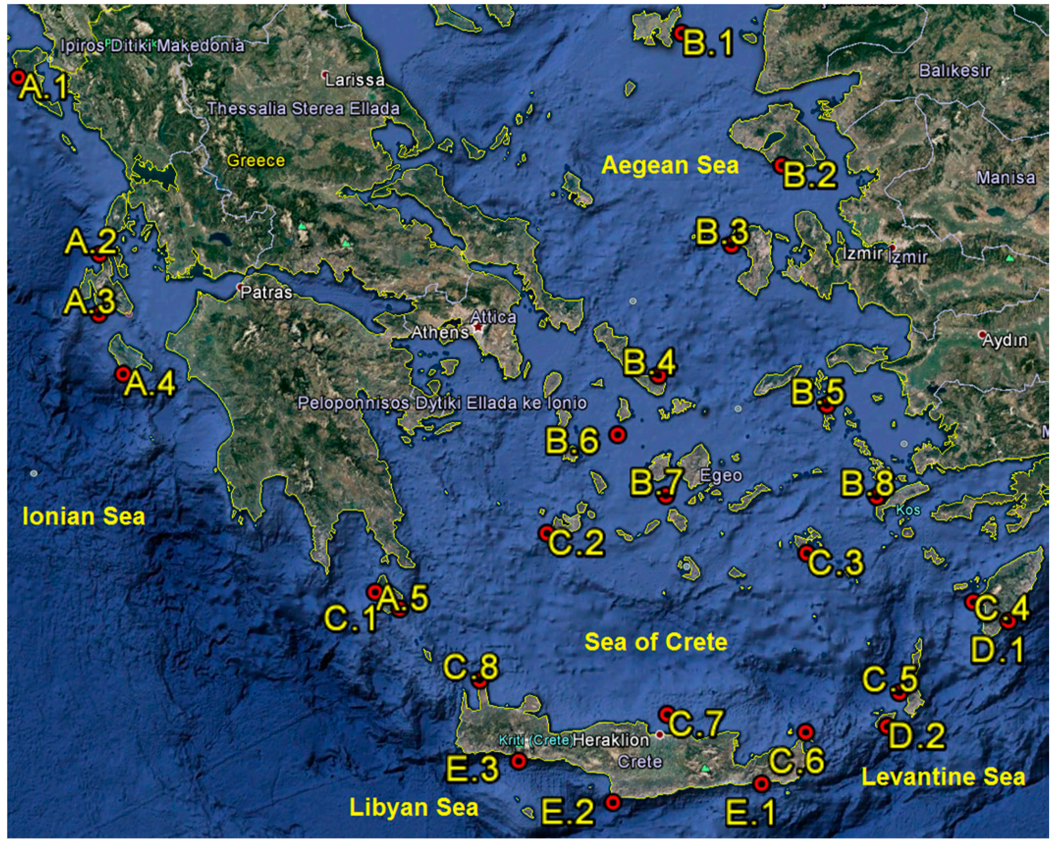
Figure 2.
Wind speed at 80 m height, evaluation corresponding to all 26-reference points. ECMWF data were processed (a) for the 11-year period (2005–2015), and AVISO data set (b) for the 6-year period (2010–2015).
Figure 2.
Wind speed at 80 m height, evaluation corresponding to all 26-reference points. ECMWF data were processed (a) for the 11-year period (2005–2015), and AVISO data set (b) for the 6-year period (2010–2015).

Figure 3.
Zone A wind speed evaluation at 80 m height; (a) wind speed intervals associated with the wind rose charts; (b) wind speed mean values for different intervals of the period studied (1 January 2005 to 31 December 2015.); (c) wind roses corresponding to point A4; (d) wind roses corresponding to point A5.
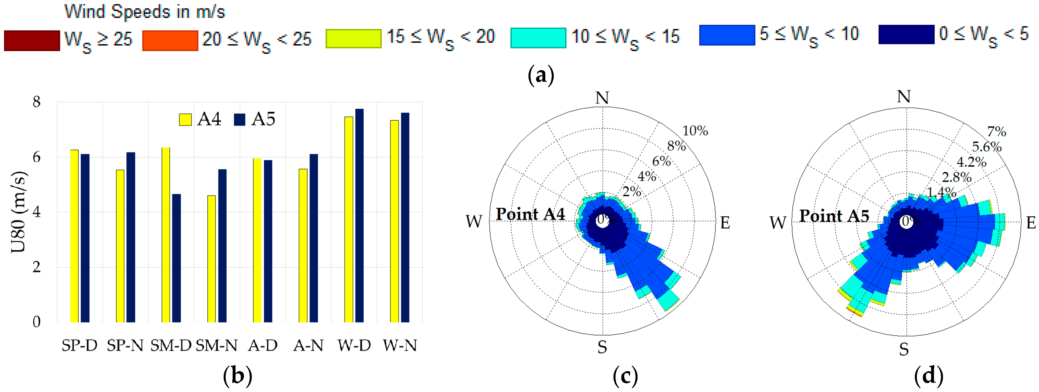
Figure 4.
Zone B wind speed evaluation at 80 m height; (a) wind speed intervals associated with the wind rose charts; (b) wind speed mean values for different intervals of the period studied (1 January 2005 to 31 December 2015.); (c) wind roses corresponding to point B3; (d) wind roses corresponding to point B4.

Figure 5.
Zone C wind speed evaluation at 80 m height; (a) wind speed intervals associated with the wind rose charts; (b) wind speed mean values for different intervals of the period studied (1 January 2005 to 31 December 2015.); (c) wind roses corresponding to point C6; (d) wind roses corresponding to point C7.
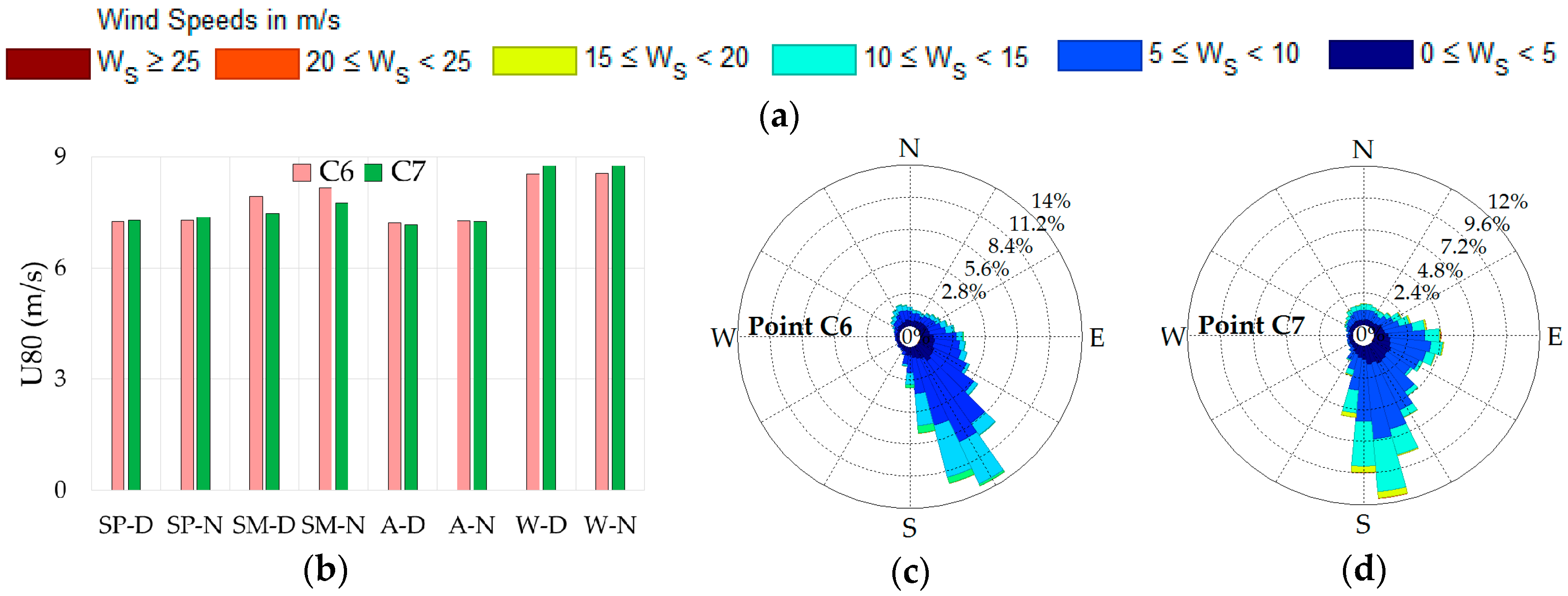
Figure 6.
Zone D wind speed evaluation at 80 m height; (a) wind speed intervals associated with the wind rose charts; (b) wind speed mean values for different intervals of the period studied (1 January 2005 to 31 December 2015.); (c) wind roses corresponding to point D1; (d) point D2.
Figure 6.
Zone D wind speed evaluation at 80 m height; (a) wind speed intervals associated with the wind rose charts; (b) wind speed mean values for different intervals of the period studied (1 January 2005 to 31 December 2015.); (c) wind roses corresponding to point D1; (d) point D2.
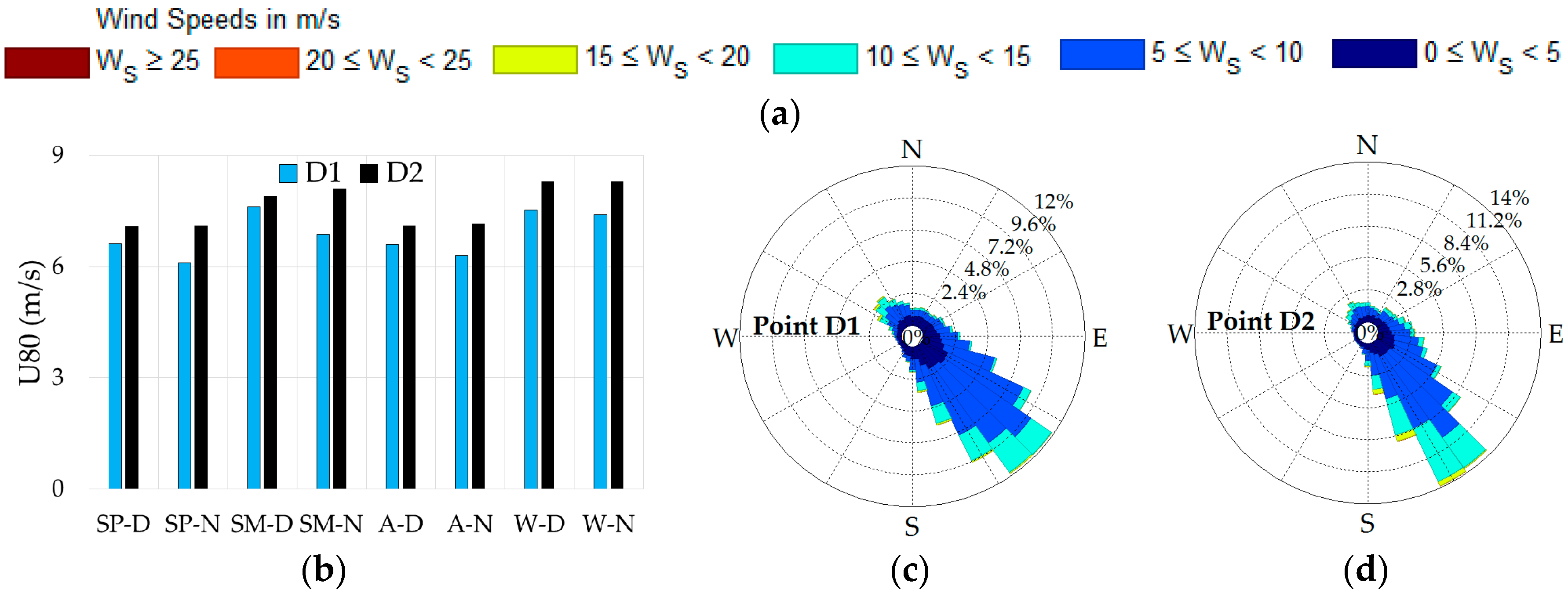
Figure 7.
Zone E wind speed evaluation at 80 m height; (a) wind speed intervals associated with the wind rose charts; (b) wind speed mean values for different intervals of the period studied (1 January 2005 to 31 December 2015.); (c) wind roses corresponding to point E1; (d) wind roses corresponding to point E3.
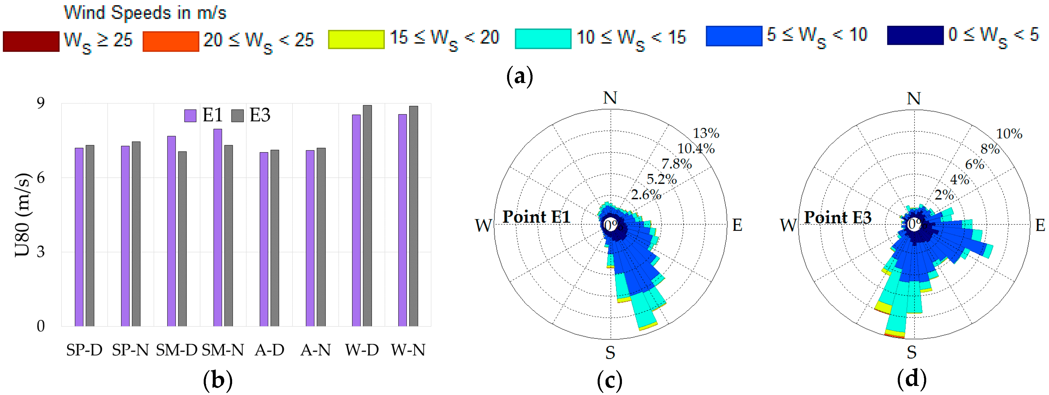
Figure 8.
Main wave parameters, evaluation corresponding to all 26-reference points. ECMWF data were processed (a) significant wave height (m); (b) wave period.
Figure 8.
Main wave parameters, evaluation corresponding to all 26-reference points. ECMWF data were processed (a) significant wave height (m); (b) wave period.
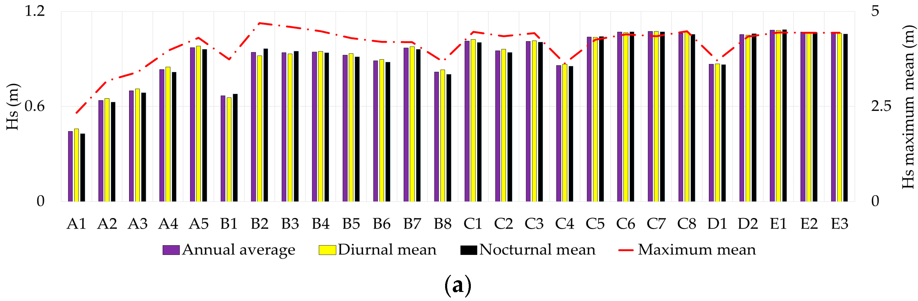

Figure 9.
Zone A, evaluation of the wave conditions considering the ECMWF data for the 11-year interval 2005–2015; (a) Hs mean values comparison of diurnal against nocturnal for total time; (b) Hs mean values comparison of diurnal against nocturnal for each season; (c) Tm mean values comparison of diurnal against nocturnal for total time; (d) Tm mean values comparison of diurnal against nocturnal for each season.
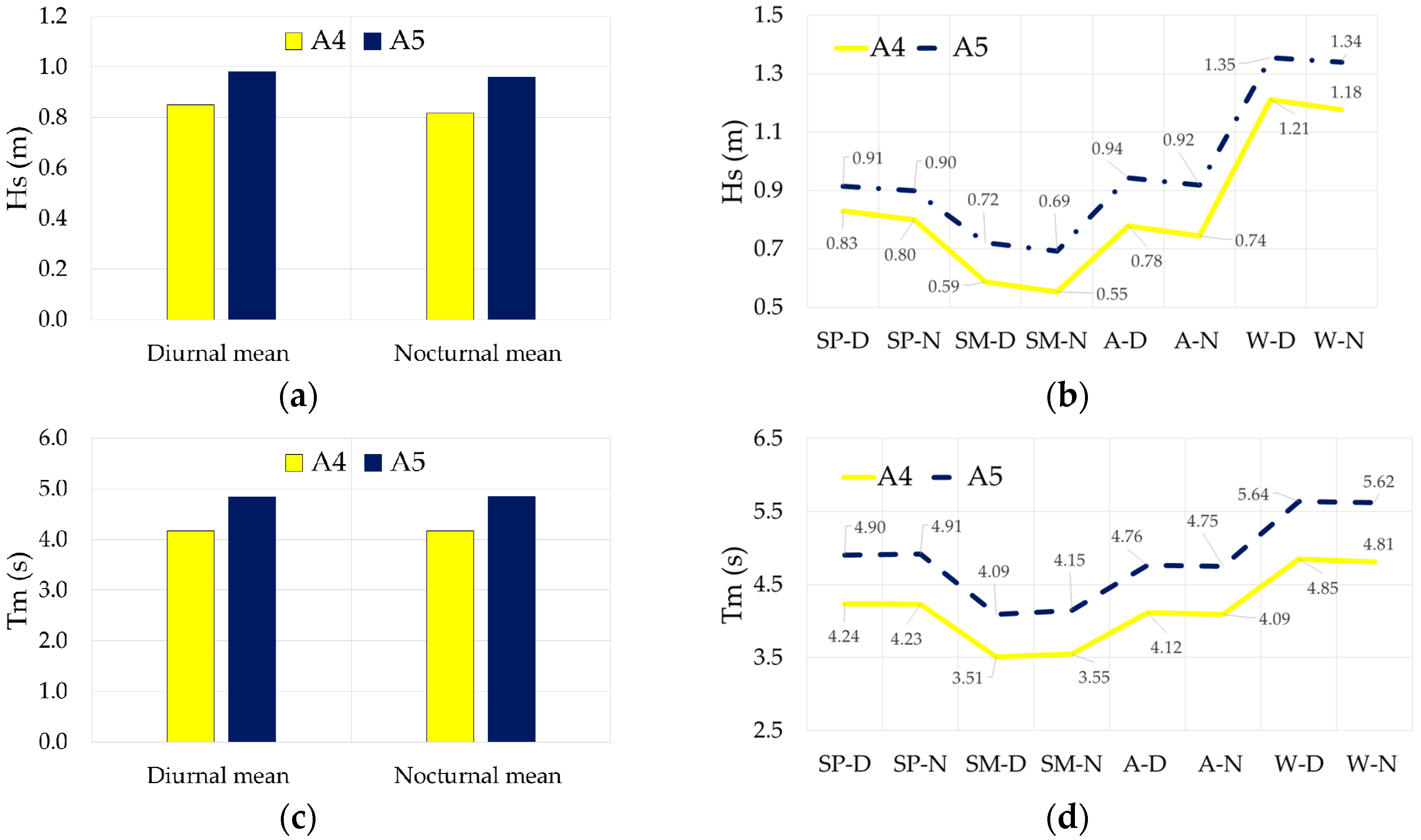
Figure 10.
Zone B, evaluation of the wave conditions considering the ECMWF data for the 11-year interval 2005–2015; (a) Hs mean values comparison of diurnal against nocturnal for total time; (b) Hs mean values comparison of diurnal against nocturnal for each season; (c) Tm mean values comparison of diurnal against nocturnal for total time; (d) Tm mean values comparison of diurnal against nocturnal for each season.

Figure 11.
Zone C, evaluation of the wave conditions considering the ECMWF data for the 11-year interval 2005–2015; (a) Hs mean values comparison of diurnal against nocturnal for total time; (b) Hs mean values comparison of diurnal against nocturnal for each season; (c) Tm mean values comparison of diurnal against nocturnal for total time; (d) Tm mean values comparison of diurnal against nocturnal for each season.

Figure 12.
Zone D, evaluation of the wave conditions considering the ECMWF data for the 11-year interval 2005–2015; (a) Hs mean values comparison of diurnal against nocturnal for total time; (b) Hs mean values comparison of diurnal against nocturnal for each season; (c) Tm mean values comparison of diurnal against nocturnal for total time; (d) Tm mean values comparison of diurnal against nocturnal for each season.
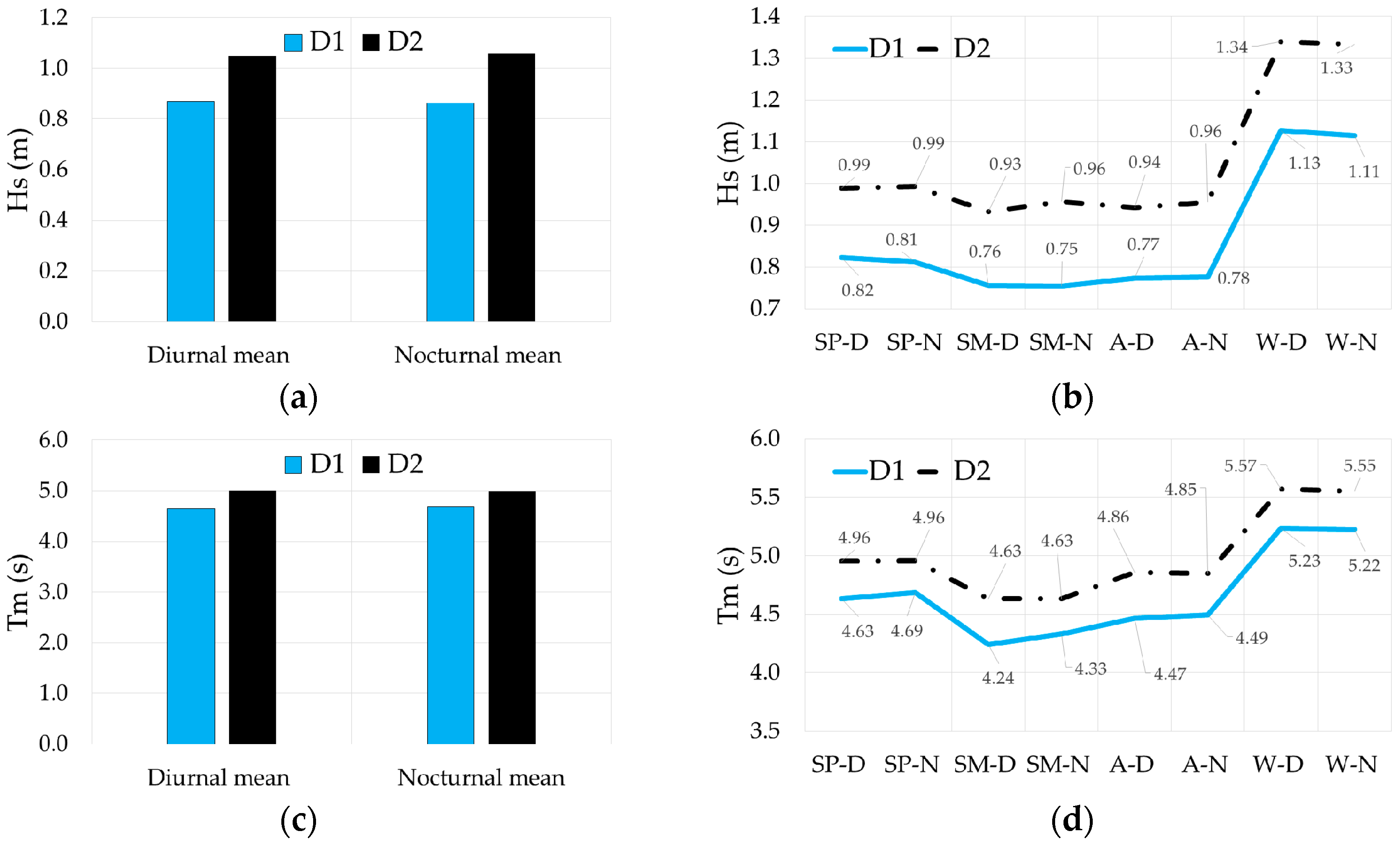
Figure 13.
Zone E, evaluation of the wave conditions considering the ECMWF data for the 11-year interval 2005–2015; (a) Hs mean values comparison of diurnal against nocturnal for total time; (b) Hs mean values comparison of diurnal against nocturnal for each season; (c) Tm mean values comparison of diurnal against nocturnal for total time; (d) Tm mean values comparison of diurnal against nocturnal for each season.


Figure 14.
Wind power density, annual average, diurnal mean, nocturnal mean and maximum mean for the 10 reference points considered.
Figure 14.
Wind power density, annual average, diurnal mean, nocturnal mean and maximum mean for the 10 reference points considered.

Figure 15.
Siemens SWT 3.6-120 wind turbine power curve.

Figure 16.
Assessment of the Siemens SWT 3.6-120 wind turbine performances. The results are based on the ECMWF data (2005–2015) and they are presented in terms of the mean values for: (a) capacity factor (%); (b) operating capacity (%); (c) rated capacity (%).
Figure 16.
Assessment of the Siemens SWT 3.6-120 wind turbine performances. The results are based on the ECMWF data (2005–2015) and they are presented in terms of the mean values for: (a) capacity factor (%); (b) operating capacity (%); (c) rated capacity (%).
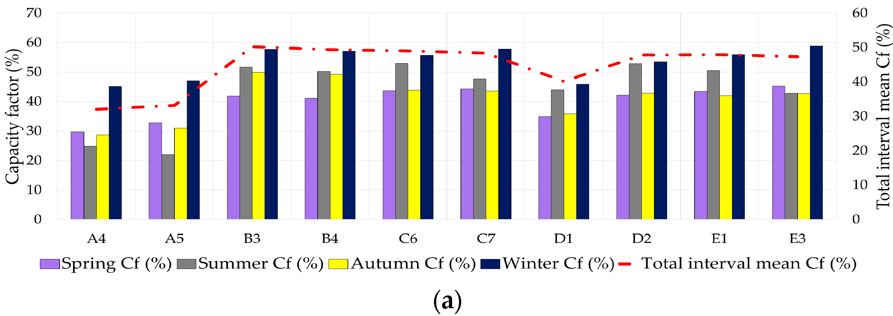
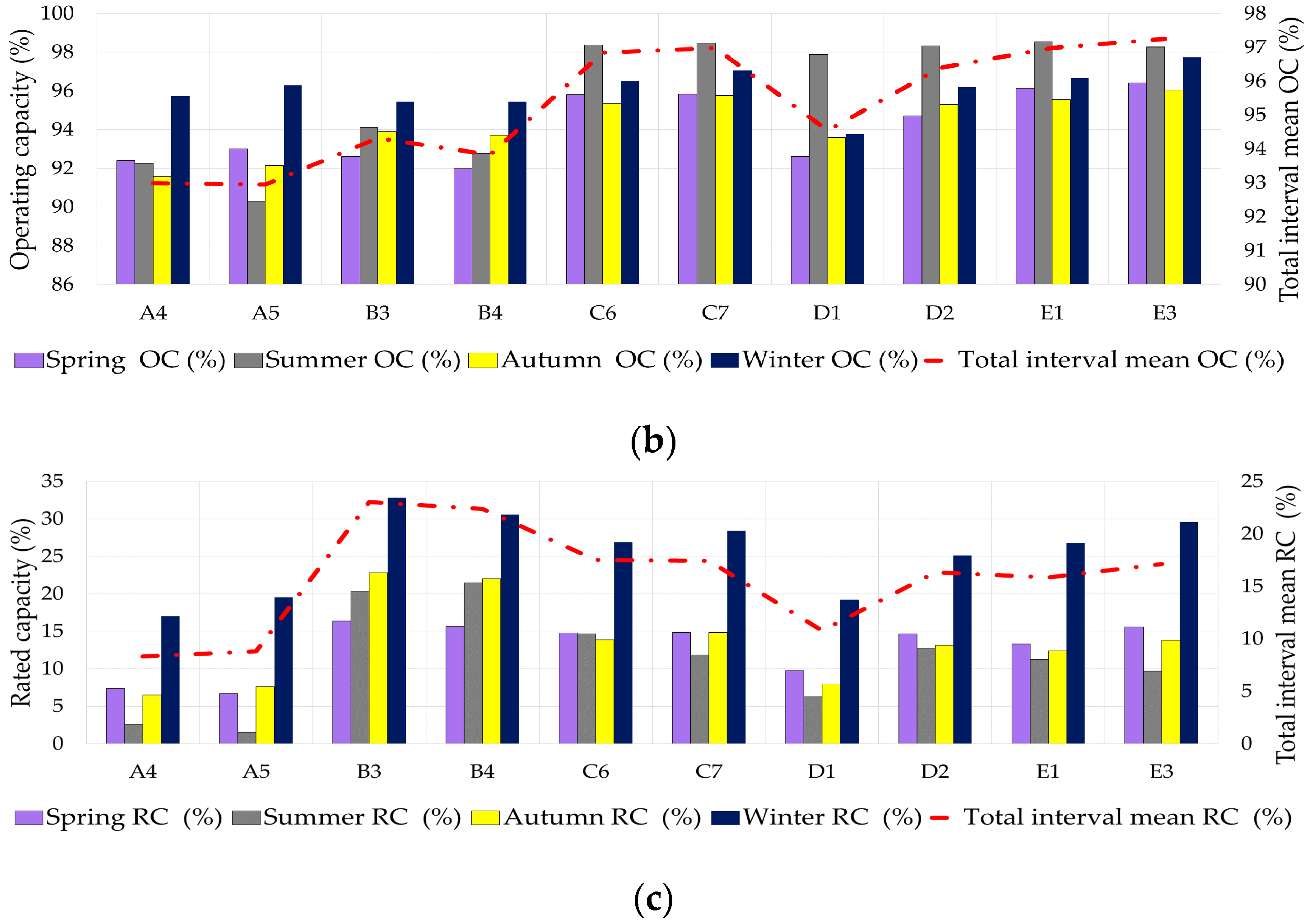
Figure 17.
Wave power density, Pwave, annual average, diurnal mean, nocturnal mean and maximum mean, for the 10 reference points considered.
Figure 17.
Wave power density, Pwave, annual average, diurnal mean, nocturnal mean and maximum mean, for the 10 reference points considered.

Figure 18.
Bivariate distributions corresponding to five reference points. ECMWF data processed for (a) point A5; (b) point B3; (c) point C6; (d) point D2; (e) point E3.
Figure 18.
Bivariate distributions corresponding to five reference points. ECMWF data processed for (a) point A5; (b) point B3; (c) point C6; (d) point D2; (e) point E3.


Table 1.
The geographical locations and the main characteristics of the points considered in the Ionian and Aegean seas.
Table 1.
The geographical locations and the main characteristics of the points considered in the Ionian and Aegean seas.
| Sea | Point | Latitude | Longitude | Depth (m) | Distance to Shore | |
|---|---|---|---|---|---|---|
| Proximity Island | (km) | |||||
| Ionian | A.1 | 39.63 | 19.71 | 62 | Kerkyra | 2.50 |
| A.2 | 38.46 | 20.52 | 79 | Kefallonia | 2.20 | |
| A.3 | 38.06 | 20.53 | 62 | Kefallonia | 3.74 | |
| A.4 | 37.68 | 20.76 | 86 | Zakynthos | 1.80 | |
| A.5 | 36.28 | 22.89 | 77 | Kythira | 1.92 | |
| Aegean | B.1 | 39.88 | 25.46 | 60 | Limnos | 8.00 |
| B.2 | 38.99 | 26.27 | 67 | Lesvos | 1.67 | |
| B.3 | 38.49 | 25.84 | 73 | Cios | 2.41 | |
| B.4 | 37.66 | 25.21 | 71 | Tinos | 2.70 | |
| B.5 | 37.28 | 24.87 | 98 | Syros | 8.80 | |
| B.6 | 37.44 | 26.57 | 90 | Patmos | 5.47 | |
| B.7 | 36.89 | 25.25 | 82 | Naxos | 14.00 | |
| B.8 | 36.84 | 26.94 | 88 | Kos | 7.00 | |
Table 2.
The geographical locations and the main characteristics of the points considered in the Crete, Levantine and Libyan seas.
Table 2.
The geographical locations and the main characteristics of the points considered in the Crete, Levantine and Libyan seas.
| Sea | Point | Latitude | Longitude | Depth (m) | Distance to Shore | |
|---|---|---|---|---|---|---|
| Proximity Island | (km) | |||||
| Crete | C.1 | 36.17 | 23.09 | 92 | Kythira | 3.56 |
| C.2 | 36.66 | 24.29 | 63 | Milos | 3.22 | |
| C.3 | 36.49 | 26.37 | 96 | Astypalaia | 2.39 | |
| C.4 | 36.13 | 27.68 | 89 | Rhodes | 1.93 | |
| C.5 | 35.57 | 27.06 | 73 | Karpathos | 1.49 | |
| C.6 | 35.34 | 26.31 | 87 | Crete | 2.27 | |
| C.7 | 35.48 | 25.22 | 89 | Dia | 1.34 | |
| C.8 | 35.71 | 23.73 | 95 | Crete | 2.00 | |
| Levantine | D.1 | 36.00 | 27.95 | 98 | Rhodes | 2.98 |
| D.2 | 35.35 | 26.95 | 92 | Kasos | 2.14 | |
| Libyan | E.1 | 35.01 | 25.95 | 96 | Crete | 2.20 |
| E.2 | 34.91 | 24.77 | 95 | Crete | 1.60 | |
| E.3 | 35.18 | 24.03 | 71 | Crete | 1.50 | |
Table 3.
Operational data and rotor information of Siemens SWT 3.6-120 wind turbine.
| Siemens SWT 3.6-120 | |||
|---|---|---|---|
| Operational Data | Rotor | ||
| Rated power (MW) | 3.6 | No. of blades | 3 |
| Cut-in wind speed (m/s) | 3 | Blade length (m) | 58.5 |
| Rated wind speed (m/s) | 12.5 | Rotor diameter (m) | 120 |
| Cut-out wind speed (m/s) | 25 | Swept area (m2) | 11,300 |
© 2017 by the authors. Licensee MDPI, Basel, Switzerland. This article is an open access article distributed under the terms and conditions of the Creative Commons Attribution (CC BY) license (http://creativecommons.org/licenses/by/4.0/).
Share and Cite
MDPI and ACS Style
Ganea, D.; Amortila, V.; Mereuta, E.; Rusu, E. A Joint Evaluation of the Wind and Wave Energy Resources Close to the Greek Islands. Sustainability 2017, 9, 1025. https://doi.org/10.3390/su9061025
AMA Style
Ganea D, Amortila V, Mereuta E, Rusu E. A Joint Evaluation of the Wind and Wave Energy Resources Close to the Greek Islands. Sustainability. 2017; 9(6):1025. https://doi.org/10.3390/su9061025
Chicago/Turabian StyleGanea, Daniel, Valentin Amortila, Elena Mereuta, and Eugen Rusu. 2017. "A Joint Evaluation of the Wind and Wave Energy Resources Close to the Greek Islands" Sustainability 9, no. 6: 1025. https://doi.org/10.3390/su9061025
Note that from the first issue of 2016, this journal uses article numbers instead of page numbers. See further details here.