
Optimization of Vehicle Routing Problem with Time Windows for Cold Chain Logistics Based on Carbon Tax


1
College of Mechanical Engineering, Chongqing University, Chongqing 400044, China
2
School of Transportation and Logistics, Southwest Jiaotong University, Chengdu 610031, China
3
Department of Management Engineering, Naval University of Engineering, Wuhan 430033, China
*
Author to whom correspondence should be addressed.
Sustainability 2017, 9(5), 694; https://doi.org/10.3390/su9050694
Submission received: 16 March 2017
/
Revised: 22 April 2017
/
Accepted: 24 April 2017
/
Published: 27 April 2017
(This article belongs to the Section Energy Sustainability)
Abstract
:In order to reduce the cost pressure on cold-chain logistics brought by the carbon tax policy, this paper investigates optimization of Vehicle Routing Problem (VRP) with time windows for cold-chain logistics based on carbon tax in China. Then, a green and low-carbon cold chain logistics distribution route optimization model with minimum cost is constructed. Taking the lowest cost as the objective function, the total cost of distribution includes the following costs: the fixed costs which generate in distribution process of vehicle, transportation costs, damage costs, refrigeration costs, penalty costs, shortage costs and carbon emission costs. This paper further proposes a Cycle Evolutionary Genetic Algorithm (CEGA) to solve the model. Meanwhile, actual data are used with CEGA to carry out numerical experiments in order to discuss changes of distribution routes with different carbon emissions under different carbon taxes and their influence on the total distribution cost. The critical carbon tax value of carbon emissions and distribution cost is obtained through experimental analysis. The research results of this paper provide effective advice, which is not only for the government on carbon tax decision, but also for the logistics companies on controlling carbon emissions during distribution.
1. Introduction
In recent years, the hot issue of greenhouse gas emission reduction has attracted close attention from all over the world [1]. At the United Nations Climate Conference in Copenhagen, China promised to reduce carbon emissions per unit of GDP to 50–60% of the 2005 level by 2020. In the global carbon emission statistics, transportation accounted for 14%, while the road transport carbon emission accounted for the entire transport sector carbon emission by up to 70% [2]. Cold-chain logistics is a high energy consumption and high carbon emission business in the logistics industry. Therefore, how to save energy and reduce carbon emissions in cold-chain logistics to seek a win-win situation of economic and environmental sustainability is a very serious problem, which is also a hot issue in the research of cold-chain logistics. The Chinese government also proposes that the national carbon market will be launched in 2017 and the comprehensive implementation of carbon emission trading system will be achieved by 2020. Thus, it is imperative to develop a carbon tax standard that can truly play a leading role of low-carbon green for a long time [3].
VRP was first proposed by Dantzig and Ramser [4] in 1959, and since then many research results have been produced on this classical optimization problem: the study by Desrochers and Verhoog [5] revealed a hybrid vehicle routing model; the concept of service time window was introduced in VRP study by Solomon and Desrosiers [6]; based on service time window constraints, Jabali et al. [7] considered the penalty cost, thereby obtaining the VRP model with soft time windows; Moghaddam et al. [8] added the uncertain demand factors to the VRP model; and Cattaruzza et al. [9] discussed vehicle routing problem with multiple trips. There are also a large number of research results on the VRP model algorithm: for example, the accurate algorithm includes the branch and bound method proposed by Laporte et al. [10], dynamic programming algorithm studied by Righini et al. [11], cutting plane method introduced by Kallehauge [12], etc.; and the heuristic algorithm is divided into saving algorithm [13], two-stage algorithm [14], tabu search algorithm [15] and so on.
Some scholars believe that the traditional VRP model should not only consider the economic benefits, but also think about the reduction of carbon emissions from the social and environmental aspects [16]. Carbon emission factors were introduced by Li et al. [17] to establish a low-carbon path model, and they designed an improved tabu search algorithm for research; the VRP model and the carbon emission model were constructed by Palmer [18], which mainly analyzed the influence of velocity on the carbon emission, but the influence of the vehicle load was missed; Maden et al. [19] putted forward a VRP model with time window and solved it with an improved heuristic algorithm, which could achieve 7% reduction in carbon dioxide emissions; and, considering the factors of carbon emissions, the VRP model for reducing fuel consumption was constructed by Kuo [20], and an improved simulated annealing algorithm was used to solve the problem.
In this paper, the research of VRP model is limited in the scope of the cold chain logistics in China. In this area, there are a series of research results: Yang et al. [21] studied the VRP model of perishable goods in cold chain logistics, and used a genetic algorithm to optimize the distribution paths; Zhang et al. [22] proposed an multi-depot and multi-vehicle routing problem model and elite selection based on Partheno-Genetic algorithm; and Ma et al. [23] studied the vehicle routing optimization model of cold chain logistics based on stochastic demand. In addition, the Non-Chinese scholars have also carried out much research on cold chain logistics VRP. Tarantilis et al. [24] took the fresh meat and milk of Greece as an example, and the threshold algorithm was introduced to optimize the distribution path of the VRP model. For a real distribution problem faced by a cold chain logistics enterprise in Portugal, a VRP model with multiple constraints was proposed by Amorim et al. [25].
The existing literature can be divided into three categories according to the differences of the study scope: general logistics VRP study without considering carbon emission, ordinary logistics VRP considering carbon emission and cold chain logistics VRP without considering carbon emission. However, the research results of VRP in cold chain logistics considering carbon emission factors are relatively few. In addition, the influence of the energy consumption of refrigeration equipment on carbon emissions is often ignored. Besides, few studies have considered path optimization based on carbon taxes. Based on the above analysis, this paper aims to deal with optimization of VRP with time windows for cold chain logistics based on carbon tax. Since changes in energy consumption can affect carbon emissions, we consider whether the door of refrigerated truck opens leads to different energy consumption in the transport process and unloading process. Then, a green and low-carbon cold chain logistics distribution route optimization model with minimum cost is constructed. Taking the lowest cost as the objective function, the total cost of distribution includes the following costs: the fixed costs which generate in distribution process of vehicle, transportation costs, damage costs, refrigeration costs, penalty costs, shortage costs and carbon emission costs.
This paper further proposes the CEGA to solve the model. The CEGA can quickly and effectively seek the optimal solution of the model. We combine two kinds of operators, inversion mutation and insertion mutation, in the genetic algorithm to form the combined operator of CEGA, and then, the approximate optimal solution is obtained. Meanwhile, a large number of experiments are carried out by setting different carbon tax values and the critical interval values of carbon emissions and optimal path is obtained, which provides some planning suggestions for the reasonable control of carbon emissions during distribution.
2. Model Formulation
2.1. Problem Description
With the rapid development of China’s urbanization, fresh and frozen food consumption of urban and rural resident increases year by year, but the cold chain logistics facilities such as cold storage, refrigerated trucks etc. are insufficient. Under the background of low-carbon economy, how to make good use of limited resources to plan cold chain logistics distribution is an urgent problem to be solved. The VRP model of cold chain logistics considering carbon footprint in this paper can be described as follows: we focus on the vehicle routing problem with a central depot, denoted by “”, and a set of customers {} to be serviced, a depot of cold-chain logistics () distributes products to different customers through k refrigerated trucks. The locations of the depot and each customer are known. Besides, each refrigerated truck will return to the depot after the distribution task has been completed. We build a low-carbon cold chain logistics distribution route optimization model with minimum cost. Meanwhile, there are the fixed costs which generate in distribution process of vehicle, transport costs, damage costs of fresh agricultural products, cooling costs and the cost of carbon emissions need to be considered. In addition, customer demand and the constraints of the vehicle load must be met. Then, we hope to obtain the vehicle distribution plan with the smallest possible carbon emission under the premise of ensuring the delivery services are completed.
2.2. Problem Assumptions
In China’s vast rural areas, administrative regions are often divided by the influence of geographical factors and population density. In an administrative area, in general, administrative center with a relatively good economy and infrastructure has the ability to build a cold chain logistics distribution center (i.e., depot). The VRP model of cold chain logistics in this paper can be assumed as follows: a cold chain logistics company uses the single type of refrigerated vehicle responsible for the distribution tasks in the entire administrative region. In addition, in order to maintain the reasonable and scientific nature of the hypothesis, the mathematical models in this paper are supported by literature reference. We refer to References [17,23,26], and make the following assumptions:
- (1)
- There is only one type of refrigerated truck. Furthermore, the load capacity of refrigerated truck is known, and the total customer demand on each route cannot exceed the vehicle capacity.
- (2)
- There is no situation of receiving in the distribution process. The task of refrigerated truck is only delivery.
- (3)
- During the delivery, the refrigerated truck runs at a uniform speed and the fuel is diesel.
- (4)
- The demand of each customer must be satisfied, and is only visited once.
- (5)
- In this paper, CO2 emission is the only factor to be considered when considering greenhouse gas emissions.
2.3. Parameters and Variables
According to the needs to build the model, this paper sets the following parameters:
- n: The number of customers that the depot needs to serve.
- K: The number of refrigerated truck owned by the depot.
- Q: The maximum load capacity of refrigerated truck.
- P: The price of the unit commodity.
- : Fixed cost of refrigerated truck k.
- : The distance between customers i and j.
- : The cost of per kilometer when the refrigerated truck k driving from customer i to customer j.
- t: The delivery time required for distribution.
- : The spoilage rate of product.
- : The number of products remaining on board when the refrigerated truck leaving customer i.
- : The time required for a refrigerated truck to serve customer i.
- : The demand of customer i.
- : The refrigeration costs which generate during transportation process of unit time.
- : The refrigeration costs which generate during unloading process of unit time.
- : The unloading time which is needed when refrigerated truck k serves the customer i.
- : The traveling time of the refrigerated truck k from the customer i to the customer j.
- : The time point when the refrigerated truck k reaches the customer i.
- : The unit cost of shortage of cold chain product.
- : The cost of waiting for the unit time if refrigerated truck arrives at customer node in advance.
- : The cost of punishing for the unit time if refrigerated truck is late to the customer node.
- : The time window that the customer i expects to be served.
- : The service time window that the customer i can accept.
- : The actual load of refrigerated truck k.
- : The actual demand of the customer nodes that the refrigerated truck k serves.
- : The fuel consumption of per unit distance when the vehicle is running.
- : The fuel consumption of per unit distance when the vehicle is fully loaded.
- : The fuel consumption of per unit distance when the vehicle is empty.
- : The load capacity of the refrigerated truck when it travels between customer i and customer j.
- : The coefficient values of CO2 emission.
- : The carbon emission that generate from distributing unit weight cargoes during driving unit distanc .
- : The carbon tax of per unit of carbon emissions.
- is a 0–1 variable, if the vehicle k of depot is used, otherwise .
- is a 0–1 variable, if the vehicle k passes the road between customer i and customer j, otherwise .
- is a 0–1 variable, if the vehicle k services for customer i, otherwise .
2.4. Mathematical Model
The cold chain logistics VRP in this paper belongs to a type of vehicle routing problem. The VRP model of cold chain logistics considering carbon footprint is proposed to realize the path selection of low-carbon distribution. Carbon emissions in the process of cold chain distribution generate from the vehicles fuel consumption as well as from refrigeration equipment. If we only put the minimum carbon emissions as the optimization goal, it is pointless for logistics enterprises. Therefore, the objective function is not to minimize the carbon emissions or fuel consumption, but to use comprehensive cost minimum as objective function when we establish the mathematical model.
The costs of optimization mainly include: the fixed costs which generate in distribution process of vehicle, transportation costs, damage costs in the process of distribution, refrigeration costs, penalty costs, shortage costs and carbon emission costs.
2.4.1. The Optimization Goal Setting
(1) The fixed costs of vehicles
When dispatching each refrigerated truck to carry out the distribution task, some fixed costs need to be paid, including the cost of buying or renting refrigerated trucks, the driver’s wages, refrigerated trucks fixed losses and so on. The fixed costs of using a vehicle are usually constant which mainly refers to the fixed cost of vehicles with delivery tasks, except idle vehicles. Additionally, it is not related to the vehicle mileage and the number of customers.
Assuming that the depot has a total number of m delivery routes, that is, m refrigerated trucks will be required to provide distribution services for n customer nodes, represents the fixed costs of vehicle k. The fixed costs can be expressed as:
(2) Transportation costs of vehicles
This section considers only transportation costs; the cost of refrigeration in transit will be analyzed separately in the following. In view of the present situation of urban and rural cold chain logistics distribution in China [27], the transportation costs of vehicles are influenced by fuel consumption, maintenance and other factors, and it is proportional to the vehicle mileage. The transportation costs of the refrigerated vehicle can be expressed as:
(3) The damage costs
Different from the ordinary VRP, cold chain VRP transport products are perishable goods. The general VRP model considers the damage of goods during loading and unloading, which may be due to the loss caused by collision. However, this paper considers that the damage costs of perishable products are mainly due to changes in temperature during the transport and handling of the goods. There is a characteristic of perishable in refrigerated goods, so the temperature, humidity, concentration of oxygen in storage environment, moisture content in the product and other factors will affect the change of quality. The quality of perishable goods will gradually decline or even lose its value with the extension of time and temperature changes. When the quality of the product declines to a certain extent, there will be damage costs. The amount of remaining goods in refrigerated trucks is not only closely related to the demand of customers, but also directly related to the loss of the goods in the process of cold chain logistics distribution [23].
In this paper, we introduce the variable function of refrigerated goods quality [28]: where is the quality of the product at time t; t is the transportation time of the product; is the quality of the product from the depot; and is the spoilage rate of the product, its value is related to the characteristics of fresh agricultural products and temperature. It is assumed that in the process of transportation the temperature of product environment is invariable, so the spoilage rate of fresh agricultural products can be considered as a constant in an invariable temperature, the quality of fresh agricultural products with time showing characteristics of exponential change. For the same kind of products, the higher storage temperature then the spoilage rate will be larger if other factors remain unchanged. The value of is an increasing function of temperature, i.e. it increases with temperature.
Hence, when the vehicle is starting from the depot to the customer i and the door is not opened in the process of transportation, the damage costs can be expressed as:
where P is the unit price of the distribution products; is the demand of customer i; represents the time point when the refrigerated vehicle k reaches the customer i; represents the departure time of the vehicle k from the depot; indicates the spoilage rate of the product at a particular temperature during the transport process; and is a 0–1 variable, if the vehicle k services for customer i, otherwise .
When the door is opened, due to the convection of air, the temperature inside the vehicle will rise, and the spoilage rate of fresh agricultural products will change accordingly. The hypothesis of this spoilage rate is (), when the vehicle arrives at the customer i, the damage costs generated by opening door in the process of unloading can be defined as:
where represents the number of products remaining on board when the refrigerated vehicle leaves customer i; and is the time required for a refrigerated vehicle to serve customer i.
Therefore, we can get the total damage costs in the entire distribution process. is the sum of and .
(4) The refrigeration costs
Different from ordinary VRP, the refrigeration costs should be considered in the transportation of cold chain VRP model. Because of the difference of refrigeration mode, refrigerated vehicles are divided into three types: mechanical refrigeration, cold storage plate cooling and liquefied gas refrigeration. Presently, refrigerated vehicles of mechanical refrigeration are the main refrigerated vehicles in China [29]. Refrigeration costs include the cost caused by energy consumption of the vehicle in order to keep the low temperature during delivery, as well as the cost of additional energy supplied by the refrigeration system during the unloading process.
Thus, in the process of transportation, vehicle refrigeration costs as follows:
During the unloading process, the refrigeration costs of refrigerated vehicles as follows:
Thus, the total refrigeration costs are :
where represents the waiting time of refrigerated vehicle k for non-unloading when servicing customer j.
(5) The penalty costs
In the distribution, customers generally have a time limit for the distribution of chilled or refrigerated foods. If the goods do not reach the destination within the time period agreed by the customer, it will affect customer satisfaction, increase vehicle energy consumption, bring goods loss costs and so on, and then produce the corresponding penalty costs. Thus, the concept of time window and Vehicle Routing Problem with Time Windows (VRPTW) are introduced. The time window is divided into hard time window and soft time window. In this paper, combining the actual situation of China’s urban and rural distribution [30], we choose to calculate the penalty costs of soft time window as follows:
where represents the time of arriving in advance when the vehicle k services customer i; and represents the late time of the vehicle k services customer i.
(6) The shortage costs
Many uncertain factors (similar to the loading and unloading cargo damage, etc.) cause the actual total demand of customers over the actual load of refrigerated vehicle in the distribution process, which will lead to customer needs unable to be met, and then producing shortage costs. Meanwhile, the quality of service will also be affected.
The shortage costs in the distribution process can be expressed as:
(7) The carbon emission costs
As mentioned above, the refrigeration method used in Chinese refrigeration vehicles is mainly mechanical refrigeration. The energy consumption of mechanical refrigeration also affects the amount of CO2 emissions. After a comprehensive study of the literature [31,32,33,34], the carbon emissions in the cold chain distribution process mainly include two aspects: the generation of fuel consumption and the energy consumption of refrigeration equipment.
For the amount of CO2 emissions from fuel consumption in the distribution process, this paper uses the formula to express: Carbon emissions = fuel consumption × CO2 emission coefficient [35]. This part of the fuel consumption is not only related to the transport distance, but also influenced by the vehicle load capacity and other factors. Some scholars have collected relevant statistical data for regression analysis to get the fuel consumption in unit distance can be expressed as a linear function that depends on the number of goods carried by vehicle X [36]. As a result, if the total vehicle weight is divided into vehicle weight and the number of goods carried by vehicle X, the unit distance fuel consumption can be expressed as:
It is assumed that the maximum load capacity of the vehicle is , the fuel consumption of per unit distance at full load is , and the fuel consumption of per unit distance is when vehicle is empty. From the above equation, and can be, respectively, calculated as follows:
Thus, can be expressed as:
Thus, the unit distance fuel consumption can be expressed as:
Therefore, the carbon emissions generated when the vehicle travels between customer i and customer j can be expressed as:
where is the load capacity of the refrigerated vehicle when it travels between customer i and customer j; represents the unit distance fuel consumption when the number of goods carried by the vehicle is ; and is the coefficient value of CO2 emission.
The CO2 emissions generated by the refrigeration equipment in the distribution process are also related to the transportation distance and the amount of cargo carried. If cargo is transported from the customer i and customer j, the carbon emissions generated due to refrigeration when the vehicle travels between customer i and customer j can be expressed as:
where represents the carbon emissions that generate from distributing unit weight cargoes during driving unit distance .
The distribution vehicle is empty in the process of returning to depot when it completes the distribution task for all customers, so the refrigeration is not needed at this time, and there are no carbon emissions generated by refrigeration. The source of carbon emissions is only vehicle fuel consumption in the process of returning to depot, and can be expressed as according to Equation (16).
Thus, the CO2 emissions generated during the entire distribution process are as follows:
This paper introduces carbon tax mechanism to calculate carbon emission costs, that is carbon emission costs = carbon tax × carbon emission. If the carbon tax is , the total carbon emission costs in distribution process can be expressed as:
2.4.2. Optimize Model Settings
Through the comprehensive analysis of seven optimization objectives of costs, vehicle fixed costs, transportation costs, damage costs, refrigeration costs, penalty costs, shortage costs and the costs of carbon emissions in Section 2.4.1, the VRP model of cold chain logistics considering the carbon footprint is given by the following:
Subject to
It indicates the objective of our problem is to minimize the sum of costs in Objective Function (20). Constraint (21) represents that there is a total of k refrigerated trucks in the depot, and each customer has only one refrigerated truck for distribution services. The total number of customers is n that need the depot to provide services, as mentioned in Constraint (22). Constraint (23) shows that the demand of all customers met by vehicle k in a route does not exceed the maximum capacity of vehicle k. Constraint (24) imposes the notion that, the refrigerated trucks which are starting from the depot must return to the depot after they have served their customers. The number of routes constraint is controlled by Equation (25) to ensure the number of paths must be less than or equal to the number of refrigerated vehicles owned by the depot. Refrigerated trucks maintain service continuity for two customer nodes, which is imposed by Constraint (26).
3. Algorithm Design
The CEGA is proposed to solve the model in this paper. CEGA simulates the natural evolutionary process of “evolution-degradation” in catastrophism theory, and shows the characteristic of cyclical reciprocation [37]. At the same time, a combination operator [38] is designed to ensure the algorithm can get the optimal solution; that is, the evolution of the algorithm evolves toward the direction of the optimal value of the fitness function. This operator has the feature of keeping the evolution trend of the population to ensure that the periodicity of the CEGA is not a simple reciprocation, but presents a spiral rising characteristic in the general trend.
The design of CEGA for an evolutionary cycle is as follows: firstly, the combination operator is used as an algebra that is designated by genetic operator for population evolution; secondly, the population is reconstructed under the condition of reserving the best individual in history; and, finally, a generation evolution is conducted on individuals in the population according to the adaptive selection of crossover probability and mutation probability, which will cause a temporary degradation in the population (the average fitness of the population is decreased), and then transferring to the next evolutionary period. Through a number of such evolutionary cycles, CEGA will finally find the optimal solution.
The detailed steps are as follows:
(1) Coding
Natural number coding method is used to encode chromosomes in this paper. The number of vehicles dispatched, the number of customers served by per vehicle, and the order of service are the primary decision variables for the model. Thus, the chromosomes are encoded by the corresponding arrangement coding method of vehicles and the customers, and each chromosome represents a solution. VRP is mainly to determine the number of distribution paths (corresponding to the number of vehicles), the number of customers and customer service order in each distribution path. Detailed ideas are given by the following:
When developing a vehicle permutation expressed by m natural numbers (the natural numbers can be repeated, ) and a customer permutation denoted by n natural numbers that do not repeat (), these two permutations correspond to each other and then a solution is formed, the solution is a distribution path scheme.
For example, three refrigerated vehicles are used to deliver goods for nine customers, assuming there is a solution (472365189) and (111222333), the permutation is as Figure 1 shows.
In this example, the vehicle 1 provides service for customers 4, 7, and 2; customers 3, 6, and 5 are served by vehicle 2; and vehicle 3 serves customers 1, 8, and 9. The corresponding sub-paths can be described:
- Sub-path 1: 0-4-7-2-0
- Sub-path 2: 0-3-6-5-0
- Sub-path 3: 0-1-8-9-0
The problem can be disintegrated through this coding and arrangement method, which will reduce the complexity of the problem.
(2) Generating feasible initial population at random
Genetic algorithm starts from the population of the problem solution to search, so it is necessary to generate an initial population consisting of numerous individuals as the starting point of evolution. What mainly needs to be determined in the generation process of initial population is the size of population and the population size refers to the number of individuals in the population. The operation performance of the genetic algorithm will directly be affected by the population size. On the one hand, the sample size is not enough if the scale is too small, which will lead to a bad search result. However, there is huge computation if the scale is too large and the convergence rate will be slowed. We get an initial population which scale is N using a stochastic approach. N different chromosomes as described above are generated to form the first population accord with the initial population scale.
(3) Determining fitness function and fitness calculation
The higher the fitness of an individual, the better the performance of the individual, but the objective function of the low-carbon cold chain distribution path optimization problem in this paper is the least cost, so we take the reciprocal of the objective function value as the fitness of the individual, which can be expressed as:
where represents the fitness of individual i, and represents the objective function value corresponding to individual i.
(4) Selection strategy operation
Selection is the process of selecting the best individuals from the current population to produce a new population. We use the tournament selection strategy [39] to select in this paper, which can guarantee better individuals are selected with higher probability and worse individuals are eliminated, which make the algorithm converge quickly. Meanwhile, the phenomenon of precocity can be avoided effectively, so that the population can maintain diversity. The principle of this method is selecting based on the size of individual fitness value; that is, selecting some individuals randomly from the population and then the individual who has the highest fitness value will be selected into offspring population. This operation is repeated until the size of new population is identical to the original population size.
(5) Crossover operation
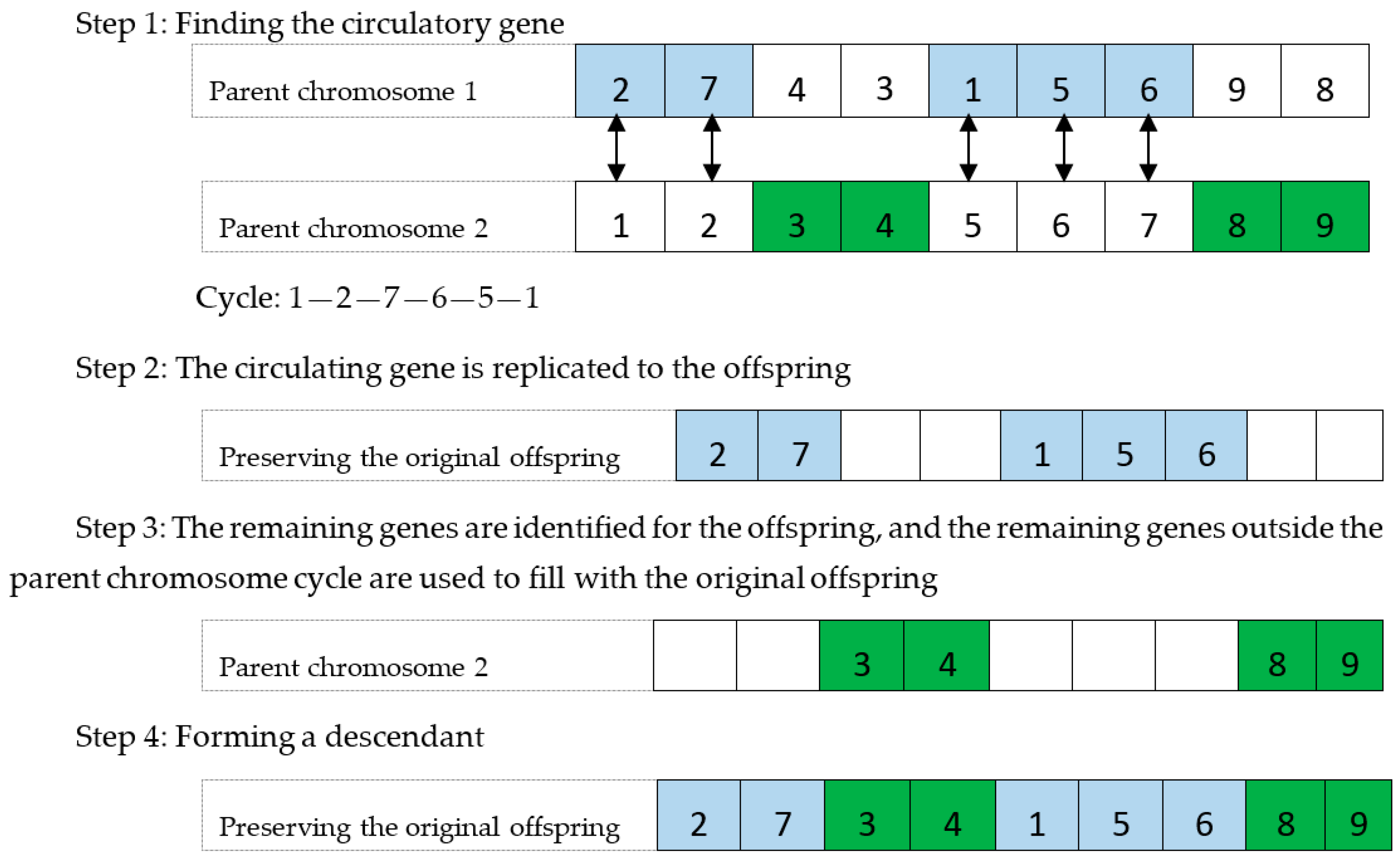
Crossover operation is to select individuals in a population with a certain crossover probability, and then replacing and recombining some genes of two parents to generate new individuals [40]. Cycle crossover is chosen to cross and recombine to form new populations, which is explained as follows: first, according to the corresponding gene position of the parent chromosome, a cycle will be found; then, a gene on the parental chromosome cycle is replicated to a descendant chromosome; and, finally, the genes that have been circulated on the other parent chromosome are deleted, and filling the remaining positions of the offspring with the remaining genes. Examples of cycle crossover procedures are shown as Figure 2.
(6) Mutation operation
Mutation operator is a gene mutation that mimics the evolution process of organism. In the genetic algorithm, the mutation operator can avoid the local search and increase the diversity of the population to some extent. There are some common mutation operators including inversion mutation, insertion mutation, inter change mutation and so on. We adopt three kinds of mutation at the same time in the paper; the specific mutation strategies are as follows:
Inversion mutation: Two reversal points are randomly selected in the coding string, and then the inverted sequence of the genes between the two reversal points is inserted into the original position. As shown in Figure 3, 3 and 6 are chosen as the reversal points; the genes are reversed to insert into the original position; and then the gene sequence between 3 and 6 is changed.
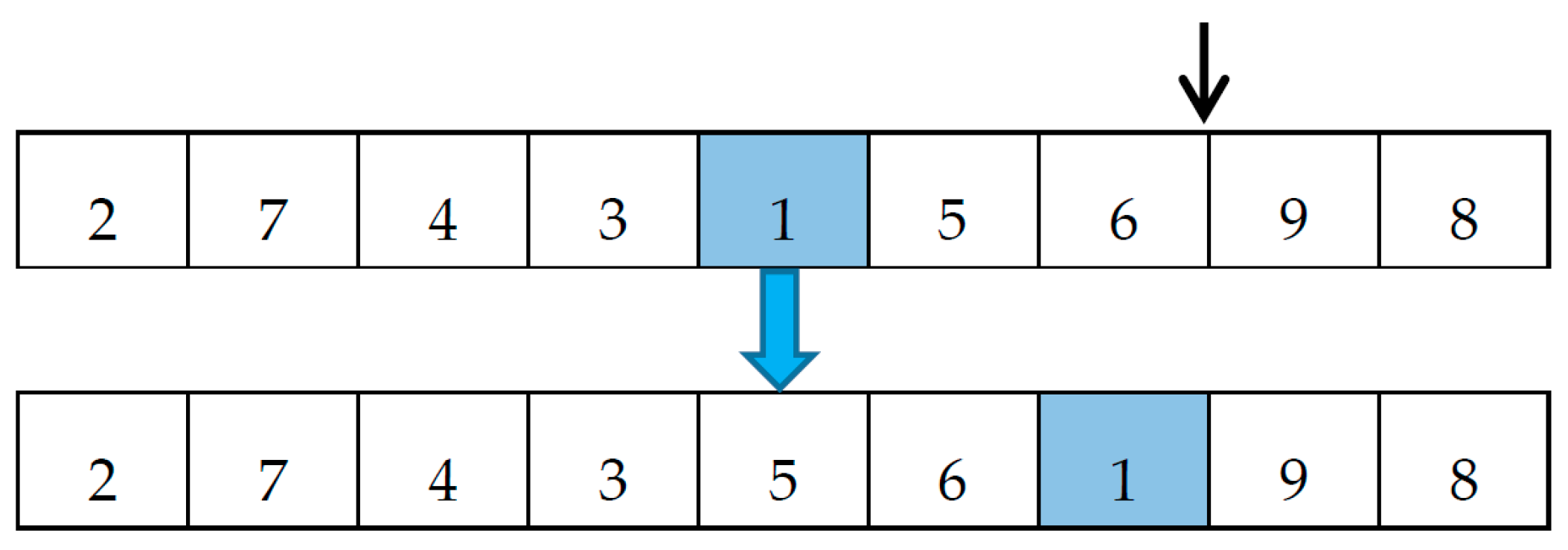
Insertion mutation: As shown in Figure 4, we randomly select gene 1 in the parent coding string, randomly select an insertion point 9, and then insert 1 in front of 9.
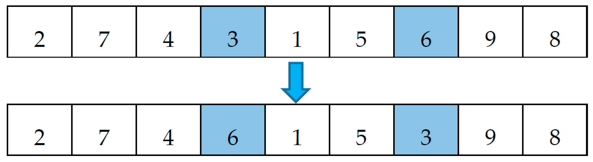
Interchange mutation: Two exchange points are randomly selected in the coding string, and then exchange the location of these two exchange points. As shown in Figure 5, we select exchange points 3 and 6, which will become 6 and 3 after the interchange mutation.
We combine the inversion mutation operator and insertion mutation operator in order to ensure the strategy of algorithm evolutionary trend generates heredity, which is the combination operator of the CEGA mentioned above. The fitness value of the sub-individual is calculated when the combination operator is executed. In addition, the interchange mutation is mainly used outside the iterative cycle of CEGA, which performs genetic operation according to the adaptive crossover probability. The three kinds of mutation operators aim at the customer code, so the corresponding vehicle code should be adjusted accordingly after the mutation of the client code, and the fitness value of the corresponding chromosome should be modified.
(7) Producing a new generation population
A new generation population will be generated by selecting strategies, crossover operations and mutation operations.
(8) Terminating condition
The termination criterion is a condition for determining whether or not to stop the operation. The algorithm terminates when the number of evolutionary cycles is greater than the maximum number of evolutionary cycles, otherwise, it will continue to evolve until the number of evolutionary cycles reaches the specific maximum. Here, the termination criterion we choose is to reach the pre-set evolutionary generation.
(9) Decoding
Evolution will be stopped if the pre-set evolutionary generation is reached. In the last-generation population, the corresponding distribution paths of individuals with the best fitness value are selected; as a result, we can get the distribution plan that is the approximate optimal solution of the low-carbon cold chain VRP model.
4. Experimental Design and Results
In this section, we use an example experiment to solve the algorithm we designed. The changes in carbon emissions, carbon emission costs, and total costs at different carbon tax levels are analyzed. Section 4.1 describes the example of experimental problems in this paper and the design of the parameters of the model and algorithm. The experimental results are analyzed in Section 4.2.
This paper uses MATLAB R2014a to implement the proposed algorithm, and all experiments in this paper are evaluated on PCs with Intel® Core™ (Santa Clara, CA, USA) i7-3610QM CPU@ 2.10 GHz 2.10 GHz and memory of 4 GB.
4.1. Description of Experimental Problems and Parameter Setting
4.1.1. Experimental Data and Parameter Settings
We use the data in Reference [30] and choose 20 supermarket stores as the solution clients in the case. The location, demand, and service time window of each customer are shown in Table 1; the parameters of the refrigerated vehicles are shown in Table 2; and the parameter settings of the model are in Table 3. The depot uses road transportation to deliver goods, and the same type of vehicle is adopted to provide services to customers. Furthermore, all roads are non-forbidden road. The average speed of distribution vehicles is 25 km/h in the distribution process, 3 Yuan/km is transportation cost in per unit mileage, fixed cost of per vehicle goes to 200 Yuan, and the goods loaded in each vehicle weigh a maximum of 9 tons.
4.1.2. Parameter Setting for CEGA
The parameter setting for the CEGA has a considerable influence on the algorithm’s ability to solve the problem, thus affecting the results of the model. A better solution can be obtained through the appropriate number of generations and the mutation probability [26]. We refer to the algorithm parameter setting in References [26,41,42,43], and, according to the software running speed of solving the model example proposed in this paper, the parameters are set as follows: the number of generations is 5000; the mutation probability is 0.05; 10 is set as the number of iterations of an evolution period; the initial test population is 100; and we use 0.4 to be the crossover probability.
4.2. Analysis of Experimental Results
We refer to carbon taxes in developed and developing countries, and set the value of carbon tax from 0 to 90 in the model and get solutions [44]. The carbon emissions, carbon emission costs, and the total costs under different carbon tax will be obtained by decoding the optimal solution in the last iteration cycle. The experimental results are shown in Table 4.
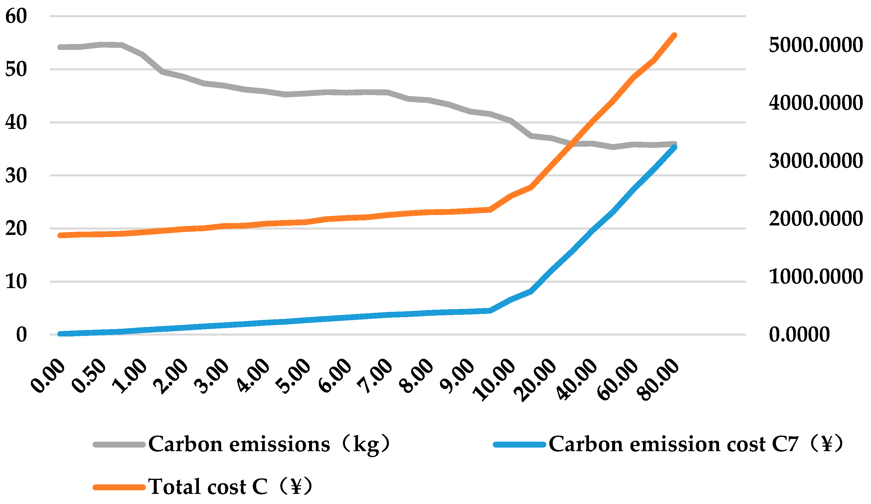
Based on the data analysis, we get the curve of carbon emissions, carbon emission costs and total cost under different carbon tax.
Inference I: The carbon emission costs and the total cost of distribution increase with the rise of carbon tax. In this example, the carbon emission costs and the total cost of distribution C will change as gradually increase when ;
Inference II: When the carbon tax is less than a critical point (we assume that the critical value is CR1), the change in the carbon tax has no effect on carbon footprint, thus there is no impact on the distribution path planning. In Figure 6, we can conclude that, in this example, CR1 = 1, the carbon footprint tends to be stable when ;
Inference III: When the carbon tax is more than a critical point (we assume that the critical value is CR2), the change in the carbon tax has no effect on carbon footprint, thus there is no impact on the distribution path planning. In Figure 6, we can conclude that, in this example, CR2 = 40, carbon footprint will not decrease with the increase in carbon tax when ;
Inference IV: The increase of carbon tax will bring about the decrease of carbon footprint in a certain range (). In this example, carbon emissions gradually reduce with the increase in when .
Clearly, as can be seen in Table 4 and Figure 6, we know that inference I is correct. Next, we will verify inferences II, III and IV.
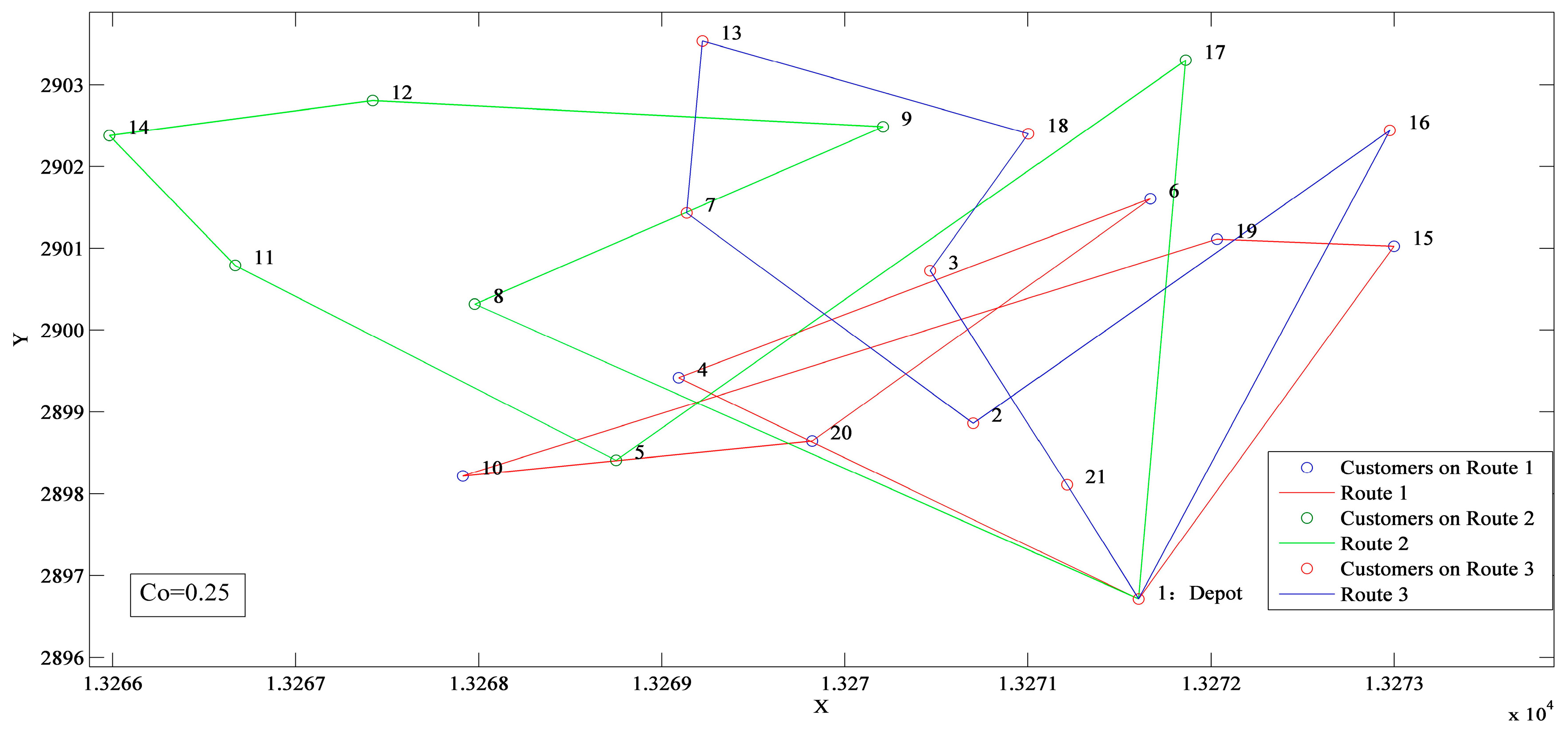
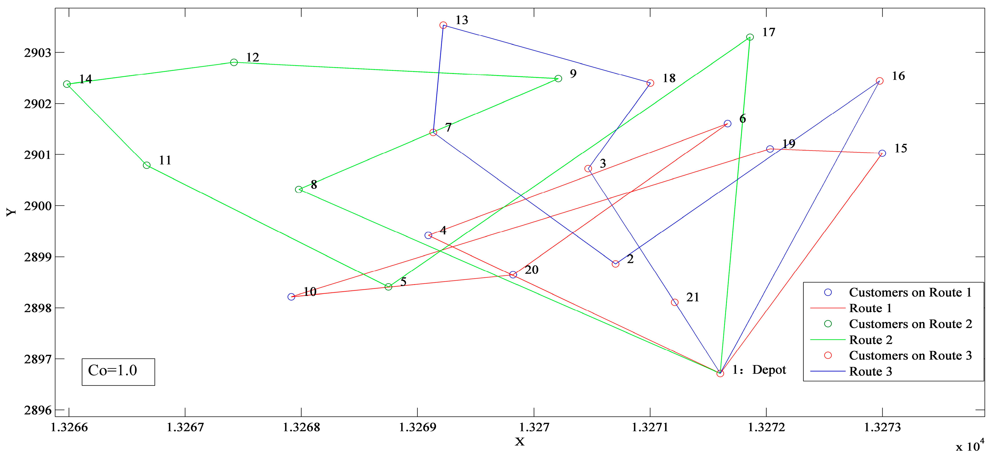
In order to verify inference II, is set to be 0.1, 0.2, 0.3, …, 1.0 for 10 groups of experiments. Each group of data is taken into the model to solve ten times, and then the optimal solution that has optimal fitness value and the optimal distribution path in each group can be selected. The same ten sets of data have the same results, which proves that the optimal distribution path does not change. When is set to 0.25, 0.5, and 1.0, the optimal distribution paths obtained by solving the model is shown in Figure 7, Figure 8 and Figure 9.
We obtained the same distribution plan through Figure 7, Figure 8 and Figure 9. The change in the carbon tax has no effect on the distribution path planning. The distribution task requires three vehicles to complete, and the distribution service order is shown in Table 5.
In order to further validate inference II, we analyze the proportion of fixed costs of vehicle , transportation costs , damage costs , refrigeration costs , penalty costs , shortage costs and carbon emission costs in the total cost of distribution C when is set to 0.25, 0.5, and 1.0 . The cost proportion analysis is shown in Table 6, Table 7 and Table 8.
As shown in Table 6, Table 7 and Table 8, the proportion of carbon emission costs () in the total cost of distribution is too low. Therefore, the carbon emission costs has no significant effect on the total cost of distribution, thus there is no change on path planning when , and this result further supports inference II.
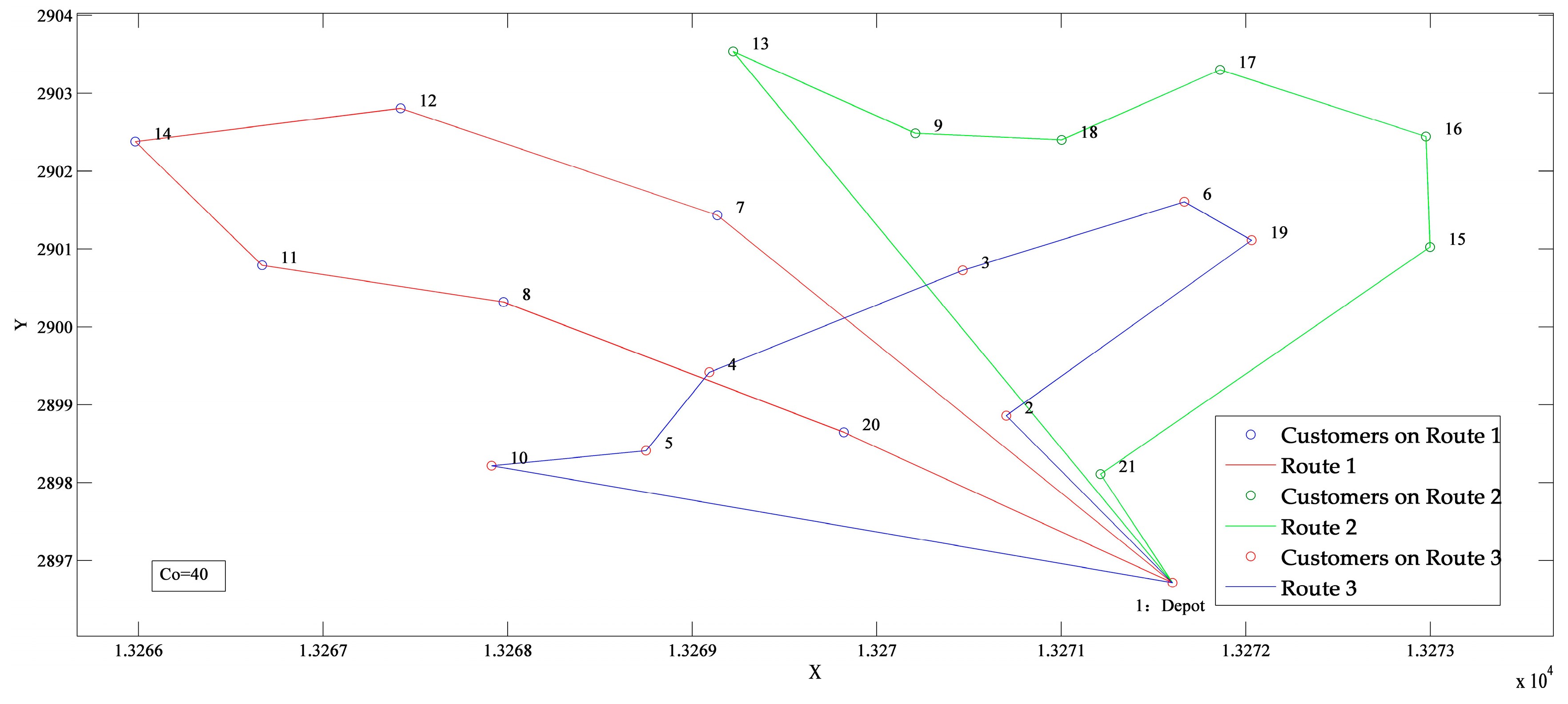
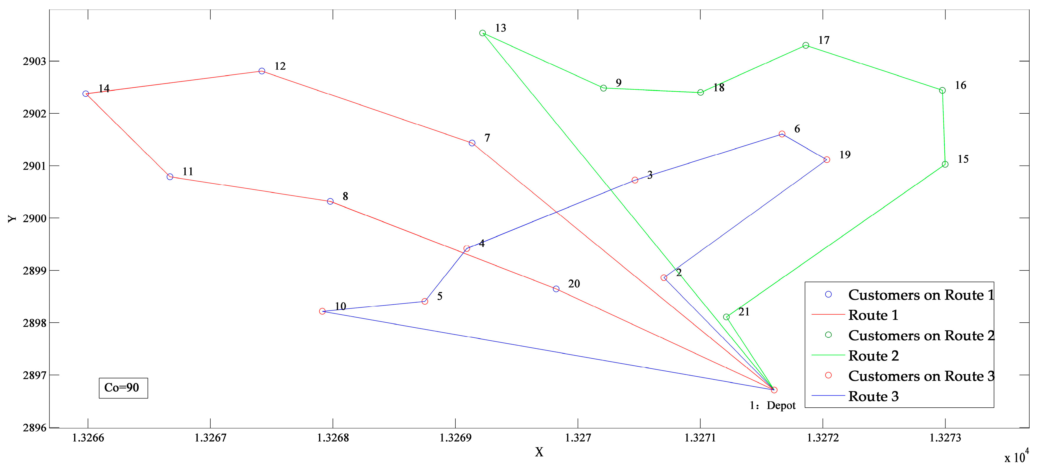
Then, we will verify inference III with the method used to verify inference II. We set to 40, 45, 50, …, 90 for 10 groups of experiments. Each group of data is taken into the model to solve ten times, and then the optimal solution that has optimal fitness value and the optimal distribution path in each group can be selected. The ten sets of data have the same distribution path, which proves that the optimal distribution path does not change. When is set to 40, 70, and 90, the optimal distribution path obtained by solving the model is shown in Figure 10, Figure 11 and Figure 12.
We get the same distribution plan with three sub-paths through Figure 10, Figure 11 and Figure 12. The distribution plan is shown in Table 9.
We analyze the proportion of fixed costs of vehicle , transportation costs , damage costs , refrigeration costs , penalty costs , shortage costs and carbon emission costs in the total cost of distribution C. The cost proportion analysis when is set to 40, 70, and 90 is shown in Table 10, Table 11 and Table 12.
As shown in Table 10, Table 11 and Table 12, the proportion of carbon emission costs () is the highest proportion of all the costs. Thus, we can draw a conclusion that the carbon emission costs determined by carbon tax has a significant impact on the total cost of distribution when . Path optimization is based on the minimum total cost, and carbon emission cost is the highest proportion in total cost. When the carbon tax is increased to the critical value, the path optimization reaches the limit. At this time, the optimal path and carbon footprint no longer changes. This result verifies the correctness of inference III.
From inference II and inference III, we know the carbon emissions will not change with the different carbon tax when the carbon tax is in the range of . As shown in Table 4 and Figure 6, the carbon footprint decreases with the increase of when . It is obvious that inference IV is established.
As the result shows, the cold chain logistics enterprises can reduce the total cost of distribution by optimizing the paths when the carbon tax price gradually increases in the critical range (), and then reduce the cost pressure which is generated from the increase of carbon tax. Objectively, there are also better environmental benefits.
However, when the carbon tax price is out of the critical range (), the effect of carbon tax on path optimization is limited for cold chain distribution network that is already running at the optimal level.
When the increase of carbon tax price led to the increase in the cost of cold chain logistics enterprises beyond their affordability, it is necessary to consider the adoption of technology which is energy-saving and emission-reducing. In short, the change of the carbon tax price in the critical range affects the carbon emission costs, and then affects the total distribution costs of logistics enterprises. The results also provide a reference for government departments to formulate the carbon tax price.
There are two effective means for cold-chain logistics enterprises to reduce the cost pressure brought by the increase of carbon tax; that is, technical measures and path optimization. The use of technical improvement measures requires a large amount of investment; the method of path optimization is to adjust the distribution paths and the order of the service objects to reduce the total cost increase caused by the increase of carbon emission costs, while reducing the carbon emission in the transportation process. Therefore, for the cold chain logistics enterprises, if the carbon tax price is low (), it is entirely possible to use the distribution route optimization method alone to reduce the additional costs associated with the increase in carbon tax, thus making the total distribution costs of enterprises increased slightly and significantly reducing carbon emission. If the carbon tax price is higher (), or the carbon tax is expected to increase significantly in the near future, the cold chain logistics enterprises need to optimize the distribution plan to reduce the distribution cost, and energy-saving and emission-reducing technology, equipment and facilities should be used to achieve the goal of sustainable development of enterprises.
5. Conclusion and Future Works
VRP is a vital problem and a crucial link in reducing the total cost of distribution of cold-chain logistic distribution. VRP and its variants have been studied and solved in many previous works. However, few studies have considered path optimization based on carbon taxes. Besides, the influence of the energy consumption of refrigeration equipment on carbon emissions is often ignored. This paper aims to deal with optimization of VRP with time windows for cold chain logistics based on carbon tax. The carbon emissions in this paper include two aspects: the generation of fuel consumption and the energy consumption of refrigeration equipment. Then, a green and low-carbon cold chain logistics distribution route optimization model with minimum cost is constructed. Taking the lowest cost as the objective function, the total cost of distribution includes the following costs: the fixed costs which generate in distribution process of vehicle, transportation costs, damage costs, refrigeration costs, penalty costs, shortage costs and carbon emission costs.
This paper further proposes the CEGA to solve the model. CEGA simulates the natural evolutionary process of “evolution-degradation” in catastrophism theory, and shows the characteristic of cyclical reciprocation. We combine two kinds of operators, inversion mutation and insertion mutation, in the genetic algorithm to form the combined operator of CEGA. The combination operator is designed to ensure the algorithm can get the optimal solution; that is, the evolution of the algorithm evolves toward the direction of the optimal value of the fitness function. This operator has the feature of keeping the evolution trend of the population to ensure that the periodicity of the CEGA is not a simple reciprocation, but presents a spiral rising characteristic in the general trend.
Low-carbon economy is the new development trend of China’s economy. Government departments in the process of formulating carbon tax should not only consider the socio-economic development, but also take into account the environmental requirements of sustainable development. In the context of full implementation of the carbon emissions trading system in China, logistics companies will face the new problem of how to conduct carbon management in distribution operation decisions. It is especially important to choose the optimal distribution path under different carbon tax. In this paper, the changing trends of carbon emissions and total cost of distribution under different carbon tax are analyzed through an example. The experimental results of this paper provide management suggestions for logistics enterprises to effectively balance economic costs and environmental costs in distribution.
The research of this paper is of great practical significance to the distribution operation of cold chain logistics under the carbon tax mechanism. The results of the study have important reference value for the development of energy-saving and emission-reduction policies in China’s cold chain logistics and transportation industry. The deduction of this paper assumes that only a single enterprise operational decision-making problem is considered, and some conclusions need to be improved in the practical application. It is necessary to do further research on how to deal with cooperation gambling when multiple enterprises face the increase of the carbon tax, and how to consider the uncertainty of demand and the decision-making problem of multiple models based on carbon tax. In addition, some management suggestions are provided in this paper for small- and medium-sized logistics enterprises to effectively control carbon emissions of cold chain logistics and distribution in China’s rural areas. However, there will be a more complex environment in the actual operation of urban distribution, for example, road traffic conditions, multiple distribution centers, multiple types of vehicle and other factors, so it should be further expanded and improved in practical applications. Hence, we offer the following recommendations for future studies. First, real geographical situations can be employed in the distribution path planning. For example, the introduction of road congestion index in the model is better able to reflect the actual feasible solution. Second, additional constraints can be introduced. For example, it is interesting to consider the distribution model under the constraints of multiple distribution centers, multiple types of vehicle and multimodal transport in the future research.
Acknowledgments
The authors would like to thank anonymous referees for their remarkable comments and great support by National Natural Science Foundation of China (No. 71571023).
Author Contributions
Songyi Wang contributed to data analysis and writing the manuscript. Fengming Tao, Yuhe Shi, and Haolin Wen contributed equally to this work designing the empirical analysis, organizing the manuscript and revising analysis.
Conflicts of Interest
The authors declare no conflict of interest.
References
- Wang, X. Changes in CO2 Emissions Induced by Agricultural Inputs in China over 1991–2014. Sustainability 2016, 8, 414–426. [Google Scholar] [CrossRef]
- Piecyk, M.I.; Mckinnon, A.C. Forecasting the carbon footprint of road freight transport in 2020. Int. J. Prod. Econ. 2010, 128, 31–42. [Google Scholar] [CrossRef]
- Jingyuan, Z. Billions of carbon trading market is about to start. People’s Dig. 2016, 22, 46–47. [Google Scholar]
- Dantzig, G.B.; Ramser, J.H. The Truck Dispatching Problem. Manag. Sci. 1959, 6, 80–91. [Google Scholar] [CrossRef]
- Desrochers, M.; Verhoog, T.W. A new heuristic for the fleet size and mix vehicle routing problem. Comput. Oper. Res. 1991, 18, 263–274. [Google Scholar] [CrossRef]
- Solomon, M.M.; Desrosiers, J. Time Window Constrained Routing and Scheduling Problems. Transp. Sci. 1988, 22, 1–13. [Google Scholar] [CrossRef]
- Jabali, O.; Leus, R.; Van Woensel, T.; de Kok, T. Self-imposed time windows in vehicle routing problems. OR Spectr. 2015, 37, 331–352. [Google Scholar] [CrossRef]
- Moghaddam, B.F.; Ruiz, R.; Sadjadi, S.J. Vehicle routing problem with uncertain demands: An advanced particle swarm algorithm. Comput. Ind. Eng. 2012, 62, 306–317. [Google Scholar] [CrossRef]
- Cattaruzza, D.; Absi, N.; Feillet, D. Vehicle routing problems with multiple trips. 4OR 2016, 14, 223–259. [Google Scholar] [CrossRef]
- Laporte, G.; Mercure, H.; Nobert, Y. An exact algorithm for the asymmetrical capacitated vehicle routing problem. Networks 2006, 16, 33–46. [Google Scholar] [CrossRef]
- Righini, G.; Salani, M. New dynamic programming algorithms for the resource constrained elementary shortest path problem. Networks 2005, 51, 155–170. [Google Scholar] [CrossRef]
- Kallehauge, B. Formulations and exact algorithms for the vehicle routing problem with time windows. Comput. Oper. Res. 2008, 35, 2307–2330. [Google Scholar] [CrossRef]
- Pichpibul, T.; Kawtummachai, R. An improved Clarke and Wright savings algorithm for the capacitated vehicle routing problem. ScienceAsia 2012, 38, 307–318. [Google Scholar] [CrossRef]
- Yu, B.; Jin, P.H.; Yang, Z.Z. Two-stage heuristic algorithm for multi-depot vehicle routing problem with time windows. Syst. Eng. Theory Pract. 2012, 32, 1793–1800. [Google Scholar]
- Montané, F.A.T.; Galvão, R.D. A tabu search algorithm for the vehicle routing problem with simultaneous pick-up and delivery service. Comput. Oper. Res. 2009, 33, 595–619. [Google Scholar] [CrossRef]
- Sbihi, A.; Eglese, R.W. Combinatorial optimization and Green Logistics. Ann. Oper. Res. 2010, 175, 159–175. [Google Scholar] [CrossRef]
- Lin, J.; FU, P.; Li, X.; Zhang, J.; Zhu, D. Study on Vehicle Routing Problem and Tabu Search Algorithmunder Low-carbon Environment. Chin. J. Manag. Sci. 2015, 23, 98–106. [Google Scholar]
- Palmer, A. The Development of an Integrated Routing and Carbon Dioxide Emissions Model for Goods Vehicles. Ph.D. Thesis, Cranfield University, Cranfield, UK, 2007. [Google Scholar]
- Maden, W.; Eglese, R.; Black, D. Vehicle Routing and Scheduling with Time-Varying Data: A Case Study. J. Oper. Res. Soc. 2010, 61, 515–522. [Google Scholar] [CrossRef]
- Kuo, Y. Using simulated annealing to minimize fuel consumption for the time-dependent vehicle routing problem. Comput. Ind. Eng. 2010, 59, 157–165. [Google Scholar] [CrossRef]
- Ji, Y.; Yang, H.; Zhou, Y. In Vehicle Routing Problem with Simultaneous Delivery and Pickup for Cold-chain Logistics. In Proceedings of the International Conference on Modeling, Simulation and Applied Mathematics, Phuket, Thailand, 23–24 August 2015. [Google Scholar]
- Yapeng, Z.; Na, L. Research on Elite Selection Based Partheno-genetic Algorithm under Optimized Cold-chain Logistics VRP Model. Math. Pract. Theory 2016, 46, 87–96. [Google Scholar]
- Xiangguo, M.; Tongjuan, L.; Pingzhe, Y.; Rongfen, J. Vehicle Routing Optimization Model of Cold Chain Logistics Based on Stochastic Demand. J. Syst. Simul. 2016, 8, 1824–1832. [Google Scholar]
- Tarantilis, C.D.; Kiranoudis, C.T. Distribution of fresh meat. J. Food Eng. 2002, 51, 85–91. [Google Scholar] [CrossRef]
- Amorim, P.; Parragh, S.N.; Sperandio, F.; Almada-Lobo, B. A rich vehicle routing problem dealing with perishable food: A case study. Top 2014, 22, 489–508. [Google Scholar] [CrossRef]
- Liu, W.Y.; Lin, C.C.; Chiu, C.R.; Tsao, Y.S.; Wang, Q. Minimizing the Carbon Footprint for the Time-Dependent Heterogeneous-Fleet Vehicle Routing Problem with Alternative Paths. Sustainability 2014, 6, 4658–4684. [Google Scholar] [CrossRef]
- Li, X. Development of Cold Chain Logistics in China. In Contemporary Logistics in China: New Horizon and New Blueprint; Wang, L., Lee, S.-J., Chen, P., Jiang, X.-M., Liu, B.-L., Eds.; Springer: Singapore, 2016; pp. 263–288. [Google Scholar]
- Lakshmisha, I.P.; Ravishankar, C.N.; Ninan, G.; Mohan, C.O.; Gopal, T.K. Effect of freezing time on the quality of Indian mackerel (Rastrelliger kanagurta) during frozen storage. J. Food Sci. 2008, 73, 345–353. [Google Scholar] [CrossRef] [PubMed]
- Jinlin, Z.; Jing, X. Review of research on energy conservation and emission reduction of refrigerated vehicle in China. Food Mach. 2013, 29, 236–239. [Google Scholar]
- Xiaoning, W. Vehicles’ Distribution Route Research of Fresh Agricultural Products of Cold Chain Logistics under the Agricultural Super-Docking Mode; East China Jiaotong University: Nanchang, China, 2014. [Google Scholar]
- Duro, J.A. International mobility in carbon dioxide emissions. Energy Policy 2013, 55, 208–216. [Google Scholar] [CrossRef]
- Schafer, A.; Victor, D.G. Global passenger travel: Implications for carbon dioxide emissions. Energy 1999, 24, 657–679. [Google Scholar] [CrossRef]
- Srivastava, S.K. Green supply-chain management: A state-of-the-art literature review. Int. J. Manag. Rev. 2007, 9, 53–80. [Google Scholar] [CrossRef]
- Liguo, Z.; Dong, L.; Dequn, Z. Dynamic Carbon Dioxide Emissions Performance and Regional Disparity of Logistics Industry in China—The Empirical Analysis Based on Provincial Panel Data. Syst. Eng. 2013, 4, 95–102. [Google Scholar]
- Ottmar, R.D. Wildland fire emissions, carbon, and climate: Modeling fuel consumption. For. Ecol. Manag. 2014, 317, 41–50. [Google Scholar] [CrossRef]
- Xiao, Y.; Zhao, Q.; Kaku, I.; Xu, Y. Development of a fuel consumption optimization model for the capacitated vehicle routing problem. Comput. Oper. Res. 2012, 39, 1419–1431. [Google Scholar] [CrossRef]
- Xu, L.; Jia, W.; Ming, H. Application research on improved cyclical virus evdution genetic algorithm. Comput. Integr. Manuf. Syst. 2007, 13, 777–781. [Google Scholar]
- Bermudez, C.; Graglia, P.; Stark, N.; Salto, C.; Alfonso, H. Comparison of Recombination Operators in Panmictic and Cellular GAs to Solve a Vehicle Routing Problem. Iberoam. J. Intel. Artif. 2010, 14, 34–44. [Google Scholar]
- Haifeng, Y.; Xufa, W. Interactive Genetic Algorithm Based on Tournament Selection and Its Application. J. Chin. Comput. Syst. 2009, 30, 1824–1827. [Google Scholar]
- Andreica, A.; Chira, C. Best-order crossover for permutation-based evolutionary algorithms. Appl. Intell. 2015, 42, 751–776. [Google Scholar] [CrossRef]
- Schwartz, Y.; Raslan, R.; Mumovic, D. Implementing multi objective genetic algorithm for life cycle carbon footprint and life cycle cost minimisation: A building refurbishment case study. Energy 2016, 97, 58–68. [Google Scholar] [CrossRef]
- Neng, W.; Meixian, J.; Jiajing, F. A cycle evolutionary genetic algorithm for vehicle routing problem. Machinery 2012, 50, 25–28. [Google Scholar]
- Zhou, L.; Wang, X.; Ni, L.; Lin, Y. Location-Routing Problem with Simultaneous Home Delivery and Customer’s Pickup for City Distribution of Online Shopping Purchases. Sustainability 2016, 8, 828. [Google Scholar] [CrossRef]
- Mcausland, C.; Najjar, N. Carbon Footprint Taxes. Environ. Resour. Econ. 2015, 61, 37–70. [Google Scholar] [CrossRef]
Figure 1.
Description of coding example.
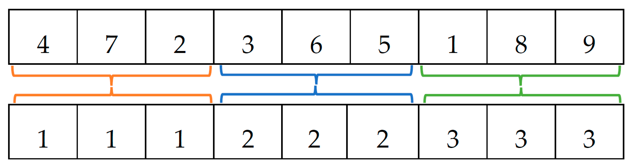
Figure 2.
Examples of cycle crossover procedures.

Figure 3.
Description of inversion mutation example.
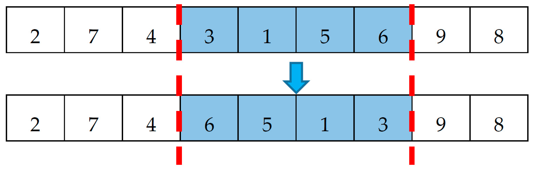
Figure 4.
Description of insertion mutation example.

Figure 5.
Description of interchange mutation example.

Figure 6.
The change of carbon emissions, carbon emission costs and total cost under different carbon tax.
Figure 6.
The change of carbon emissions, carbon emission costs and total cost under different carbon tax.

Figure 7.
The optimal distribution paths when carbon tax is 0.25.

Figure 8.
The optimal distribution paths when carbon tax is 0.5.
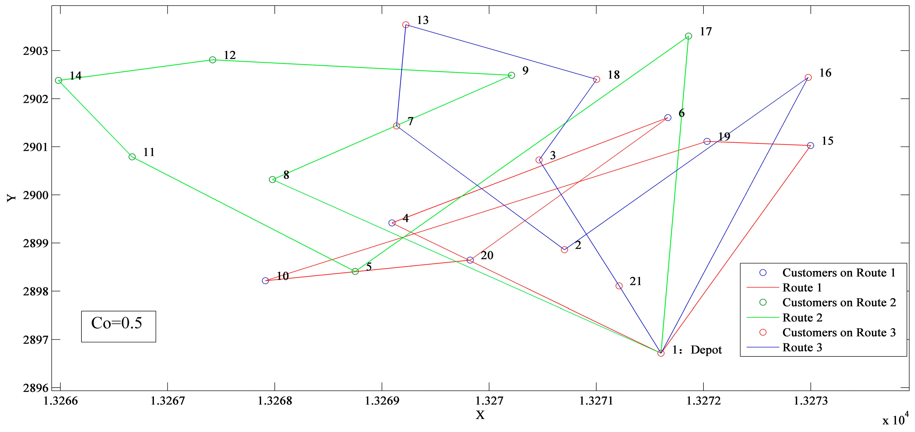
Figure 9.
The optimal distribution paths when carbon tax is 1.0.

Figure 10.
The optimal distribution paths when carbon tax is 40.

Figure 11.
The optimal distribution paths when carbon tax is 70.
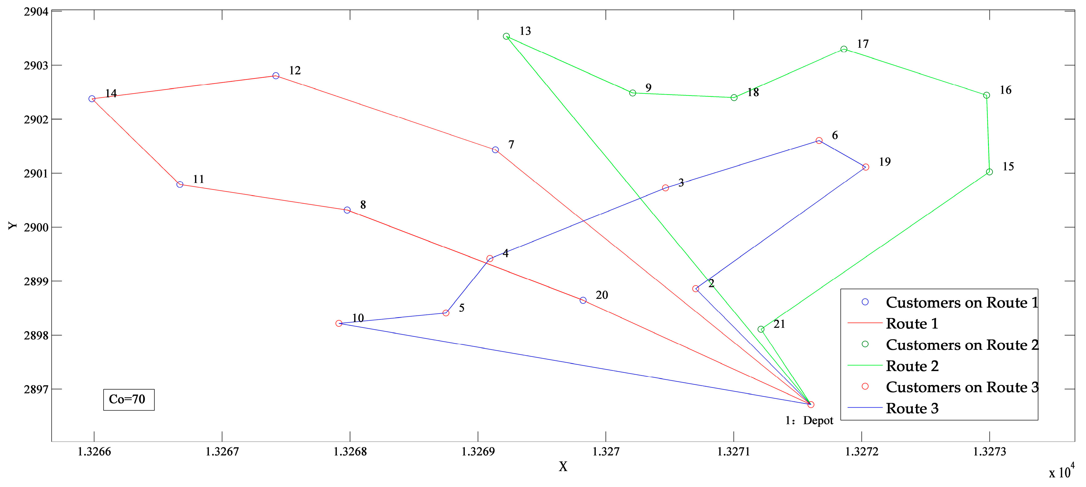
Figure 12.
The optimal distribution paths when carbon tax is 90.


Table 1.
Demand information of customers.
| Number | X Coordinate (km) | Y Coordinate (km) | Demand(t) | The Prescribed Time Window | The Acceptable Time Windows | Service Time (min) |
|---|---|---|---|---|---|---|
| 1 | 13,271.60 | 2896.72 | 0.00 | 5:30–17:00 | 5:00–17:30 | 0 |
| 2 | 13,270.70 | 2898.86 | 1.50 | 6:00–8:00 | 5:30–9:00 | 20 |
| 3 | 13,270.47 | 2900.73 | 0.50 | 7:30–9:00 | 7:00–9:30 | 10 |
| 4 | 13,269.09 | 2899.42 | 1.50 | 6:00–8:00 | 5:30–8:30 | 20 |
| 5 | 13,268.75 | 2898.41 | 1.50 | 6:30–8:20 | 6:00–9:00 | 20 |
| 6 | 13,271.67 | 2901.61 | 2.00 | 6:40–8:30 | 6:10–10:00 | 25 |
| 7 | 13,269.14 | 2901.44 | 2.00 | 7:00–9:00 | 6:30–10:20 | 25 |
| 8 | 13,267.98 | 2900.32 | 1.80 | 7:20–9:00 | 7:00–9:30 | 22 |
| 9 | 13,270.21 | 2902.49 | 1.00 | 7:30–9:00 | 7:00–10:00 | 15 |
| 10 | 13,267.91 | 2898.22 | 1.00 | 7:00–8:30 | 6:40–9:30 | 15 |
| 11 | 13,266.67 | 2900.79 | 1.00 | 7:00–9:00 | 6:30–9:40 | 15 |
| 12 | 13,267.42 | 2902.81 | 1.00 | 7:30–9:30 | 7:00–10:30 | 15 |
| 13 | 13,269.22 | 2903.54 | 0.50 | 7:30–9:00 | 7:00–10:00 | 10 |
| 14 | 13,265.98 | 2902.38 | 0.50 | 7:30–9:30 | 7:00–10:30 | 10 |
| 15 | 13,273.00 | 2901.03 | 1.50 | 7:30–9:00 | 7:00–10:00 | 20 |
| 16 | 13,272.98 | 2902.44 | 2.00 | 6:50–8:30 | 6:20–9:30 | 25 |
| 17 | 13,271.86 | 2903.30 | 1.50 | 7:00–8:40 | 6:40–9:30 | 20 |
| 18 | 13,271.00 | 2902.40 | 1.50 | 7:00–8:40 | 6:40–9:30 | 20 |
| 19 | 13,272.03 | 2901.11 | 0.50 | 7:50–9:00 | 7:00–10:00 | 10 |
| 20 | 13,269.82 | 2898.65 | 2.50 | 6:30–8:30 | 6:00–9:30 | 30 |
| 21 | 13,271.21 | 2898.11 | 1.00 | 7:50–9:00 | 7:00–10:00 | 15 |
Table 2.
Vehicle parameters.
| Parameters | Parameter Values | Parameters | Parameter Values |
|---|---|---|---|
| Outline dimension | 9990 2490 3850 mm | Container size | 7400 2280 2400 mm |
| Total mass | 16,000 kg | Rated load capacity | 9000 kg |
| Engine type | B19 033 | Fuel type | diesel oil |
| No-load fuel consumption in constant speed | 16.5 L/100 km | Integrated fuel consumption | 23.3 L/100 km |
Table 3.
Objective-related parameters.
| Parameter | Value |
|---|---|
| P | 1000 Yuan/t |
| 0.002 | |
| 0.003 | |
| 15 Yuan/h | |
| 20 Yuan/h | |
| 80 Yuan/h | |
| 80 Yuan/h | |
| 100 Yuan/t | |
| 0.377 L/km | |
| 0.165 L/km | |
| 2.630 kg/L | |
| 0.0066/kg·km |
Table 4.
Experimental results for different carbon tax values.
| (Yuan/kg) | Carbon Emission Cost (¥) | Total Cost C (¥) | Carbon Emissions (kg) |
|---|---|---|---|
| 0.00 | 0.00 | 1703.15 | 0.00 |
| 0.25 | 13.54 | 1716.64 | 54.16 |
| 0.50 | 27.10 | 1730.22 | 54.21 |
| 0.75 | 40.98 | 1732.74 | 54.65 |
| 1.00 | 54.56 | 1743.60 | 54.56 |
| 1.50 | 79.19 | 1766.11 | 52.79 |
| 2.00 | 98.98 | 1793.68 | 49.49 |
| 2.50 | 121.49 | 1824.22 | 48.60 |
| 3.00 | 142.05 | 1839.15 | 47.35 |
| 3.50 | 164.22 | 1876.97 | 46.92 |
| 4.00 | 184.74 | 1881.19 | 46.18 |
| 4.50 | 206.18 | 1916.59 | 45.82 |
| 5.00 | 226.20 | 1930.45 | 45.24 |
| 5.50 | 249.81 | 1944.61 | 45.42 |
| 6.00 | 274.07 | 1995.74 | 45.68 |
| 6.50 | 296.33 | 2014.74 | 45.59 |
| 7.00 | 319.70 | 2027.09 | 45.67 |
| 7.50 | 342.27 | 2066.73 | 45.64 |
| 8.00 | 355.33 | 2094.00 | 44.42 |
| 8.50 | 375.58 | 2114.91 | 44.19 |
| 9.00 | 389.98 | 2119.57 | 43.33 |
| 9.50 | 399.51 | 2139.80 | 42.05 |
| 10.00 | 415.78 | 2158.21 | 41.58 |
| 15.00 | 604.62 | 2392.49 | 40.31 |
| 20.00 | 748.88 | 2545.05 | 37.44 |
| 30.00 | 1109.99 | 2924.01 | 37.00 |
| 40.00 | 1437.34 | 3296.93 | 35.93 |
| 50.00 | 1799.58 | 3682.18 | 35.99 |
| 60.00 | 2120.29 | 4037.27 | 35.34 |
| 70.00 | 2471.22 | 4346.58 | 35.30 |
| 80.00 | 2858.46 | 4739.24 | 35.73 |
| 90.00 | 3235.60 | 5171.27 | 35.95 |
Table 5.
The optimal distribution paths when carbon tax is 0.1, 0.5, and 1.0.
| Route Number | Distribution Service Order |
|---|---|
| 1 | 1-4-6-20-10-19-15-1 |
| 2 | 1-17-5-11-14-12-9-8-1 |
| 3 | 1-16-2-7-13-18-3-21-1 |
Table 6.
The proportion of the cost when carbon tax is 0.25.
| Sub-Cost | Amount of Money (¥) | Proportion (%) |
|---|---|---|
| C | 1716.64 | 100.00 |
| 600.00 | 34.95 | |
| 232.95 | 13.57 | |
| 216.84 | 12.63 | |
| 391.72 | 22.82 | |
| 261.60 | 15.24 | |
| 0.00 | 0.00 | |
| 13.54 | 0.79 |
Table 7.
The proportion of the cost when carbon tax is 0.5.
| Sub-Cost | Amount of Money (¥) | Proportion (%) |
|---|---|---|
| C | 1730.22 | 100.00 |
| 600.00 | 34.68 | |
| 237.98 | 13.75 | |
| 215.62 | 12.43 | |
| 390.46 | 22.57 | |
| 259.06 | 14.97 | |
| 0.00 | 0.00 | |
| 54.21 | 3.13 |
Table 8.
The proportion of the cost when carbon tax is 1.0.
| Sub-Cost | Amount of Money (¥) | Proportion (%) |
|---|---|---|
| C | 1743.60 | 100.00 |
| 600.00 | 34.41 | |
| 242.83 | 13.93 | |
| 217.83 | 12.50 | |
| 387.50 | 22.22 | |
| 240.89 | 13.82 | |
| 0.00 | 0.00 | |
| 54.55 | 3.13 |
Table 9.
The optimal distribution paths when carbon tax is 40, 70, and 90.
| Route Number | Distribution Service Order |
|---|---|
| 1 | 1-7-12-14-11-8-20-1 |
| 2 | 1-13-9-18-17-16-15-21-1 |
| 3 | 1-2-19-6-3-4-5-10-1 |
Table 10.
The proportion of the cost when carbon tax is 40.
| Sub-Cost | Amount of Money (¥) | Proportion (%) |
|---|---|---|
| C | 3296.93 | 100.00 |
| 600.00 | 18.20 | |
| 154.75 | 4.70 | |
| 193.26 | 5.86 | |
| 290.75 | 8.82 | |
| 620.83 | 18.83 | |
| 0.00 | 0.00 | |
| 1437.34 | 43.60 |
Table 11.
The proportion of the cost when carbon tax is 70.
| Sub-Cost | Amount of Money (¥) | Proportion (%) |
|---|---|---|
| C | 4346.58 | 100.00 |
| 600.00 | 13.80 | |
| 151.55 | 3.49 | |
| 199.63 | 4.59 | |
| 332.55 | 7.65 | |
| 591.63 | 13.61 | |
| 0.00 | 0.00 | |
| 2471.22 | 56.85 |
Table 12.
The proportion of the cost when carbon tax is 90.
| Sub-Cost | Amount of Money (¥) | Proportion (%) |
|---|---|---|
| C | 5171.27 | 100.00 |
| 600.00 | 11.60 | |
| 154.62 | 3.00 | |
| 194.60 | 3.76 | |
| 292.65 | 5.66 | |
| 643.81 | 12.45 | |
| 50.00 | 0.97 | |
| 3235.60 | 62.59 |
© 2017 by the authors. Licensee MDPI, Basel, Switzerland. This article is an open access article distributed under the terms and conditions of the Creative Commons Attribution (CC BY) license (http://creativecommons.org/licenses/by/4.0/).
Share and Cite
MDPI and ACS Style
Wang, S.; Tao, F.; Shi, Y.; Wen, H. Optimization of Vehicle Routing Problem with Time Windows for Cold Chain Logistics Based on Carbon Tax. Sustainability 2017, 9, 694. https://doi.org/10.3390/su9050694
AMA Style
Wang S, Tao F, Shi Y, Wen H. Optimization of Vehicle Routing Problem with Time Windows for Cold Chain Logistics Based on Carbon Tax. Sustainability. 2017; 9(5):694. https://doi.org/10.3390/su9050694
Chicago/Turabian StyleWang, Songyi, Fengming Tao, Yuhe Shi, and Haolin Wen. 2017. "Optimization of Vehicle Routing Problem with Time Windows for Cold Chain Logistics Based on Carbon Tax" Sustainability 9, no. 5: 694. https://doi.org/10.3390/su9050694
Note that from the first issue of 2016, this journal uses article numbers instead of page numbers. See further details here.