Income Driven Patterns of the Urban Environment

Abstract

This study investigates the land surface temperature (LST) distribution from thermal infrared data for analyzing the characteristics of surface coverage using the Vegetation–Impervious–Soil (VIS) approach. A set of ten images, obtained from Landsat-5 Thematic Mapper, between 2001 and 2010, were used to study the urban environmental conditions of 47 neighborhoods of Porto Alegre city, Brazil. Porto Alegre has had the smallest population growth rate of all 27 state capitals in the last two decades in Brazil, with an increase of 11.55% in inhabitants from 1.263 million in 1991 to 1.409 million in 2010. We applied the environmental Kuznets curve (EKC) theory in order to test the influence of the economically-related scenario on the spatial nature of social-environmental arrangement of the city at neighborhood scale. Our results suggest that the economically-related scenario exerts a non-negligible influence on the physically driven characteristics of the urban environmental conditions as predicted by EKC theory. The linear inverse correlation R² between household income (HI) and LST is 0.36 and has shown to be comparable to all other studied variables. Future research may investigate the relation between other economically-related indicators to specific land surface characteristics.

1. Introduction

The powerful transformation initiated by the economic development in the 19th century is leading civilization to a continuous and rising population migration from rural to urban areas. At the same time, excessive local demands on environmental systems, due to urban growth demand, have become global in scope [1]. Urban areas exist because living in concentrated spaces brings about economic and political advantages [2] in view of the fact that this creates interdependency among people due to the supply and demand for products of physical and spatial perspective [3]. The agglomeration in space, through social and functional organizations, generates constructive densification, which, in turn, makes it possible for people to access more rapidly the activities in a shorter time and distance [4]. Nevertheless, the high constructive and population density, allied with the diversity of activities, can cause the urban areas to enter a degenerative trend, because, while they generate an agglomeration economy, maximizing urban equipment and infrastructure, they equally generate anti-economies [5], like holdups, soaring localization costs and alterations to the urban microclimate in terms of higher temperature. Competition in soil occupation processes mainly due to urbanization and industrialization has been demonstrated to be in disagreement with sustainable development concepts. Nowadays, although there are a number of diverse definitions of urban sustainability, the core value of urban sustainability always lies in the balance of environmental, economic and social development [6,7,8].

In highly urbanized areas, vegetation and impervious surface are two key urban components [9] and combined they are important indicators of environmental quality [10]. Usually, Impervious Surface Areas (ISA) are considered as the complement of vegetation coverage fraction [11].

Cities use construction materials such as concrete and asphalt, which do not allow water to penetrate into the soil, leading to most of the incident shortwave radiation being absorbed and transformed into sensible heat [12]. Thus, under certain imbalanced conditions among percent vegetation coverage, impervious surface types and soil in the urban environment, with a large expanse of non-evaporating impervious materials, there is a consequent increase in sensible heat flux at the expense of latent heat flux [13]. As a result, surface and atmospheric modifications caused by urbanization generally lead to a modified thermal climate, which is warmer than the surrounding non-urbanized areas [14]. This phenomenon, which modulates the air temperature of the lowest layers in the urban atmosphere, is called an Urban Heat Island (UHI). The knowledge about UHI is very important in earth sciences for urban climatology, global environmental change and management practices. UHIs are mainly due to a high percentage of non-reflective, water-resistant surfaces coverage and a low percentage of vegetated and moisture trapping surfaces [15] and are a particular public policy concern during the summer time due to their association with increases in energy, air pollution, and heat stress-related human health. Due to this phenomenon, the distribution of LST has a close relation to the spatial configuration of land cover characteristics in the urban environment [16]. Under these conditions, it is quite conceivable that presence of urban green spaces, moisture trapping surfaces, within other physical characteristics of urban design are always beneficial to mitigating UHI.

In surface areas characterized by fully or fractionally vegetated cover, thermal processes related to direct sunlight interception can significantly influence the surrounding measurements of LST. Furthermore, urban green spaces and trees have been recognized as an important component of urban landscapes [7,8]. Several benefits can be associated with green spaces in the urban environment caused by their capacity for cooling the air [17] and reducing the available surfaces for successively radiating energy reflectance [18]. The evapotranspiration process generated by trees and vegetation in cities can cool the air by using the surrounding urban environment heat from the air to evaporate water [19]. A study from Crompton [20] concluded that a quality forest or green space has a positive economic ripple effect on nearby properties, because urban reforestation in quantity, size and appropriate form makes the cities comfortable and more livable.

In some countries, recent planning and research on the thermal characteristics related to its economic growth have been gaining interest. Studies have shown that urban trees increase the value of residential properties and also make neighborhoods aesthetically more appealing and add to the value of property, regardless of the tree species [21]. The main assumption is that planting trees in cities has high costs and demands planning from policymakers and population in a way that lot size and tree presence reflect, to some extent, the market forces determined by the welfare of the citizens and their preferences [7].

In the 1980s, initial studies relating environmental quality indicators to income were based on the concept of the environmental Kuznets curve (EKC). The EKC effect is an empirical phenomenon and the main assumption of this concept is that economic growth through time is necessary in order for environmental quality to be maintained. This is an essential part of the sustainable development argument [22].

Most of the EKC studies limited the theory to principally problems related to air pollutant concentrations [22]. Recent evidence on the effective mitigation of CO₂ emissions per capita, and cheaper energy use intensity after 2005 [23], has reinforced it in highly developed economies in the world, such as Australia, France, Germany, United Kingdom and United States. Nevertheless, a more recent study from Zhu and Zhang [7] has observed that urban forests were highly related to income for cities with a population over 100,000 in the United States. A detailed study of Escobedo et al. [24] in the city of Santiago, Chile also found that socioeconomic strata were related to different tree cover densities. In Brazil, preliminary analysis from Gusso et al. [25] has shown that high LST averages at neighborhood scale were better spatially linked to those ones with lower sustainability conditions than vegetation index alone. In Australia, the Urban Climates Research (UCR) of the Cooperative Research Centre for Low Carbon Living (CRC-LCL), has been conducting several scale analyses of the urban environment conditions to UHI understanding, urban microclimate analysis, mitigation of carbon emissions and anthropogenic heat generation.

Considering this research issue, a literature review has indicated that thermal remote sensing data obtained from satellites, with adequate temporal and spatial resolution data distribution can improve the understanding of the main surface physical properties in the urban ecosystem conditions [26,27,28,29,30,31].

Currently, the NASA Landsat Data Collection (NLDC) provides historical Landsat data products with medium spatial resolution of 30 m, with a geometric quality of the images that allows the imagery composition for time series analysis and guarantee improved pixel geolocation. Historically, Landsat data have been widely used for urban development and UHI studies, mainly due to its long-term record provided with almost 40 years of data archive [32,33,34] and freely available for research. Landsat data series has an adequate spatial scale for detecting changes over many urban environmental conditions that allows long-term studies of regional and global land cover change [33]. In this context, the launch of the LDCM (Landsat Data Continuity Mission) on 11 February 2013 can also be used for continued urban environment research and management by providing reliable spatial information.

In this study, we demonstrate the influence of socio-economic development on local microclimate conditions in the urban environmental scenario. We go further showing that LST can be used as an integrative indicator of general urban environmental conditions on several levels of social organization in Porto Alegre city in Brazil. Within this approach, we also applied the EKC theory in order to test the influence of the economically-related scenario on the spatial nature of social-environmental arrangement of the city, at neighborhood scale.

2. Materials and Methods

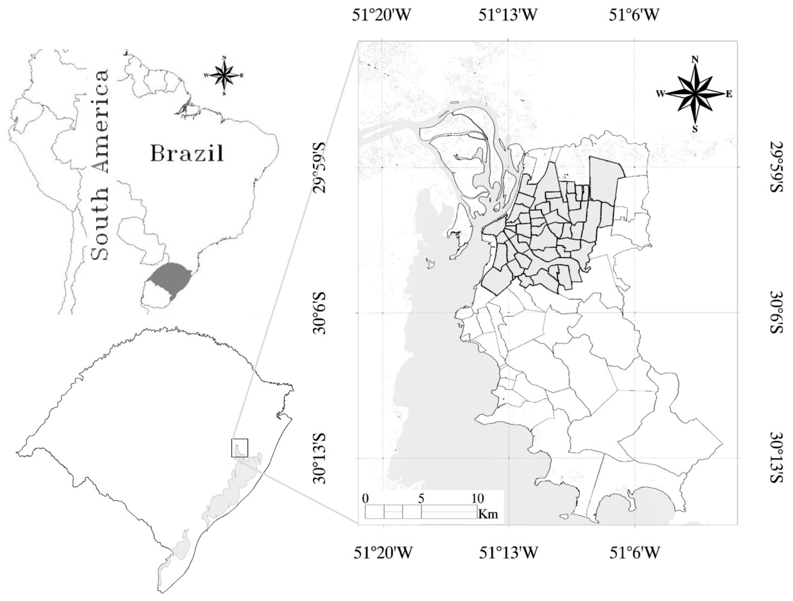
2.1. Study Area

The study area is the city of Porto Alegre, which is the capital of Rio Grande do Sul State (RS) and was founded on 26 March 1772. The city is the capital of the most southern state in Brazil and it is located at latitude of 30°01′59′′ South and longitude of 51°13′48′′ West. Porto Alegre is well suited to this study because it has passed through a period of slow growth in the last two decades, with an increase of 11.55% in inhabitants from 1.263 million in 1991 to 1.409 million in 2010. This represents the smallest population growth rate of all 27 capitals in Brazil and far lower than the overall average growth rate of capitals with 43.75% and also from overall Brazilian average of 29.92% [35].

After the 1930s, the ten most common trees species in the city are deciduous and cover almost 85% of public areas [36]. However, regarding most of urbanized neighborhoods of the city, several years under a prevailing weak economic growth and increasing public debts of RS state, associated with a lack of maintenance of urban green spaces, have led to diverse conditions of its urban environment compared to most of big cities in Brazil. Since then, recovery actions for public urban green spaces have been implemented after 2000 by the new Urban Forestry Plan (UFP) of Porto Alegre City [36]. Most common tree species are: extremosa (Lagerstroemia indica)—India, with an incidence of 19.50%; ligustro (Ligustrum japonicum)—endemic, with 18.64%; jacarandá (Jacarandá mimosifolia)—endemic, with 10.75%; cinamomo (Melia azedarach)—China, with 5.7%; perna-de-moça (Brachychyton populneum)—endemic with 4.12%; ipê roxo (Tabebuia heptaphylla)—endemic with 3.10%; mimo-de-vênus (Hibiscus rosa-sinenis)—endemic, with 2.84%; ipê amarelo (Tabebuia chrysotricha)—endemic, with 2.56%; and tipuana (Tipuana tipu)—Argentina, with 1.67% [36].

The region predominantly experiences a subtropical mid-latitude climate (Cfb) with four well-defined seasons [37]. The mean annual temperature is 19.5 °C, with monthly averages varying between 12 °C and 26 °C. The monthly mean precipitation is 114 mm and the yearly-accumulated average precipitation is 1373 mm with no dry period. Figure 1 shows the study area. The city is completely covered with a Landsat scene (Path 221 and Row 081). The neighborhood scale elevation average of the study area is 39 m above the sea level with a standard deviation (SD) of 14 m. The maximum average altitude is 103 m and minimum is 7 m. The study area comprises 47 densely populated neighborhoods surrounding the downtown, covering a total area of 9077 ha.

2.2. Satellite Imagery and Data Set

Absolute LST measures are commonly used in physiological studies because they is related to vegetation canopy [38]. Multi-temporal imagery analysis is essential for UHI studies [39]. LST obtained from satellite imagery is, strictly speaking, a measure of the “skin temperature” or surface radiometric energy (kinetic) emitted from the land surface and is related to the thermal infrared (TIR) radiation from surface rather than air temperature [40].

The Landsat data series satellites have collected several years of data in the thermal spectral band and have been used in several studies for UHI [41]. However, the challenge in urban environmental LST estimation is the numerous factors that need to be quantified in order to assess accurate LST retrieval from thermal satellite data. Those factors include sensor radiometric calibration [42,43], atmospheric correction [44,45,46], simplified atmosphere approaches [39] but mainly surface emissivity correction [47] and changing physically driven dynamics of land coverage through time [32,48]. Due to radiometric and atmospheric conditions only ten images were selected. The generated image product is composed of cloud-free images covering the 47 neighborhoods studied.

The information levels and data sources included in this study are the following:

• Landsat-5 TM imagery from 2000 to 2010, Path and Row 221-081 [49];
• Shuttle Radar Topography Mission (SRTM) data [50], version 3, product GL1, were used to analyze the relationship between elevation and distribution of other variables studied on a 30-meter spatial resolution [49];
• Monthly rainfall data obtained from the Database for Meteorological Research [51], which covers the period from October to December, were used to identify possible drought periods in the warmest season;
• Soil types map in a 1:5,000,000 scale [52];
• Census data of Neighborhoods limits and urban sectors [35];
• Census data of Population by neighborhoods in 2010 [35];
• Climatological norm of accumulated rainfall from October to December [51,53];
• Census data of Household Incomes (Brazilian salary units) at neighborhood scale, from 2000 and 2010 [35];
• Digital geospatial reference from National Aeronautics and Space Administration-Global Land Survey [49].

2.3. Calibration and Data Generation

2.3.1. Reflectance Data Generation

Timely analysis based on remote sensing data, such as the Landsat series, requires accurate input parameters from meta data, ground based meteorological measurements and look up tables based on surface-related parameters [33,54,55]. Full absolute image correction includes atmospheric and sensor-related parameters and then the derivation of physical units, such as reflectance [18]. Planetary reflectance (or apparent) is limited by atmospheric characteristics. To compare imaged targets at different times and locations and even to compare targets imaged by different sensors required transforming the images to reflectance of the surface, since this is a target property, and which can be compared for checking differences and surface modeling parameters. In this way, a complete rescaling calibration and correction of digital numbers (DN) was performed by NASA for the conversion of DN into Top-of-Atmosphere (TOA) reflectance data according to a time-dependent calibration look-up tables (LUT), generated from the lifetime gain model equations for all bands. This methodology substitutes the previous National Landsat Archive Production System (NLAPS) based on internal instrument calibration procedure [55].

In order to overcome future difficulties related to complex vicarious calibration processes and methodologies it is very important to develop an independent technical source for satellite instrument calibration to ensure confidence in the accuracy, interoperability, and quality of satellite observations reducing analysis uncertainties [56]. Independent algorithms allow continuous monitoring and provide transparency to the methodology. Transparency is needed not only to permit other investigators to scrutinize the quality of the data, but also so they can pursue alternative research inquiries because parameters, literature and adjacent supporting methodologies are not always available and published [57]. Thus, the calibration and validation have been primary to the measurements obtained from satellites and surface parameters determinations through satellite images [54]. With this purpose in mind, the radiometric calibration has the purpose of ensuring the update of the quality of data generated by a remotely located sensor and ensuring the possibility of converting the data recorded by the sensors to physical quantities that can be correlated to geophysical parameters [58].

Regarding the calibration of reflectance channels, for the accurate transformation of radiance into TOA and then into surface reflectance data, the images were also atmospherically corrected according to [44], because atmospheric conditions are spatially and temporally significant [55].

First, DN were converted into radiance and next to reflectance, according to the calibration parameters of [55] and LST [42]. After conversion to at-satellite radiance, each image was converted to at-satellite reflectance (assuming a uniform Lambertian surface under cloudless conditions) according to the general mathematical function for reflectance calculation shown in Equation (1). Radiometric calibration coefficients and parameters were obtained from [55].

The TOA calculation can be described by applying the simple radiance–reflectance conversion for each band of LANDSAT-5 TM according to Equation (1).

$$\rho =\frac{\pi \times L_{\lambda }\times d^2}{ESU{N}_{\lambda }\times cos{\theta }_z}$$

(1)

where L_λ is the spectral radiance at the sensor in each band (W·m⁻²·sr⁻¹·μm⁻¹); d is the distance between the Earth and the Sun in astronomic units (UA); ESUN_λ is the average solar exoatmospheric irradiance (W·m⁻²·μm⁻¹); and θ_z is the solar zenith angle (degrees).

The atmosphere correction process is applied by substituting for the term L obtained during the DN conversion to radiance by the factor (L_sat − L_p)/T_z when correcting TOA to canopy-surface reflectance in the Equation (1), according to Equations (2)–(4). The atmosphere correction process is based on the Dark-Object Subtraction (DOS) concept which depends on the wavelength of visible bands and assumes near-zero percent reflectance of specific features [18]. The DOS approach is related to a weighted displacement effect to each band on a per-pixel-basis, according to the processes described in [44,59]. By using this approach, the data necessary to perform atmospheric correction in the visible bands 1–5 from Landsat 5 TM can be obtained from the image itself [47] by restricting the atmospheric influence, as the radiation transfer from the Earth’s surface to on-orbit sensors. As an additional control for radiometric quality and a reduction in the amount of atmosphere effects, Landsat-5 TM imagery was submitted to a threshold criterion for the image processing protocol from [48], whereby no image was used when the amount of atmospheric contamination effects exceeded 70 DN in the blue band (452–518 μm), of Landsat-5 TM.

$${\rho }_{surf}=\frac{\pi \times (L_{sat}-L_p)\times d^2}{ESU{N}_{\lambda }\times cos{\theta }_z\times T_z}$$

(2)

$$L_p=L_{min}-L_{1\%}$$

(3)

$$L_{1\%}=\frac{0.01\times cos{\theta }_z\times T_z\times ESU{N}_{\lambda }}{\pi \times d^2}$$

(4)

where ρ_surf is the canopy-surface reflectance; L_sat is the radiance at the sensor in each band (W·m⁻²·sr⁻¹·μm⁻¹); L_p upwelling atmospheric spectral radiance scattered (W·m⁻²·sr⁻¹·μm⁻¹); T_z atmospheric transmittance along the path from the sun to the ground surface; L_min total radiance of first-order scattering component if DN < 0.01% (W·m⁻²·sr⁻¹·μm⁻¹); and L_1% is the radiance of Dark Object assuming reflectance = 0.01 (W·m⁻²·sr⁻¹·μm⁻¹).

2.3.2. Classification of Surface Cover Types

Once the surface reflectance by correcting TOA reflectance was calculated, we applied an empirical reflectance-based method. The VIS approach from Ridd [9] conceptualizes an urban environment in terms of three primary physical components: vegetation (V), impervious surfaces (I), and soil (S) coverage [11]. The modified VIS model considered the spectral signature of pixel covering urban areas as a linear combination of those three components.

Impervious surface areas (ISA) are surfaces where water cannot infiltrate and are primarily associated with transportation (streets, highways, parking lots and sidewalks) and building rooftops. ISA extractions based on an image classification is a complex task and is often underestimated due to the heterogeneity of urban landscapes due its complexity [60]. ISA calculation is based mainly on identifying and categorizing the spectral profile of highly reflective surfaces such as pavements, rooftops and buildings, non-vegetated or even sparsely vegetated areas. At pixel and sub-pixel level, impervious surfaces may be mixed with other land cover types, such as trees, grasses, and soils [60].

The non-blue band versions of Enhanced Vegetation Index (EVI-2) can be computed and then can be used on the LST-emissivity dependence calculation. The adequate correction of atmospheric effects is very important because it will allow correct EVI-2 values to be generated, which will also be used for the classification of surface coverage types. EVI-2 is a two-band version of EVI that has been developed for sensors without a blue band [61]. Reflectance values from bands 3 and 4 were used to generate the EVI-2 data according to Equation (2) from Jiang et al. [61]. EVI-2 retains sensitivity and the same as EVI for high leaf area index (LAI) canopies, but does not rely on the usually poor-quality blue band [62]. In this way, EVI-2 calculation (Equation (5)) can be used as an acceptable substitute of EVI over atmospherically corrected pixels [61].

Soil classification was obtained by considering those pixels that were not classified either urban neither densely vegetated areas.

$$EVI2=2.5\times \frac{NIR-Red}{NIR+2.4\times Red+1}$$

(5)

where NIR, Red, Green and Blue represent the obtained reflectance in the near-infrared, red, green and blue bands of Landsat-5 TM at a given pixel, respectively; and EVI-2 is the no-blue band Enhanced Vegetation Index (EVI).

2.3.3. Thermal Data Generation

Regarding the thermal analysis from Landsat 5 TM band 6, after converting DN into absolute radiance values, LST is computed from at-satellite brightness temperatures (i.e., blackbody temperature) using pre-launch calibration constants [42,55] and under the assumption of emissivity factor equal to unity [63]. Under this assumption (ε_NB = 1), the conversion of the detected thermal radiation into brightness temperature is given in Equation (10), [55], which is a special case of Plank’s radiation law. In order for LST to become representative of realistic surface conditions at this point, the LST still needs to be corrected to more realistic values of non-unity surface emissivity [42,64] by means a robust technique of emissivity dependent LST retrieval. Surface emissivity is controlled by factors, such as water content, chemical composition, structure and roughness [65].

This formulation does not result on directly corrections to atmospheric effects (absorption and emissions along the path) because of the difficulty with estimating water vapor content from thermal detection in the mono-window band 6 [63]. In the thermal channel, atmospherically corrected surface conditions can be obtained using an indirect estimation of physical characteristics from atmospherically corrected reflectance of surface in the visible bands, according to the previously mentioned Equation (2).

Emissivity calculation for non-black body surface with the narrow band adjustment (NB) for Landsat data series depends on the empirical equation of Soil Adjusted Vegetation Index (SAVI) from [66]. Parameters SAVI and LAI are obtained from previously atmospherically corrected band 1 and 2. The value for L in SAVI formulation (Equation (7)) can be derived from analysis of multiple images where vegetation does not change, but surface soil moisture does. According to [66] optimal value of L = 0.5 (light soil < L = 0.5 < dark soil) must be used to account for first-order soil background variations. Afterwards, SAVI (Equation (7)) was used for calculation of the LAI which parameters were empirically obtained from Equation (8) according to [67]. Finally, the adjusted LST (hereafter LST) is obtained by correcting the radiating surface temperature to the surface emissivity (ε), at pixel scale as given by Equation (9), which is the ratio of the thermal energy radiated by the surface to the thermal energy radiated by a blackbody at the same temperature [67,68,69], as follows:

$$LST=\frac{K2}{ln\left(\frac{{\epsilon }_{NB}\times K1}{L}+1\right)}$$

(6)

where LST is the emissivity-corrected surface temperature (K); K1 is the calibration constant 1 (607.76 W·m⁻²·sr⁻¹·μm⁻¹); K2 is the calibration constant 2 (1260.56 W·m⁻²·sr⁻¹·μm⁻¹); L is the blackbody radiance of the thermal band 6 (W·m⁻²·sr⁻¹·μm⁻¹); and ε_NB is the emissivity factor, which depends on the type of surface coverage conditions; when LAI > 3.0, ε_NB = 0.98 because the increased water content in vegetation actually increases emissivity capacity.

$$SAVI=\frac{\left(1+L\right)\times \left(NIR-Red\right)}{\left(L+NIR+Red\right)}$$

(7)

$$LAI=-\frac{ln\left(\frac{0.69-SAVI}{0.59}\right)}{0.91}$$

(8)

$${\epsilon }_{NB}=0.97+0.0033\times LAI$$

(9)

where L is the constant parameter in SAVI with value 0.5; SAVI is the Soil Adjusted Vegetation Index; and LAI is the Leaf Area Index empirically adjusted.

2.4. LST and Biophysical Descriptors

Although the presence of trees in urban ecosystems is primarily conceptualized in terms of the aesthetic, environmental, and wildlife habitat functions [70], it is well known that shade trees and even small plants for land cover, help cool the urban environment [71].

In the natural environment, dry, bare and low-density soils, for example, have been linked to higher LST as a result of the relatively low thermal inertia [72]. These thermal properties vary with the type of soil and moisture content [72]. On the other hand, in the urban environment, non-evaporative and impervious surface areas not only play an important role in UHI formation [13] but also in heat generated by anthropogenic sources, such as traffic and industries [31]. This is because the emissivity of soils or sparsely vegetated areas is a function of soil moisture conditions and soil density [31,48,73]. The physical fundamentals for such a relationship rely on the fact that for any surface material, certain internal properties, such as heat capacity, thermal conductivity and inertia, play important roles in governing the temperature of a body at equilibrium with its surroundings [74].

In the summer season, generally 10%–30% of the sun’s energy reaches the area below a tree, with most of it being absorbed by leaves and used for photosynthesis and some being reflected back into the atmosphere [71]. Even so, thermal responses for vegetation can also vary highly as a function of the biophysical properties of the vegetation itself [16,75]. The inverse relationship between thermal characteristics of surface and vegetation indices has been extensively documented in the literature [31,73]. This concept is based on the assumption that vegetation coverage mitigates high LST occurrence values [48]. Given this and considering that temperature is closely related to physiological activities of vegetation cover, LST can be a useful measure of the physiological activity of the top canopy leaves when leaf cover is sufficiently high such that they are not affected by background temperature from soil [38]. However, vegetation index measurements are subject to seasonal variations, which may influence the results on UHI studies, and thus, such vegetation index measurements alone may not serve as a good indicator for urban development [31].

Regarding the seasonal effects and fluctuation of vegetation cover conditions, it is well known that in drought-free years, well-developed vegetation reflects only a small portion of incident solar radiation in the visible band of the spectrum because of chlorophyll absorption properties and other plant pigments that absorb sunlight [32]. In the NIR, plants reflect much more because of a scattering effect caused by the internal structure and water content of leaves [76].

Furthermore, the percentage of impervious surfaces coverage under green vegetated areas can also change with very small variations on vegetation index values. Based on studies from Zhu and Zhang [7], which accounted for tree number distributed in the urban environment, we aggregated the public and private trees among the city environment into one single variable, which is representative of the amount of vegetation.

2.5. TSDS Approach

The study of LST is closely related to the distribution of LULC characteristics. Models that describe LULC can provide a link between LST and physical spatial distribution in a way that absolute values of LST are not key fundamental variables for the understanding of its distribution is. This is because LST is highly variable through time and does not allow the comparison of absolute values in a simplified conceptual approach.

Detailed studies from [31], conducted in the metropolitan area of Minnesota (US), found that the vegetation index–LST relationship is more suitable for the analysis of UHI during summer and early autumn. In this way, for a better understanding of the physical descriptors of heating effects over the urban environment, as a representative of their development through time, we only compared the summer season imagery from late December to February, in a way to detect the most pronounced LST values associated with surface coverage. In this paper, the absolute temperature fluctuations through time have thus not been evaluated. Instead, the focus is on the evaluation of the trend of LST-emissivity dependent in neighborhoods related and its distribution.

A previous analysis of the LST distribution was done by applying the Thermal Spatial Distribution Signature (TSDS) procedure. The TSDS procedure [25,48] using TIR data obtained from Landsat-5 TM was applied as a criterion for multi-temporal imagery combination of data, which is based on the relation between the thermal characteristics of surface and coverage and consists of the standard deviation (SD) analysis of LST to compare images by means similarity characteristics. Thus, to evaluate the most precise combination data for multi-temporal analysis, the key question is: what are the time windows and their extension for performing an adequate imagery combination in order to perform a reliable LULC diagnosis [48]?

According to Gusso et al. [48], when studying a histogram of LST distribution through time, it is expected that the highly urbanized or sparsely vegetated areas are unable to cool the surrounding sensible heat by evapotranspiration, as they typically do. Such fractional vegetation and soil cover conditions leads to a spread of the LST range by increasing statistical indicators in terms of the variance of distribution towards higher LST values [48].

3. Results

3.1. Data Retrieval

After choosing a selection of image groups by means of the TSDS approach, we can compare overall data retrieved between neighborhoods for surface coverage types and LST (

Table 1. Selected Landsat-5 TM imagery for monitoring the studied area.

	Acquisition	θZ-90	LST (K)			EVI-2			Surface Cover Types (%)
	Date	(deg)	Min.	Max.	Average	Min.	Max.	Average	Vegetation	ISA	Soil
01	1 January 2001	55.6	293.95	310.59	304.47	0.0	0.91	0.22	28.70	65.48	5.51
02	2 February 2001	51.6	291.53	303.12	297.42	0.0	0.74	0.23	30.28	64.97	4.44
03	20 January 2002	53.5	294.01	303.95	299.56	0.0	0.68	0.21	22.48	72.12	5.16
04	11 February 2004	50.1	289.90	304.37	298.07	0.0	0.73	0.21	23.55	70.29	5.66
05	12 January 2005	57.0	287.55	313.59	305.20	0.0	0.68	0.19	17.31	74.33	7.89
06	2 January 2007	59.5	294.91	307.64	301.69	0.0	0.88	0.22	25.01	68.49	5.99
07	3 February 2007	53.9	298.38	314.94	307.77	0.0	0.74	0.22	24.33	69.37	5.80
08	6 February 2008	53.5	290.36	305.19	298.27	0.0	0.71	0.21	21.86	72.71	4.70
09	7 January 2009	56.6	288.97	303.12	296.55	0.0	0.72	0.22	23.03	71.05	5.23
10	11 February 2010	51.8	287.73	300.60	294.67	0.0	0.76	0.22	22.58	74.67	2.28

,

Table 2. Summary of retrieved averages obtained from the selected Landsat-5 TM.

Imagery	θZ-90		Radiometric Estimators				Surface Cover Types
Date	(deg)	SD	LST (K)	SD	EVI-2	SD	%Vegetation	SD	%ISA	SD	%Soil	SD
2001 to 2010	54.31	2.87	300.38	4.26	0.215	0.01	23.91	3.61	70.35	3.34	5.27	1.41

Note: SD: Standard Deviation.

and

Table 3. General descriptive statistics retrieved for each neighborhood.

Neighborhood	Radiometric Estimators				Surface Cover Types (VIS)						Terrain-Socio-Economic
Name	LST (K)	SD	EVI-2 (Dim.)	SD	%Veg.	SD	%ISA	SD	%Soil	SD	HI (Salaries)	Alt. (m)	Pop. D. (inh/ha)
Auxiliadora	300.1	0.70	0.17	0.06	4.6	3.6	89.7	3.3	7.0	1.4	9.8	36.8	114.3
Azenha	301.0	0.76	0.16	0.07	6.4	3.6	91.3	3.3	2.9	1.4	5.6	16.5	8.0
Bela Vista	298.7	0.56	0.22	0.08	17.6	3.6	77.9	3.3	6.3	1.4	17.6	67.7	118.8
Boa Vista	299.8	0.86	0.26	0.12	35.9	3.6	60.4	3.3	5.6	1.4	12.0	46.0	5.5
Bom Fim	300.5	0.49	0.14	0.05	1.2	3.6	96.1	3.3	2.3	1.4	7.7	24.9	24.2
Bom Jesus	300.7	0.73	0.20	0.07	11.6	3.6	88.0	3.3	1.9	1.4	2.7	79.3	146.8
Cel. A. Borges	300.1	1.29	0.27	0.10	40.6	3.6	58.9	3.3	2.5	1.4	2.6	99.2	60.0
Centro	299.6	1.07	0.12	0.07	5.0	3.6	90.3	3.3	4.4	1.4	6.5	24.8	181.2
Chácara das P.	300.3	0.51	0.21	0.06	9.7	3.6	90.1	3.3	1.7	1.4	12.7	60.6	61.7
Cidade Baixa	300.8	0.63	0.14	0.06	3.6	3.6	94.8	3.3	3.1	1.4	5.9	12.3	21.8
Cristo Red.	301.4	0.63	0.17	0.06	6.6	3.6	92.5	3.3	1.8	1.4	5.7	33.4	109.9
Farroupilha	298.6	1.25	0.29	0.13	48.9	3.6	44.6	3.3	8.9	1.4	8.9	18.4	15.8
Floresta	301.7	0.57	0.11	0.05	0.6	3.6	97.1	3.3	2.1	1.4	6.0	12.7	91.0
Glória	300.3	0.84	0.23	0.09	23.7	3.6	72.1	3.3	6.6	1.4	4.7	50.9	81.9
Higienópolis	299.9	0.61	0.20	0.07	10.5	3.6	83.3	3.3	6.7	1.4	10.7	45.5	99.7
Independência	300.1	1.00	0.16	0.08	6.0	3.6	90.4	3.3	3.8	1.4	9.9	43.6	231.8
Jard. Botânico	299.5	1.55	0.25	0.12	32.2	3.6	64.0	3.3	5.6	1.4	7.5	27.6	59.5
Jard. Carvalho	299.8	1.59	0.26	0.11	32.9	3.6	63.6	3.3	4.4	1.4	3.6	64.6	80.6
Jard. do Salso	299.6	1.32	0.27	0.11	39.6	3.6	56.6	3.3	5.7	1.4	6.6	39.6	46.8
Jard. Floresta	300.9	0.64	0.23	0.09	22.8	3.6	77.2	3.3	2.7	1.4	3.4	17.4	46.8
Jard. Itú Sab.	300.1	1.41	0.26	0.11	32.1	3.6	66.5	3.3	2.9	1.4	6.4	55.4	46.5
Jard. Lindoia	300.8	0.60	0.19	0.07	10.3	3.6	86.7	3.3	5.3	1.4	9.6	20.8	99.4
Jard. São Ped.	300.5	0.76	0.24	0.12	36.6	3.6	62.7	3.3	2.6	1.4	5.6	12.3	5.3
Medianeira	300.6	0.98	0.20	0.08	11.4	3.6	85.9	3.3	4.5	1.4	5.4	40.3	63.2
Menino Deus	300.3	0.75	0.18	0.07	8.6	3.6	88.4	3.3	3.8	1.4	8.7	14.9	14.2
Moinhos de V.	299.2	0.65	0.21	0.09	18.1	3.6	76.0	3.3	8.5	1.4	16.1	41.5	79.6
Mont Serrat	299.5	0.80	0.20	0.06	8.1	3.6	88.5	3.3	4.6	1.4	12.5	63.6	133.1
Navegantes	301.3	0.93	0.11	0.06	1.4	3.6	96.1	3.3	3.4	1.4	3.5	7.4	20.6
Partenon	300.5	1.26	0.22	0.10	22.8	3.6	75.7	3.3	2.9	1.4	4.1	45.9	79.0
Passo da Areia	301.1	1.10	0.20	0.11	16.0	3.6	82.1	3.3	2.7	1.4	5.7	24.6	85.3
Passo das P.	300.4	1.39	0.26	0.12	35.1	3.6	63.0	3.3	4.1	1.4	3.4	41.5	113.6
Petrópolis	299.4	0.99	0.21	0.09	16.0	3.6	77.3	3.3	8.4	1.4	10.7	54.1	110.3
Rio Branco	299.6	1.00	0.18	0.07	9.0	3.6	87.0	3.3	5.2	1.4	12.0	42.2	119.5
Santa Cecilia	300.6	0.60	0.18	0.09	15.0	3.6	81.4	3.3	5.0	1.4	7.6	17.1	80.5
Santa Tereza	299.5	1.43	0.26	0.11	34.9	3.6	61.0	3.3	5.7	1.4	3.5	59.7	114.0
Santana	300.7	0.52	0.15	0.06	3.2	3.6	93.1	3.3	4.8	1.4	7.1	14.7	161.7
Santo Antônio	300.2	0.79	0.23	0.10	24.8	3.6	72.2	3.3	4.4	1.4	5.2	55.0	99.1
São Geraldo	301.7	0.73	0.12	0.05	1.4	3.6	95.4	3.3	4.7	1.4	4.3	9.8	56.9
São Joao	301.0	1.57	0.23	0.14	33.1	3.6	60.4	3.3	7.4	1.4	6.6	8.7	29.4
São Jose	300.3	1.44	0.22	0.07	18.9	3.6	80.1	3.3	2.6	1.4	2.2	102.7	140.2
São Sebastião	301.0	0.63	0.19	0.07	8.4	3.6	89.4	3.3	3.8	1.4	4.2	22.1	138.2
Sarandi	300.8	1.57	0.22	0.12	23.9	3.6	73.6	3.3	3.4	1.4	2.6	12.0	94.5
Sta. M. Goretti	301.1	0.87	0.15	0.06	6.7	3.6	91.9	3.3	2.6	1.4	4.4	9.0	4.2
Três Figueiras	299.5	0.93	0.26	0.10	32.4	3.6	62.7	3.3	6.6	1.4	17.7	73.2	3.0
Vila Ipiranga	300.7	1.09	0.23	0.10	25.3	3.6	77.5	3.3	2.3	1.4	5.9	48.0	92.0
Vila Jardim	300.7	0.61	0.21	0.06	12.7	3.6	87.9	3.3	1.6	1.4	4.0	89.4	87.4
Vila João P.	301.4	0.48	0.19	0.06	6.3	3.6	94.3	3.3	1.3	1.4	3.2	39.5	132.6

). By adequately combining all imagery data, the major patterns of LST distribution could be identified. The overall average of the LST, from all 10 images selected, was 300.36 K (27.21 °C) with a standard deviation of 1.34 K. This low value of standard deviation compared to the mean is also indicative of a robust technique.

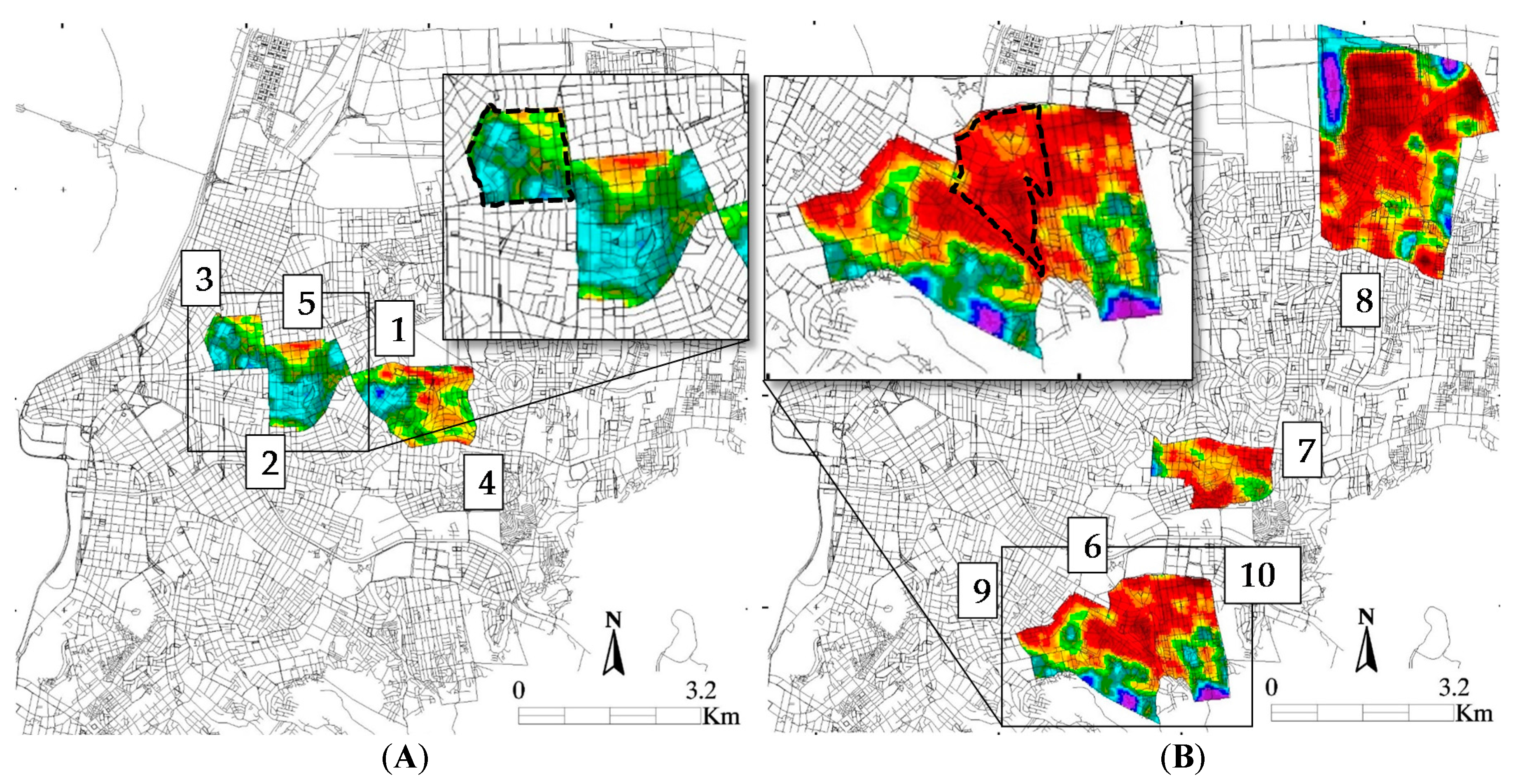
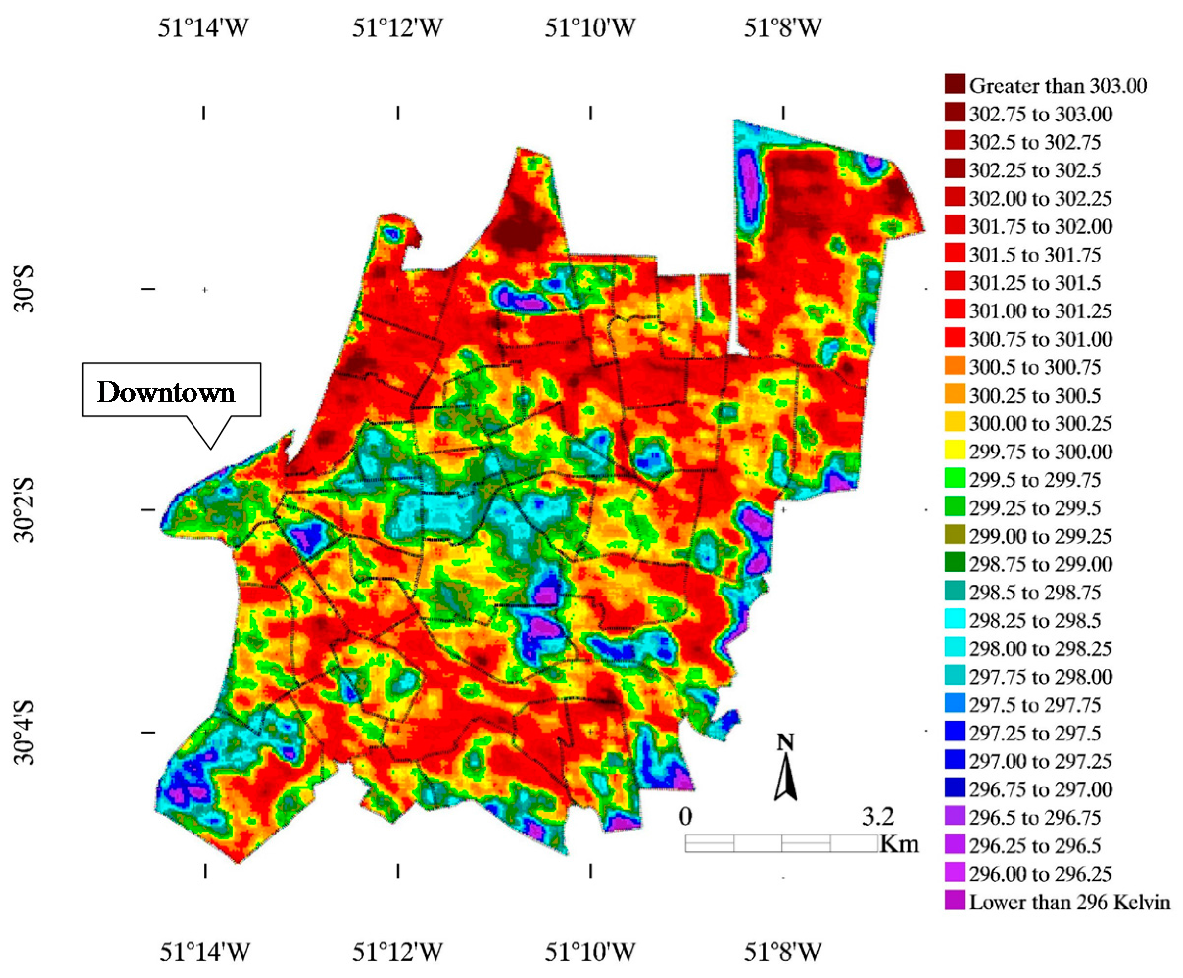
3.2. Spatially Distributed Patterns of UHI

On the pixel scale, differences of 10.71 K, were found in the LST distribution. Maximum absolute LST with 305.80 K (32.65 °C) was found at São João and minimum of 295.09 K (21.94 °C) was found at Jardim Botânico. On the neighborhood scale, differences of 2.83 K were found between neighborhoods averages. Maximum LST average of neighborhood with 301.67 K (28.52 °C) was found at São Geraldo which is characterized by low vegetated areas coverage with high density of impervious coverage. The minimum LST average of 298.65 K (25.50 °C) was found at Farroupilha which is characterized by highly vegetated coverage area and where ISA do not prevail.

Regarding the analysis of LST dependence to EVI-2, we have found that the main pattern is a clear core distribution of lower LST values located at the center of the study area (dark blue and green) which is surrounded by higher LST values (dark red and orange). The lower LST configuration is associated with high maintenance residential area and the higher LST values are representative of main arterial avenues and streets of the city. Most of the higher LST averages were observed in the northern neighborhoods, also called as the 4th district, especially São Geraldo (301.67 K), Floresta (301.66 K), Cristo Redentor (301.37 K) and Vila João Pessoa (301.35 K). There are two main factors that stand out for the higher LST in Porto Alegre, as also observed by [25]: (1) physically, they are related to the installation of surface train facilities in April 1985 that goes out to the north, spreading to the adjacent neighborhoods, with a further enhancement of impervious surfaces and avenues; and (2) economically, there is a concentration of most industrial plants, corporate services and companies located in these regions. Furthermore, UHI mitigation strategies involving vegetation tend to be more expensive per unit area than strategies involving high-albedo surfaces [77], such as rooftops and industrial facilities. These two factors are interrelated to the increase of pollution, population decline and imbalance in land use between impervious surfaces and vegetation coverage.

Regarding the lower LST cluster at the middle of the study area, we found that they are mostly covering residential areas. Lower LST values were observed in the center-southern neighborhoods (orange and dark red), especially the Farroupilha (298.65 K), Bela Vista (298.68 K), Moinhos de Vento (299.17 K) and Petrópolis (299.40 K). There are two main factors that stand out for the lower LST in Porto Alegre: (1) physically, they are distributed as a concentration of residential ones; and (2) economically, there is a concentration of parks and malls located within these neighborhoods.

Figure 2 shows the LST averages covering the urban area of Porto Alegre city obtained from all selected images in the study area.

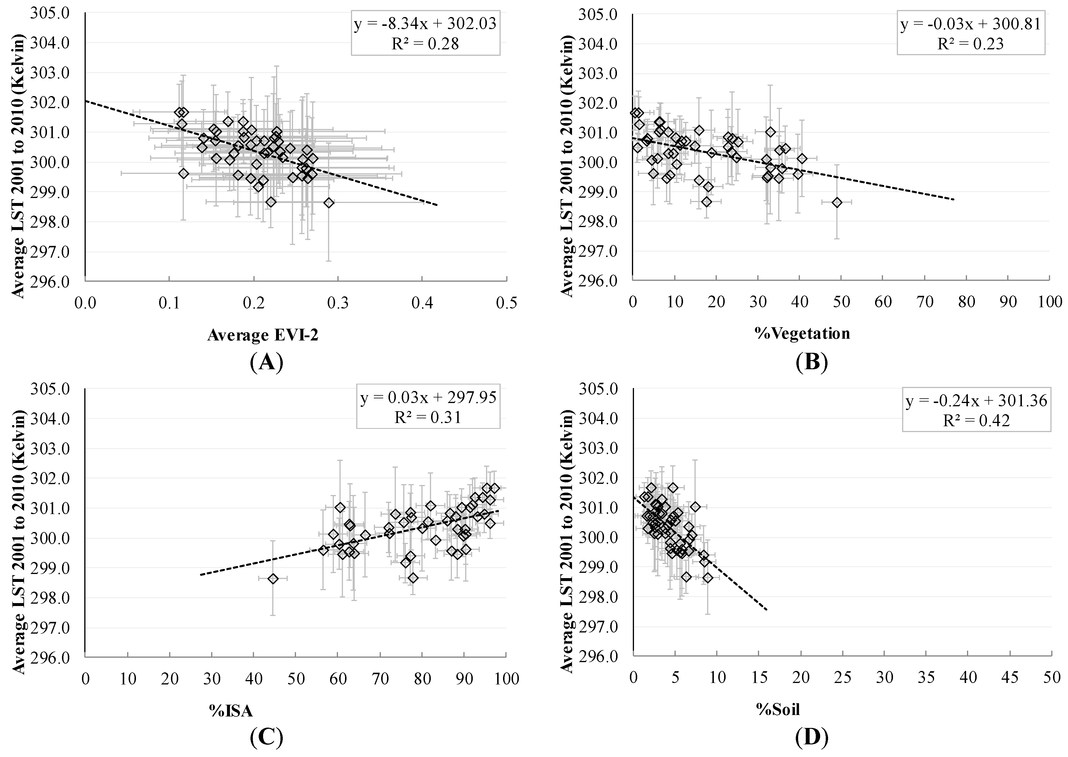
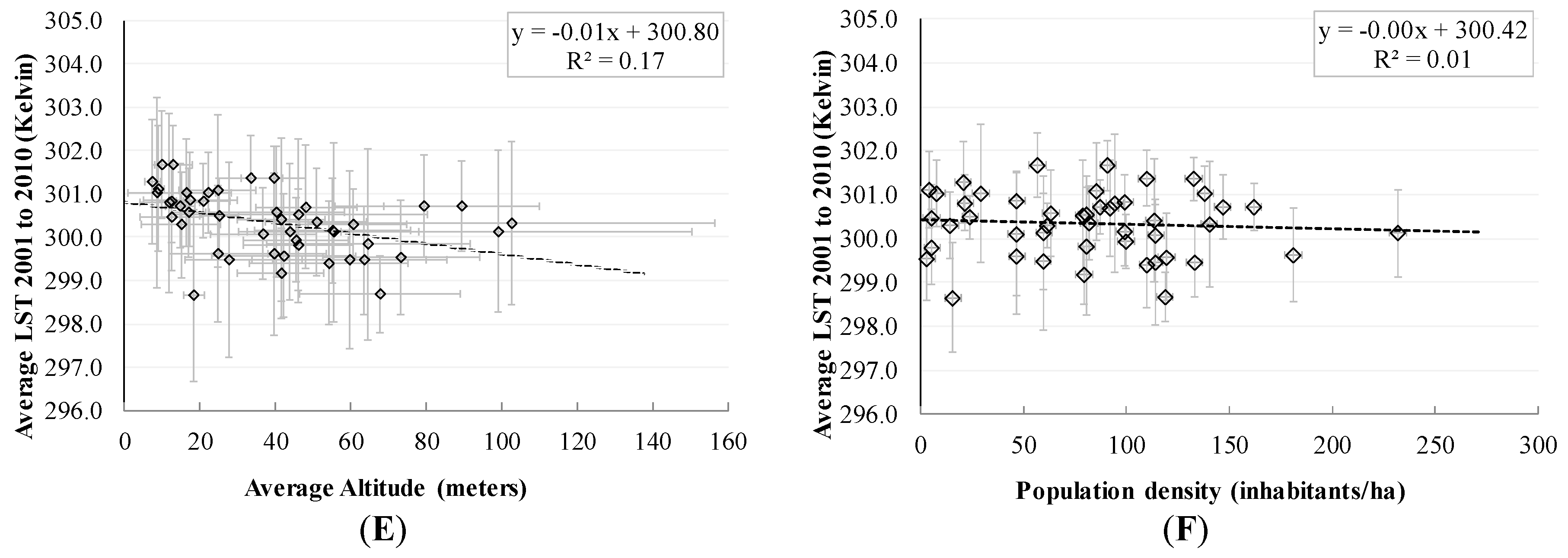
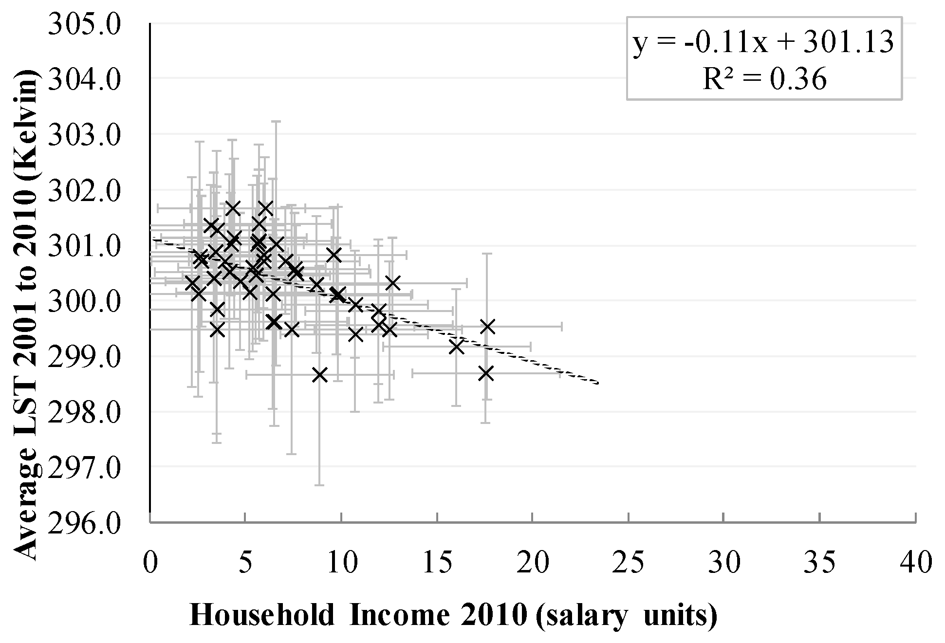
3.3. Analysis of Surface Physical Descriptors

Each neighborhood in Porto Alegre city has different characteristics caused by the patterns of the prevailing urban development over the past decades. Different combinations of VIS play an important role in the LST distribution. Thus, an analysis of the connection of VIS surface cover types with LST distribution was performed. For simplicity, correlations were established by using a negative first order polynomial function as described by the mathematical equation y = −β × x + γ.

Our results show that the simple analysis of %Vegetation indicates a poor correlation to LST averages (R² = 0.23) as expected, and %ISA (R² = 0.31). However, %Soil coverage plays a major role possibly because it is indirectly related to vegetation coverage and the soil moisture associated to soil background in green areas. This result is probably linked to the fact that the empirical model used in this study for VIS surface type classification considered sparsely vegetation coverage and non-impervious surfaces as the same set of soil surface coverage type. Even so, although %Soil (or sparsely vegetation presence) does show a better correlation to LST averages distribution, it does not express any spatiality regarding its values as the UHI patterns recognized in Figure 2.

In general, we have found poor correlation of physical variables VIS, Altitude or Population density to LST as shown in Figure 3. Although studies from Yuan and Bauer [31] identified that LST is better correlated to percent of impervious surfaces than vegetation index, the physical conditions and properties of the vegetation types and surrounding urban environment also have important influence on determination of LST distribution [78] as well for soil surface area. As it can be seen in Figure 3B,C results show that %ISA increases due to urbanization and subsequently leads to %Vegetation decrease according [79]. Even so, it is possible to find some dense canopy trees in areas of almost completely impervious surfaces at surface level. Regarding low correlation of %Vegetation and Vegetation density (EVI-2) to LST averages, the main reason probably is linked to the fact that vegetation density by itself does not represent value on the real estate configuration. In this way, higher surface vegetation coverage (%Vegetation) are not necessarily representative of green areas and structured and humanized urban green spaces.

Based on the emissivity dependence of LST to EVI-2, we applied the EKC concept to test the correlation between the welfare due to the social-environmental arrangement of the citizens (Household Income) and LST distribution at neighborhood scale. On the analysis of LST distribution associated to HI, a better correlation was found by using a negative first order polynomial function as described by the mathematical equation y = −β × x + γ in Figure 4.

On the neighborhood scale, results show a linear inverse correlation (R² = 0.36) between HI and LST averages. Physically, it is expected that there is a superior threshold to those higher LST averages as function of surface coverage conditions. Table 3 shows descriptive statistics obtained from socio-economic and satellite data.

3.4. Urban Development Modelling

The different urban microclimates show alterations that stem from the loss of vegetation cover combined with soil imperviousness that come from the density and constructive compactness which are directly related to the rising socioeconomic development of these areas. Thus, to test the relation observed between the environmental variable to the economical one, we analyzed the spatially distributed dependence of LST averages to HI by means of a mathematically combination of the ratio (as Household Income/LST average) because they are inversely related. We obtained a rank which is adequately associated to the spatial distribution of UHI clusters in the city of Porto Alegre.

Results in Figure 5A,B indicate that the ratio between HI and LST averages increases the rank when LST is lower and HI is high, which can be considered as an indicator of better urban development conditions. The ratio decreases when LST averages are higher and HI is lower which, in the same way, can be considered as representative of not well developed urban areas. The Top 5 ranked neighborhoods are: (1) Três Figueiras; (2) Bela Vista; (3) Moinhos de Vento; (4) Chácara das Pedras; and (5) Mont Serrat. The Bottom 5 ranked neighborhoods are: (6) Vila João Pessoa; (7) Bom Jesus; (8) Sarandi; (9) Cel. Aparício Borges; and (10) São José.

4. Discussion

These ranked results, which are essentially the same as HI alone, suggest that there is an economical influence on the historical formation of neighborhoods. The main lower ranked cluster and its adjacent areas are characterized by a particular and historical behavior in the urban environment development. Vila João Pessoa (between São José and Cel. Aparício Borges) is the first suburban neighborhood, formed around 1940, and developed along with the same sub-standard conditions through decades without adequate planning [80]. Most of Vila João Pessoa population still live in a society with no fixed job, and survive on the collection of waste (industrial waste, plastic bottles). In 2010, the average income of residents of Vila João Pessoa was 3.23 salary units. The average for the entire Porto Alegre city, with the 83 neighborhoods, was 5.3 salary units ranging between 1.84 to 18.24 salary units [80]. On 4 January 2010, the value of 1 salary unit (monthly payment) was on average equivalent to US$296.5 [81].

Considering the main higher ranked cluster and its adjacent areas, Moinhos de Vento (Windmills) is characterized by a particular historical behavior in the urban environment development. It was formed right after arrival of the Açorianos (migrants from the Açores Islands region, of Portugal), in 1772. The windmills were brought by the Açorianos and had its apogee during the wheat cultivation period. Even so, after 1835, the cultivation in the region was abandoned. Neighborhood development was boosted in 1893 with tram line installation, implemented for public transportation by urban municipality company “Carris”. Another driving factor for the Moinhos de Vento development was the construction of hydraulic facilities in the hills of the area, in 1904, which led to the opening of several nearby streets. In the southern border of the neighborhood area the German Hospital took place in 1927, which in 1942 was renamed Hospital Moinhos de Vento [80]. Still today, it is one of the best and most modern city facilities. In 2010, the average income of residents of Moinhos de Vento was 16.05 salary units. Nowadays, it exhibits high-standard conditions and with adequate urban planning maintaining higher well-infrastructured conditions of green spaces and residential areas. Such results suggest that the economic resulting geolocation is a function of a veiled and underlying sectoring of city areas which, by its turn, promotes an environmentally unsustainable configuration of sub-urban areas but which is not directly related to imperviousness, vegetation coverage, soil exposure or lot size.

The spatial distribution of the districts and villages in the territory of the city, in general, tend to reflect the distribution of the various social segments. Peripheral squatter settlements, either legal or clandestine, devoid of infrastructure, in different parts of the city, can present higher environmental temperature rates due to denser soil occupation. Ultimately, such macro-scale results observed from satellite imagery indicate that there is need for environmental maintenance in the lower ranked neighborhoods. These results indicate that not only the prevailing physically driven conditions in the urban environment but also the social environmental arrangement associated mainly to infrastructure and aesthetically configuration of neighborhoods, is exerting a non-negligible influence on LST distribution. This also suggests that reduced quality of public administration and management policies thorough years has been contributing to the precarious environmental situation of some neighborhoods, which in its turn can also lead to the strengthening of low educational status of individuals [80].

5. Conclusions

Results suggest that the economically-related scenario exerts a non-negligible influence on the physically driven characteristics of the urban environmental conditions as predicted by EKC theory.

Different combinations of VIS surface cover types play an important role on the LST distribution. However, the characteristics of the urban environmental conditions that can be detected by thermal remote sensing are linked to the aspects that are associated with different levels of social organization in the urban contexts that cannot be objectively measured, including public administration efficiency, welfare, education or even sustainable urban environment concept which also depends on social and economic standards. In this way, the investigation on the association between the HI and LST averages at neighborhood scale has been demonstrated to be straightforward for the understanding of the development process that leads to UHI. This study will also be available as documentation of the existing findings on UHI in Porto Alegre city and thus can help further research.

Finally, we also conclude that even at the neighborhood scale, there are variables regarding social organization, public management and city design that should be considered when studying urban development and environmental conditions [82]. Future research may investigate the relationship between other economically-related variables to specific land surface characteristics.

References

1. Brown, L. World on the Edge; W.W. Norton & Company: New York, NY, USA, 2011; p. 325. [Google Scholar]
2. Marshall, A. Princípios de Economia; Nova Cultural: São Paulo, Brazil, 1996. [Google Scholar]
3. Krafta, R. Modelling intra-urban configurational development. Environ. Plan. B 1994, 21, 67–82. [Google Scholar] [CrossRef]
4. Ioppolo, G.; Heijungs, R.; Cucurachi, S.; Salomone, R.; Kleijn, R. Urban Metabolism: Many Open Questions for Future. In Pathways to Environmental Sustainability: Methodologies and Experiences; Salomone, R., Saija, G., Eds.; Springer: Dordrecht, The Netherlands, 2014; pp. 23–32. [Google Scholar]
5. Harvey, D. The Urbanization of Capital; John Hopkins Press: Baltimore, Maryland, 1985. [Google Scholar]
6. Shen, L.; Kyllo, J.M.; Guo, X. An Integrated Model Based on a Hierarchical Indices System for Monitoring and Evaluating Urban Sustainability. Sustainability 2013, 5, 524–559. [Google Scholar] [CrossRef]
7. Zhu, P.; Zhang, Y. Demand for urban forests in United States cities. Landsc. Urban Plan. 2008, 84, 293–300. [Google Scholar] [CrossRef]
8. Zhu, P.; Zhang, Y. Demand for urban forests and economic welfare: Evidence from the Southeastern U.S. cities. J. Agric. Appl. Econ. 2006, 38, 279–285. [Google Scholar] [CrossRef]
9. Ridd, M.K. Exploring a V–I–S (Vegetation–Impervious Surface–Soil) model for urban ecosystem analysis through remote sensing: Comparative anatomy for cities. Int. J. Remote Sens. 1995, 16, 2165–2185. [Google Scholar] [CrossRef]
10. Arnold, C.L.; Gibbons, C.J. Impervious Surface Coverage: The emergence environmental of a key environmental indicator. J. Am. Plan. Assoc. 1996, 62, 243–258. [Google Scholar] [CrossRef]
11. Zhang, C.; Cooper, H.; Selch, D.; Meng, X.; Qiu, F.; Myint, S.W.; Roberts, C.; Xie, Z. Mapping urban land cover types using object-based multiple endmember spectral mixture analysis. Remote Sens. Lett. 2014, 5, 521–529. [Google Scholar] [CrossRef]
12. Landsberg, H.E. The Urban Climate; Academic Press: New York, NY, USA, 1981. [Google Scholar]
13. Owen, T.W.; Carlson, T.N.; Gillies, R.R. Remotely sensed surface parameters governing urban climate change. Int. J. Remote Sens. 1998, 19, 1663–1681. [Google Scholar] [CrossRef]
14. Voogt, J.A.; Oke, T.R. Thermal remote sensing of urban climates. Remote Sens. Environ. 2003, 86, 370–384. [Google Scholar] [CrossRef]
15. Rosenzweig, C.; Solecki, W.D.; Parshall, L.; Chopping, M.; Pope, G.; Goldberg, R. Characterizing the urban heat island in current and future climates in New Jersey. Environ. Hazards 2005, 6, 51–62. [Google Scholar] [CrossRef]
16. Hatvani-Kovacs, G.; Belusko, M.; Skinner, N.; Pockett, J.; Boland, J. Heat stress risk and resilience in the urban environment. Sustain. Cities Soc. 2016, 26, 278–288. [Google Scholar] [CrossRef]
17. Bruntland, G. Our Common Future: The World Commission on Environment and Development; Oxford University Press: New York, NY, USA, 1987. [Google Scholar]
18. Schroeder, T.A.; Cohen, W.B.; Song, C.; Canty, M.J.; Yang, Z. Radiometric Correction of Multi-Temporal Landsat Data for Characterization of Early Successional Forest Patterns in Western Oregon. Remote Sens. Environ. 2006, 103, 16–26. [Google Scholar] [CrossRef]
19. Li, J.; Song, C.; Cao, L.; Zhu, F.; Meng, X.; Wu, J. Impacts of Landscape Structure on Surface Urban Heat Islands: A Case Study of Shanghai, China. Remote Sens. Environ. 2011, 115, 3249–3263. [Google Scholar] [CrossRef]
20. Crompton, J.L. Parks and Economic Development; American Planning Association: Chicago, IL, USA, 2001. [Google Scholar]
21. Anderson, L.M.; Cordell, H.K. Influence of Trees on Residential Property Values in Athens, Georgia (U.S.A.): A Survey based on Actual Sales Prices. Landsc. Urban Plan. 1988, 15, 153–164. [Google Scholar] [CrossRef]
22. Stern, D.I. International Society for Ecological Economics—Internet Encyclopaedia of Ecological Economics. The Environmental Kuznets Curve; Department of Economics, Rensselaer Polytechnic Institute: Troy, NY, USA, 2003; p. 18. [Google Scholar]
23. United States Energy Information Administration (EIA). International Data on CO2 Emissions. Available online: http://www.eia.gov/cfapps/ipdbproject/IEDIndex3.cfm?tid=90&pid=44&aid=8 (accessed on 2 July 2016).
24. Escobedo, F.J.; Novak, D.J.; Wagner, J.E.; De la Maza, C.L.; Rodriguez, M.; Crane, D.E.; Hernandéz, J. The socioeconomics and management of Santiago de Chile's public urban forests. Urban For. Urban Green. 2006, 4, 105–114. [Google Scholar] [CrossRef]
25. Gusso, A.; Cafruni, C.; Bordin, F.; Veronez, M.R.; Lenz, L.; Crija, S. Multi-Temporal Patterns of Urban Heat Island as Response to Economic Growth Management. Sustainability 2015, 7, 3129–3145. [Google Scholar] [CrossRef]
26. Jauregui, E. Heat island development in Mexico City. Atmos. Environ. 1997, 31, 3821–3831. [Google Scholar] [CrossRef]
27. Streutker, D.R. Satellite-measured growth of the urban heat island of Houston, Texas. Remote Sens. Environ. 2003, 85, 282–289. [Google Scholar] [CrossRef]
28. Defense Meteorological Satellite Program—U.S. Department of Defense. 2013. Available online: http://go.nature.com/u7b6Os (accessed on 9 July 2015).
29. Hung, T.; Daisuke, U.; Shiro, O.; Yoshifumi, Y. Assessment with satellite data of the urban heat island effects in Asian mega cities. Int. J. Appl. Earth Obs. Geoinform. 2006, 8, 34–48. [Google Scholar]
30. Liu, H.; Weng, Q. An examination of the effect of landscape pattern, land surface temperature, and socioeconomic conditions on WNV dissemination in Chicago. Environ. Monit. Assess. 2009, 159, 143–161. [Google Scholar] [CrossRef] [PubMed]
31. Yuan, F.; Bauer, M.E. Comparison of impervious surface area and normalized difference vegetation index as indicators of surface urban heat island effects in Landsat imagery. Remote Sens. Environ. 2007, 106, 375–386. [Google Scholar] [CrossRef]
32. Gusso, A.; Ducati, J.R. Algorithm for Soybean Classification Using Medium Resolution Satellite Images. Remote Sens. 2012, 4, 3127–3142. [Google Scholar] [CrossRef]
33. Irons, J.R.; Dwyer, J.L.; Barsi, J.A. The Next Landsat Satellite: The Landsat Data Continuity Mission. Remote Sens. Environ. 2012, 122, 11–21. [Google Scholar] [CrossRef]
34. Barsi, J.A.; Schott, J.R.; Hook, S.J.; Raqueno, N.G.; Markham, B.L.; Radocinski, R.G. Landsat-8 Thermal Infrared Sensor (TIRS) Vicarious Radiometric Calibration. Remote Sens. 2014, 6, 11607–11626. [Google Scholar] [CrossRef]
35. Instituto Brasileiro de Geografia e Estatística—System for Automatic Data Retrieval. (IBGE-SIDRA). Available online: http://www.sidra.ibge.gov.br/ (accessed on 12 December 2015).
36. Prefeitura Municipal de Porto Alegre—Plano Diretor de Arborização Urbana (PMPA-PDAU). Available online: http://www2.portoalegre.rs.gov.br/smam/default.php?reg=1&p_secao=8 (accessed on 17 February 2015).
37. Köppen, W. Climatologia: Con un Estúdio de los Climas de la Tierra; Fondo de Cultura Econômica: Tlalpan, Mexico, 1948; p. 466. (In Spanish) [Google Scholar]
38. Sims, D.A.; Rahman, A.F.; Cordova, V.D.; El-Masri, B.Z.; Baldocchi, D.D.; Bolstad, P.V.; Flanagan, L.B.; Goldstein, A.H.; Hollinger, D.Y.; Misson, L.; et al. A New Model of Gross Primary Productivity for North American Ecosystems Based Solely on the Enhanced Vegetation Index and Land Surface Temperature from MODIS. Remote Sens. Environ. 2008, 112, 1633–1646. [Google Scholar] [CrossRef]
39. Ogashawara, I.; Bastos, V.S.B. A Quantitative Approach for Analyzing the Relationship between Urban Heat Islands and Land Cover. Remote Sens. 2012, 4, 3596–3618. [Google Scholar] [CrossRef]
40. Qin, Z.; Karnieli, A.; Berliner, P. A Mono-Window Algorithm for Retrieving Land Surface Temperature from Landsat TM Data and its Application to the Israel-Egypt Border Region. Int. J. Remote Sens. 2001, 22, 3719–3746. [Google Scholar] [CrossRef]
41. Callejas, I.J.A.; Oliveira, A.S.; Santos, F.M.M.; Durante, L.C.; Nogueira, M.C.J.A.; Zeilhofer, P. Relationship between land use/cover and surface temperatures in the urban agglomeration of Cuiabá-Várzea Grande, Central Brazil. J. Appl. Remote Sens. 2011, 5, 1–15. [Google Scholar] [CrossRef]
42. Markham, B.L.; Barker, J.L. Landsat MSS and TM Post-Calibration Dynamic Ranges, Exoatmospheric Reflectances and at-Satellite Temperatures; Landsat Tech. Note 1; Earth Observation Satellite Co.: Lanham, MD, USA, 1986. [Google Scholar]
43. Wukelic, G.E.; Gibbons, D.E.; Martucci, L.M.; Foote, H.P. Radiometric Calibration of Landsat Thematic Mapper Thermal Band. Remote Sens. Environ. 1989, 28, 339–347. [Google Scholar] [CrossRef]
44. Chavez, P.S., Jr. Image-Based Atmospheric Correction—Revisited and Improved. Photogramm. Eng. Remote Sens. 1996, 62, 1025–1036. [Google Scholar]
45. Souza, J.D.; Silva, B.B. Correção atmosférica para temperatura da superfície obtida com imagem TM—Landsat-5. Rev. Bras. Geogr. Fís. 2005, 23, 349–358. [Google Scholar] [CrossRef]
46. Jiménez-Munõz, J.C.; Cristóbal, J.; Sobrino, J.A.; Sòria, G.; Ninyerola, M.; Pons, X. Land Surface Temperature Retrieval from LANDSAT TM 5. IEEE Trans. Geosci. Remote Sens. 2009, 47, 339–349. [Google Scholar] [CrossRef]
47. Sobrino, J.A.; Jiménez-Munõz, J.C.; Paolini, L. Land Surface Temperature Retrieval from LANDSAT TM 5. Remote Sens. Environ. 2004, 90, 434–440. [Google Scholar] [CrossRef]
48. Gusso, A.; Veronez, M.R.; Robinson, F.; Roani, V.; Da Silva, R.C. Evaluating the thermal spatial distribution signature for environmental management and vegetation health monitoring. Int. J. Adv. Remote Sens. GIS 2014, 3, 433–445. [Google Scholar]
49. United States Geological Survey (USGS)—Earth Resources Observation & Science Center (EROS). Available online: http://earthexplorer.usgs.gov/ (accessed on 15 February 2014).
50. Rabus, B.; Eineder, M.; Roth, A.; Bamler, R. The shuttle radar topography mission: A new class of digital elevation models acquired by spaceborne radar. ISPRS J. Photogramm. Remote Sens. 2003, 57, 241–262. [Google Scholar] [CrossRef]
51. Instituto Nacional de Meteorologia (INMET). Available online: http://www.inmet.gov. br/portal/index.php?r=bdmep/bdmep (accessed on 12 February 2015).
52. Instituto Brasileiro de Geografia e Estatística—Soil Classification and Maps. Available online: http://mapas.ibge.gov.br/tematicos/solos (accessed on 15 January 2015).
53. WorldClim—Global Climate Data, Free Climate Data for Ecological Modeling and GIS. Available online: http://www.worldclim.org/tiles.php. (accessed on 1 January 2016).
54. Teillet, P.M.; Fedosejevs, G.; Gauthier, R.P.; O’Neill, N.T.; Thome, K.J.; Biggar, S.F.; Ripley, H.; Meygret, A. A generalized approach to the vicarious calibration of multiple Earth observation sensors using hyperspectral data. Remote Sens. Environ. 2001, 77, 304–327. [Google Scholar] [CrossRef]
55. Chander, G.; Markham, B.L.; Helder, D.L. Summary of Current Radiometric Calibration Coefficients for Landsat MSS, TM, ETM+, and EO-1 ALI Sensors. Remote Sens. Environ. 2009, 113, 893–903. [Google Scholar] [CrossRef]
56. Wu, X.; Goldberg, M. Global space-based inter-calibration system (GSICS): A status report. Atmospheric and Environmental Remote Sensing Data Processing and Utilization III: Readiness for GEOSS. Proc. SPIE 2007, 6684. [Google Scholar] [CrossRef]
57. Hooker, B.; McClain, C.R.; Mannino, A. A Comprehensive Plan for the Long Term Calibration and Validation of Oceanic and Biogeochemical Satellite Data; NASA/SP-2007-214152; National Aeronautics and Space Administration (NASA): Washington, DC, USA, 2007.
58. Ponzoni, F.J.; Pinto, C.T.; Lamparelli, R.A.C.; Junior, J.Z.; Antunes, M.A.H. Calibração de Sensores Orbitais; Oficina de Textos: São Paulo, Brasil, 2015. [Google Scholar]
59. Chavez, P.S. An Improved Dark-Object Subtraction technique for atmospheric scattering correction of multispectral data. Remote Sens. Environ. 1988, 24, 459–479. [Google Scholar] [CrossRef]
60. Lu, D.; Weng, Q. Use of impervious surface in urban land-use classification. Remote Sens. Environ. 2006, 102, 146–160. [Google Scholar] [CrossRef]
61. Jiang, Z.; Huete, A.R.; Didan, K.; Miura, T. Development of a Two-Band Enhanced Vegetation Index without a Blue Band. Remote Sens. Environ. 2008, 112, 3833–3845. [Google Scholar] [CrossRef]
62. Liu, J.; Pattey, E.; Jégo, G. Assessment of vegetation indices for regional crop green LAI estimation from Landsat images over multiple growing seasons. Remote Sens. Environ. 2012, 123, 347–358. [Google Scholar] [CrossRef]
63. Ma, Y.; Kuang, Y.; Huang, N. Coupling Urbanization Analyses for Studying Urban Thermal Environment and its Interplay with Biophysical Parameters Based on TM/ETM+ Imagery. Int. J. Appl. Earth Obse. Geoinform. 2010, 12, 110–118. [Google Scholar] [CrossRef]
64. Markham, B.L.; Barker, J.L. Thematic Mapper Band pass Solar Exoatmospherical Irradiances. Int. J. Remote Sens. 1987, 8, 517–523. [Google Scholar] [CrossRef]
65. Andersen, H.S. Land Surface Temperature Estimation Based on NOAA-AVHRR Data during the HAPEX-Sahel Experiment. J. Hydrol. 1997, 189, 788–814. [Google Scholar] [CrossRef]
66. Huete, A.R. A soil-adjusted vegetation index (SAVI). Remote Sens. Environ. 1988, 25, 295–309. [Google Scholar] [CrossRef]
67. Allen, R.; Tasumi, M.; Trezza, R. SEBAL (Surface Energy Balance Algorithms for Land)—Advanced Training and Users Manual—Idaho Implementation (Version 1.0); The Idaho Department of Water Resources: Boise, ID, USA, 2002.
68. Bastiaanssen, W.G.M.; Menenti, M.; Feddes, R.A.; Holtslag, A.A.M. The Surface Energy Balance Algorithm for Land (SEBAL): Part 1 formulation. J. Hydrol. 1998, 212–213, 198–212. [Google Scholar] [CrossRef]
69. Bastiaanssen, W.G.M.; Pelgrum, H.; Wang, J.; Ma, Y.; Moreno, J.; Roerink, G.J.; van der Wal, T. The Surface Energy Balance Algorithm for Land (SEBAL): Part 2 validation. J. Hydrol. 1998, 212–213, 213–229. [Google Scholar] [CrossRef]
70. Kuo, F.E. The role of arboriculture in a healthy social ecology. J. Arboricult. 2003, 29, 148–155. [Google Scholar]
71. United States Environmental Protection Agency (EPA). Reducing Urban Heat Islands: Compendium of Strategies-Trees and Vegetation. 2008. Available online: http://www.epa.gov/heatisland/resources/compendium.htm (accessed on 1 March 2012). [Google Scholar]
72. Sandholt, L.; Rasmussen, K.; Andersen, J.A. Simple Interpretation of the Surface Temperature/Vegetation Index Space for Assessment of Surface Moisture Status. Remote Sens. Environ. 2002, 79, 213–224. [Google Scholar] [CrossRef]
73. Valor, E.; Casselles, V. Mapping Land Surface Emissivity from NDVI: Application to European, African, and South American Areas. Remote Sens. Environ. 1996, 57, 167–184. [Google Scholar] [CrossRef]
74. Campbell, J.B.; Wynne, R.H. Introduction to Remote Sensing; The Guilford Press: New York, NY, USA, 2011; p. 3. [Google Scholar]
75. Bottyán, Z.; Unger, J. A Multiple Linear Statistical Model for Estimating the Mean Maximum Urban Heat Island. Theor. Appl. Climatol. 2003, 75, 233–243. [Google Scholar] [CrossRef]
76. Jensen, J.R. Remote Sensing of the Environment: An Earth Resource Perspective; Prentice Hall: Upper Saddle River, NJ, USA, 2007; p. 592. [Google Scholar]
77. Rosenzweig, C.; Solecki, W.D.; Parshall, L.; Lynn, B.; Cox, J.; Goldberg, R.; Hodges, S.; Gaffin, S.; Slosberg, R.B.; Savio, P.; et al. Mitigating New York city’s Heat Island: Integrating stakeholder perspectives and scientific evaluation. Am. Meteorol. Soc. 2009, 1, 1297–1312. [Google Scholar] [CrossRef]
78. Chudnovsky, A.; Ben-Dor, E.; Saaroni, H. Diurnal thermal behavior of selected urban objects using remote sensing measurements. Energy Build. 2004, 36, 1063–1074. [Google Scholar] [CrossRef]
79. Weng, Q. Remote sensing of impervious surfaces in the urban areas: Requirements, methods, and trends. Remote Sens. Environ. 2012, 117, 34–49. [Google Scholar] [CrossRef]
80. Prefeitura Municipal de Porto Alegre—Centro de Pesquisa Histórica (PMPA-CPH). Coordenação de Memória Cultural da Secretaria Municipal de Cultura. Available online: http://lproweb.procempa.com.br/pmpa/prefpoa/observatorio/usu_doc/historia_dos_bairros_de_porto_alegre.pdf (accessed on 7 December 2014).
81. Banco Central do Brasil. Available online: www.bcb.gov.br/?FALECONOSCO (accessed on 5 May 2016).
82. Taddeo, R.; Simboli, A.; Ioppolo, G.; Morgante, A. Industrial Symbiosis, Networking and Innovation: The Potential Role of Innovation Poles. Sustainability 2017, 9, 169. [Google Scholar] [CrossRef]
Figure 1. Urban area of Porto Alegre in Brazil and the shaded study area with 47 neighborhoods.
Sustainability 09 00275 g001
Figure 2. Average of LST between 2001 and 2010 and estimated UHI in Porto Alegre municipality with the neighborhood limits highlighted.
Sustainability 09 00275 g002
Figure 3. Scattergram comparing the estimated LST distribution considering the 47 neighborhoods in the urban area of Porto Alegre municipality to: (A) average of EVI-2; (B) %Vegetation; (C) %ISA; (D) %Soil; (E) Altitude; and (F) Population density.
Sustainability 09 00275 g003aSustainability 09 00275 g003b
Figure 4. Scattergram comparing the estimated LST averages distribution to Household Income in the urban area of Porto Alegre municipality.
Sustainability 09 00275 g004
Figure 5. Average of LST in Porto Alegre municipality between 2001 and 2010 showing the location of development clusters obtained by ranking the ratio HI/LST averages with the streets design in the background: (A) Top 5 ranked neighborhoods with the main cluster highlighted and Moinhos de Vento limited by the dotted-red line; and (B) Bottom 5 ranked neighborhoods with the main cluster highlighted and Vila João Pessoa limited by dotted-red line.
Sustainability 09 00275 g005