The Resource Benefits Evaluation Model on Remanufacturing Processes of End-of-Life Construction Machinery under the Uncertainty in Recycling Price

Abstract

In the process of end-of-life construction machinery remanufacturing, the existence of uncertainties in all aspects of the remanufacturing process increase the difficulty and complexity of resource benefits evaluation for them. To quantify the effects of those uncertainty factors, this paper makes a mathematical analysis of the recycling and remanufacturing processes, building a resource benefits evaluation model for the end-of-life construction machinery. The recycling price and the profits of remanufacturers can thereby be obtained with a maximum remanufacturing resource benefit. The study investigates the change regularity of the resource benefits, recycling price, and profits of remanufacturers when the recycling price, quality fluctuation coefficient, demand coefficient, and the reusing ratio of products or parts are varying. In the numerical experiment, we explore the effects of uncertainties on the remanufacturing decisions and the total expected costs. The simulated analysis shows when the quality fluctuation coefficient is approaching to 1, the values of the profits of remanufacturer, the maximal resource benefits and recycling price grade into constants.

Highlights

• Build up a resource benefits evaluation model on the remanufacturing of end-of-life products.
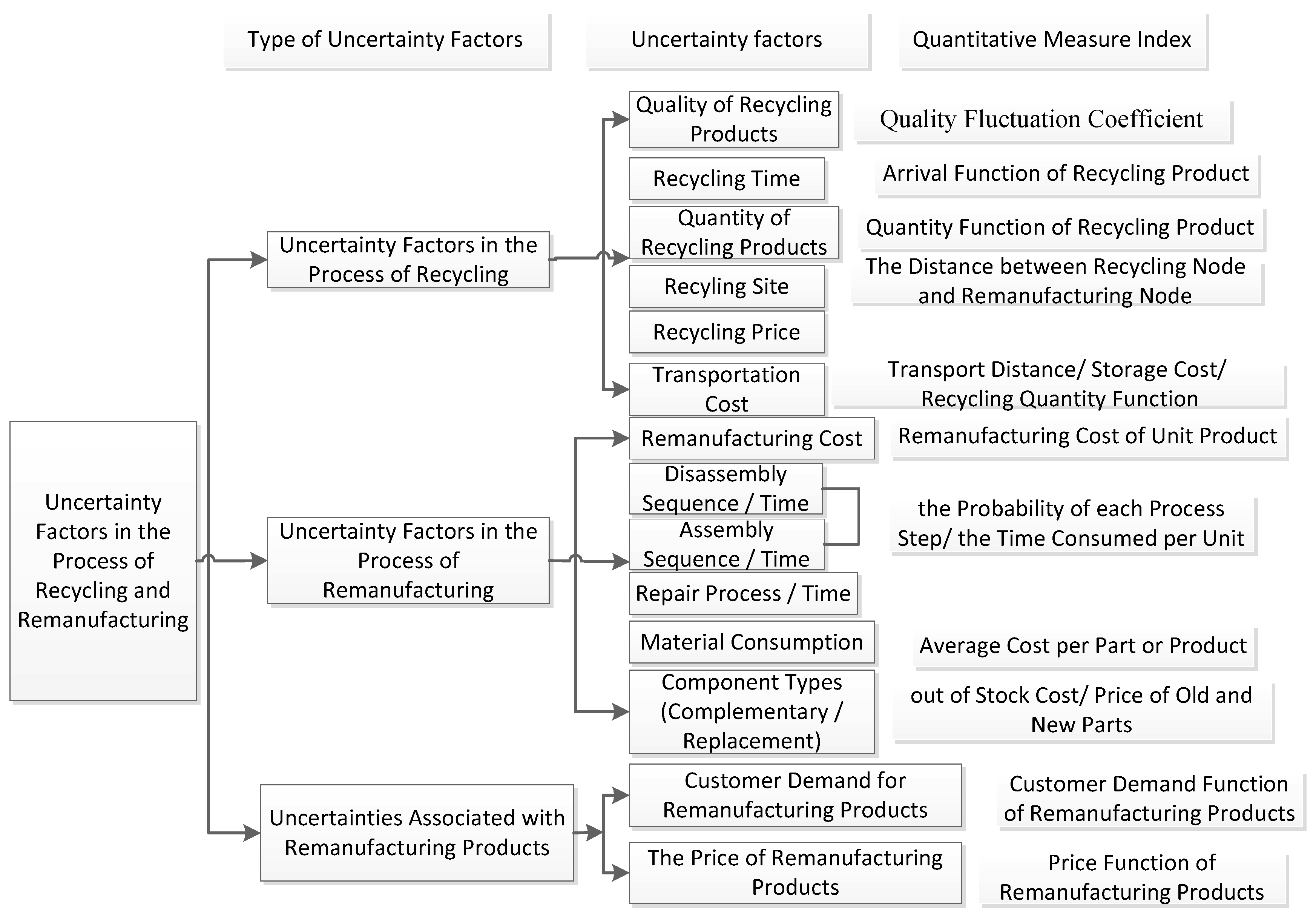
• Five uncertainty factors in remanufacturing process were taken into account in the model.
• The optimal recycling price and profits were obtained with maximization of resource benefits.
• Change regularity of resource benefits and profits were obtained as other factors varied.
• The study aims to provide government and manufacturers with decision support.
• These findings suggest that the uncertainty factors existing in remanufacturing can be controlled within a reasonable range.

1. Introduction

In recent decades, in order to decrease the costs and improve the utilization rate of resources and reduce the impacts on environment during the manufacturing processes, the remanufacturing of end-of-life (referred to as EOL in the rest of this article) products has experienced great development recently [1,2]. Though the remanufacturing industry in China is in its initial stage, it possesses great potential and rapid development speed. For example, in 2012, the automotive parts remanufacturing reached 8 billion Yuan and the reuse rate of recycled parts was 71.2%. Compared with new product manufacturing, remanufacturing can save the costs by more than 50%, energy consumption by 60%, materials consumption 70% and reduce the emissions by 80%, In recent years, the average annual growth rate of global remanufacturing industry reached 10%, the scale of the industry this year is expected to reach 250 billion Yuan, the quality and performance of remanufactured products can equal to or exceed over the new one, but its costs is only about 50% of them [3]. Furthermore, remanufacturing industry, as an important role of green economy, has been included in the “China manufacturing 2025” strategy. The Chinese government has formulated a series of policies, regulations and measures to promote it. Nonetheless, the remanufacturing processes of EOL construction machinery is a complicated system, which includes a series of processes such as delivering, cleaning, testing, disassembly, repairing, etc. [4]. The processes are accompanied with some uncertainty factors as quality, price, quantity of the recycled products, customer demands and their recognition to remanufactured products. Those factors do add the complexity of the resource benefits (including the energy benefits and the material benefits) evaluation during the remanufacturing processes of EOL construction machinery and cause additional costs and resource consumption. On the other hand, as a rational entity, the manufacturer, who wants to get more profits from remanufacturing, has to give greater consideration to the uncertainty factors in remanufacturing processes other than the resources and environmental benefits. These uncertainty factors in the remanufacturing processes add the difficulties to the evaluation of remanufacturing profits and environment benefits, therefore to calculate the maximum resource efficiency from the resource perspective becomes comparatively complicated but meaningful. For the government and remanufacturing enterprises, the common challenge is how to improve the resource benefits as much as possible under the constraints of ensuring the profits of the manufacturer.

The current research on evaluation of remanufacturing products are more focused on product design, logistics, sales models, and remanufacturing process. Among them that involving the uncertainty analysis are mainly about the pricing of EOL products, the economic evaluation of remanufacturing and the analysis of uncertainty factors existing in the benefits evaluation of EOL products.

(1) Research on price decision models [5] researched the remanufacturing and pricing strategies under uncertainty factors such as random yield and demand [6] studied the price decision, recycling policy and order strategy under the fixed and unfixed conditions of requirements and recovery rate [7] considered the joint pricing problem of new products and remanufactured products under uncertain demand and utilized the substitution of two product newsvendor models to solve the problem [8] develop and test a profits maximization model by simultaneously integrating recovery option selection and disassembly planning considering the quality of EOL components, and then develop an improved co-evolutionary algorithm (ICA) to search for an optimal EOL solution. The results show that the proposed approach offers a strong and flexible decision support tool for intelligent recovery management in a ubiquitous information environment.

(2) Research on the economic evaluation of remanufacturing. In the relevant literature about the economic evaluation of remanufacturing [9,10], respectively established decision models of used parts through different optimization algorithms, such as the recursive algorithm and genetic algorithm, in order to analyze the optimal scheme involving remanufacturing from technical and economic perspectives, and studied how to develop a recycling strategy when the supply and quality of recycled products are not determined [11] conducted an analysis on the economic viability of remanufacturing with the graph theoretic method, and obtained the maximum and minimum value of remanufacturing benefits [12] assessed the sustainability and maturity of remanufacturing enterprises from economic, environmental, and social dimensions. Several researchers explored the impacts of remanufacturing on resources and the environment through different models [13,14,15,16]. Based on a real disassembly of a passenger jet [17], develop a model to accurately evaluate the disassembly easiness of an airframe quantitatively incorporating both product and process features. In addition, the cutting and thrust force vectors are selected to evaluate and find the best operation sets. Such quantitative evaluation can help to proceed with a viable EOL strategy and implement newer approaches [18] model a retailer oriented closed-loop supply chain network for construction machinery remanufacturing and solve the network configuration with an improved genetic algorithm-based heuristic method to study the impact of collection ratio and capacity level on the configuration [19] examine the case of an automotive component manufacturer that wants to investigate product end of life (EOL) management, then estimate and create Sankey diagrams of the downstream flows of two components made of low-alloyed steel, to seek improvements in automotive EOL components [20] apply scenario-based hybrid Life Cycle Assessment(LCA) to calculate the economy-wide carbon footprints of seven electricity generation technologies.

(3) Research on the uncertainty factors in remanufacturing. The studies on uncertainty factors, which exist in remanufacturing processes, focused on the impact of remanufacturing on economic benefits, rather than ecological benefits (including resource benefits and environmental benefits) [21,22,23,24] made empirical analysis of critical elements of reverse logistics in Chinese manufacturing industry [13] studied the production and remanufacturing plan of manufacturers in a single cycle, and came to the conclusion: the lower the quality of the remanufactured product is, the higher the costs of the remanufacturing processes will be [25] found that there is a clear difference in customer preference as to whether to buy new or remanufactured products, after a study on the different consumption willingness of consumers between those two kinds of products [26] introduced the utility function into the remanufacturing system, and then studied the problem of the recycling price of EOL products under the stochastic demand and production rate [27] establish a decent model of a remanufacturer-driven closed-loop supply chain with multi-dimensional reverse channel within the framework of game theory, to characterize the uncertainty in the quality of collected used products for a closed-loop supply chain and give guidance to the construction machinery remanufacturing firms when facing with the quality uncertainty.

Most studies of existing literatures are focused on the analysis of uncertainty factors in remanufacturing or the economic evaluation of remanufacturing, yet little effort has been devoted to evaluating the resource benefits or the uncertainty factors which affect these [28,29]. Furthermore, although many related models on the remanufacturing process have acknowledged that remanufacturing does bring considerable benefits to resources [30,31,32], few of them have built a quantitative model to validate this proposition, or analyzed the internal evolution mechanism of remanufacturing resource benefits. In addition, the uncertainty factors accompanying remanufacturing processes, has brought a lot of challenges to the evaluation of the resource benefits of EOL products.

Considering the problems above and based on uncertainty of recycling price, to fill the gap of the lack of research on the quantification of environment and economic benefit evaluation for remanufacturing, this paper has not only constructed a quantitative model of resource benefits evaluation on remanufacturing processes of EOL construction machinery, but also made a mathematical analysis of recycling price and profits of remanufacturers under the maximization of resource benefits. Furthermore, the study in this paper has also covered the change regularity of resource benefits, recycling price and the profits of remanufacturers when recycling price, quality coefficient, requirement coefficient, and reusing ratio of products and parts are varying, and try to determine the equilibrium price, to provide relevant recommendations for enterprises and government, such as subsidies to the remanufacturers and appropriate marketing regulation of the recycling price, etc.

2. Model Establishing

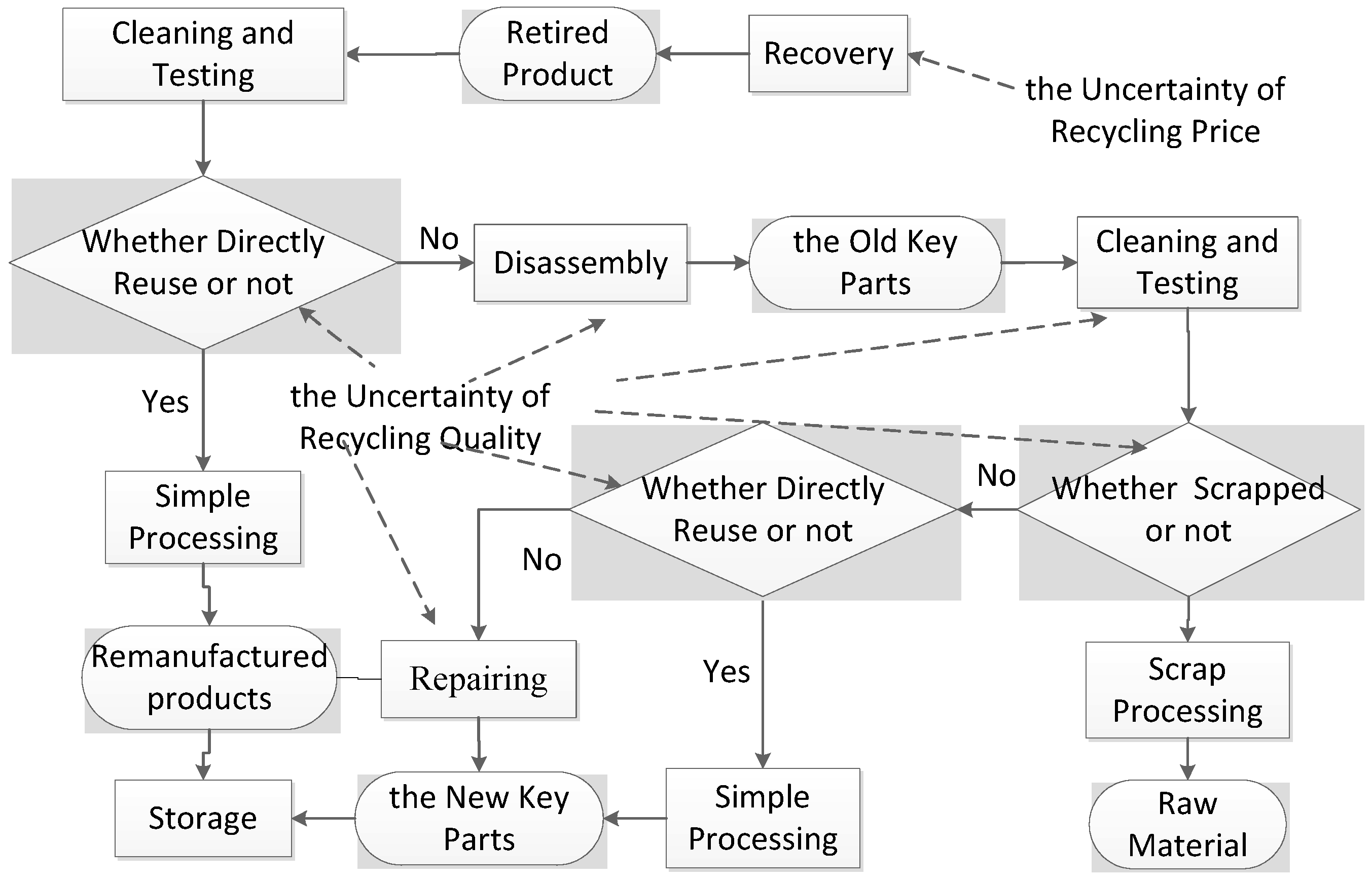
2.1. Problem Description

Construction machinery is a generic term for construction machines used in engineering construction such as architecture, water conservancy, electricity, roads, mines, ports, national defense and other fields. The working environment of these machines is relatively harsh compared to other kinds of machines [33].

After being recycled by factory at acquisition price, the EOL construction machinery will either be put into storage directly or disassembled into parts for use after going through the processes of cleaning and testing, remanufacturers put them into storage or on market after simple treatment, otherwise disassemble them into parts for use. As for those disassembled parts, they are to be scrapped, reused or repaired in accordance with the result of testing. If being scrapped, the parts are disposed and some of them will be recycled as raw material in terms of the standard program; those parts that are reusable will be directly put into storage or on market after simple treatment. Those processes are shown in Figure 1 below.

Figure 1 describes the remanufacturing processes of EOL construction machinery. According to the quality status of recycled products, the machine or its components are processed through two ways: reused directly or reused after repairing. By this measure, the remanufacturing processes of EOL construction machinery should be divided into three categories: (1) the machine can be reused directly; (2) the machine cannot be reused directly but its crucial components can be used after repairing; (3) neither the machine nor its crucial components can be remanufactured.

In the processes of recycling and remanufacturing, the uncertainties include recycling time, recycling quality, customer demand and their recognition on remanufactured products, these uncertainties lead to low efficiency and complexity for environment evaluation. In addition, with the different type and complex material composition of crucial components [34,35], they subsequently bring forth challenges to the efficiency of recycling and remanufacturing. These uncertainties not only cause a great waste of resources, but also affect the accuracy of government policy. It is necessary to establish a quantitative evaluation model for the remanufacturing processes to find out the potential uncertain factors and their intrinsic function mechanism for evaluating the resource benefits of remanufacturing.

According to the source of uncertainty in the remanufacturing system, in Section 2.1 we divide the uncertainties in recycling and remanufacturing into three categories: uncertainty in recycling, in remanufacturing and in new remanufactured products (no new products are taken into accounts). These uncertainty factors are presented in Figure 2.

In the processes of recycling and remanufacturing, the uncertainties of recycling time, recycling quality and customer demand lead to low efficiency and negative effects for remanufacturing. In addition, after the different types and complex material composition of crucial components are taken into accounts [34,35], the uncertainties in them will as well affect the overall efficiency of recycling and remanufacturing. EOL Based on Figure 2 and combined with the remanufacturing flowchart described in Figure 1, we choose five uncertainty factors (quality fluctuation coefficient, recycling price, demand coefficient, fill rate of customer demand, direct reusing rate of EOL construction machinery and reusing rate after repairing of crucial components) to establish the resource benefits model of remanufacturing processes.

2.2. Model Establishing

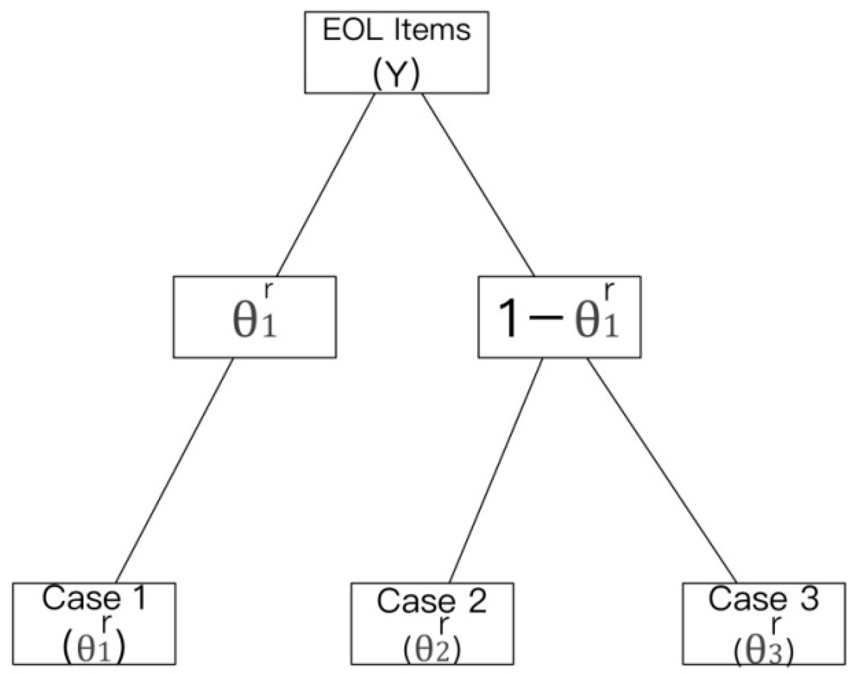
First, we define the variables with a set of concise and inerratic symbols. For the convenience of writing, we make some general rules for the symbols, such as C denotes costs ($C^a$ represents the costs for the acquisition of unit EOL item), P denotes profits ($P^m$ represents the unit profits in remanufacturing, $P^M$ represents the total profits for remanufacturing), $\mathsf{\alpha }$ denotes relationship (${\alpha }_Y^X$ denotes the relationship between customers’ demands $\mathrm{X}$ and the quantity of EOL products $Y$, i.e., demand satisfaction coefficient), $\theta$ denotes rate (${\theta }^g$ denotes the recognition rate of new remanufactured products by customers,), superscript p denotes processing, subscript i denotes in case i, e.g., $C_i^p$ denotes processing costs (cleaning, testing, disassembly, etc.) of unit EOL product in case i, ${\theta }_i^r$ denotes direct reuse rate of unit EOL product in case i, and $Q_{\ast }^m$ denotes the optimal quantity of manufactured cores, etc. The variables set in the model are listed in

Table 1. Uncertainty factors and their definition used in the model.

Parameters	Abbreviations	Definitions
X	The quantity of demands	The quantity of demands for new remanufactured products
Y	The quantity of acquisition	The quantity of returned EOL products
Case 1	$C_1$	When EOL construction machinery can be reused directly
Case 2	$C_2$	Not in Case 1, but its crucial components can be reused in remanufacturing after repairing
Case 3	$C_3$	Neither the product nor its crucial components can be remanufactured(not in Case 1 or Case 2)
$C^a$	Recycling price	Unit recycling price of EOL construction machinery
$C_i{}^P$	Processing costs	Processing costs(cleaning, testing, etc.) of EOL construction machinery in case i(i = 1,2,3)
$C_i{}^p$	Unit processing costs	Unit processing costs(cleaning, testing, etc.) of EOL construction machinery in case i(i = 1,2,3)
$C^d$	Unit disposal costs	Disposal costs of unit EOL product
$C^{un}$	Costs of uncertainty	Cost of uncertainty caused by EOL products quality
$C_L^{un}$, $C_R^{un}$	Left/Right end point	Left/Right end point of the interval of the uncertainty costs
${\alpha }^X$	The demand coefficient	The customer demand for remanufacturing products ($0\le {\alpha }^X\le 1$)
${\alpha }_Y^X$	Demand satisfaction coefficient	The relationship between customers’ demands $\mathrm{X}$ and the quantity of EOL products $\mathrm{Y}$
${\theta }_1^r$	Direct reusing rate of product in case 1	The direct reusing rate of EOL construction machinery in case 1 ($0\le {\theta }_1^r\le 1$)
${\theta }_2^r$	Direct reusing rate of components in case 2	The reusing rate after repairing of the crucial components in case 2 ($0\le {\theta }_2^r\le 1$)
${\theta }_3^r$	${\theta }_3^r=1-{\theta }_1^r-{\theta }_2^r$	The rate of the case does not belong to case1 or case or ($0\le {\theta }_3^r\le 1$)
${\theta }^q$	Recycling quality	The quality fluctuation coefficient ($0\le {\theta }^q\le 1$)
${\theta }^g$	Recognition coefficient	The recognition coefficient of new remanufactured products by customers
$P_i{}^U$	Resource net benefits	The overall resource benefits when the demand of customers are satisfied in case i(i = 1,2,3)
$P_i{}^u$	Unit net resource benefits	Unit resource benefits when the demand of customers are satisfied in case i(i = 1,2,3)
$P_i{}^M$	Net profits of reman	The profits of remanufacturers when the demand of customers are satisfied in case i(i = 1,2,3)
$P_i{}^m$	Unit net profits of reman	Profits of unit EOL item construction machinery in case i(i = 1,2,3), $P_i{}^m=(P_i{}^r-C_i{}^p-C^a)$
$P_i{}^r$	Unit profits of reman	Revenue of unit EOL item construction machinery in case i(i = 1,2,3)

.

According to the process analysis and characteristics of EOL product, the study in this paper made several assumptions as follows.

Assumption 1. There are $i$ kinds of crucial components in an EOL product and $j$ kinds of materials can be recycled in the remanufacturing processes.

Assumption 2. Remanufacturers do not participate in recycling process and only purchase them at price $C^a$, $C^a$ is defined as acquisition costs.

Assumption 3. The demand of new remanufactured product decreases with the rise of the selling price, and the selling price rises with the recycling price and the profits of remanufacturers $P^m$ ($P^m$denotes the revenue of unit EOL product). According to the equation of the relationship between customer demand and recycling price proposed by Li et al. in literature [5], we set the quantity of remanufacturing products that demanded by customers as $X=X_0\cdot {\theta }^g\cdot {\mathsf{\alpha }}^X\cdot {\left(C^a+P^m\right)}^{-\mathsf{\epsilon }}$ , here ${\mathsf{\alpha }}^X$ is demand coefficient$(0\le {\mathsf{\alpha }}^X\le 1)$ and it reflects the relationship between the market demand and the acquisition costs. ${\theta }^g$ is the recognition rate of new remanufactured products by customers, $X_0>0$ and $\mathsf{\epsilon }>1$ are constants representing the market scale and the price-elasticity index [5].

Assumption 4. The acquisition quantity of EOL products purchased by remanufacturers is proportional to the demand by customers, namely $Y={\theta }_Y^{X}X$, here ${\theta }_Y^X(0\le {\theta }_Y^X\le 1)$ is the fill rate of customer demand, this assumption is consistent with [5].

Assumption 5. The additional input caused by the uncertainty of products quality and crucial components brings negative benefits to resources, set the negative benefits as $C^{un}(C^{un}\ge 0)$; for the recycling price goes up with surplus value of EOL products in recycling process [22], so it is always reflected by product quality. When the recycling price is higher, the quality of EOL products is comparatively stable, and the value of $C^{un}$ is smaller [13]. Moreover, the value of $C^{un}$ is in an interval, namely $C^{un}\in (C_L^{un},C_R^{un})$ , here $C_L^{un}$ and $C_R^{un}$ represents the left end point and right end point of the interval respectively. The assumption of this interval conforms to the real situation of remanufacturing. Here we assume

$$C^{un}=\{\begin{array}{l}{a}_1-{\theta }^q\cdot C^a, \begin{array}{}\end{array}Whenanend-of-lifeconstructionmachinerycanbereuseddirectly\\ a_2-{\theta }^q\cdot C^a, Whentheend-of-lifeconstructionmachinerycannotbereuseddirectly,\\ but\mathrm{some}\mathrm{of}thecrucialcomponentscanbereused afterrepairing\\ a_3-{\theta }^q\cdot C^a, Neithertheproductnoritscrucialcomponentscanberemanufactured\end{array}$$

where $a_1$, $a_2$, $a_3$ are constants, which represent the upper limits of the additional resources inputting(due to the instability of the quality), and those three upper limit values can be obtained according to the historical data of the enterprise [36]. ${\theta }^q$ is the quality fluctuation coefficient$(0\le {\theta }^q\le 1)$; the greater the value of ${\theta }^q$ is, the better the quality status of EOL construction machinery, and the smaller the additional resources input in the remanufacturing processes will be.

When the market demand is satisfied in a single period, the overall resource benefits shall be set as $P^U$, the profits of remanufacturers as $P^M$. In this model, resource benefits is evaluated mainly from the perspectives of energy and materials, the resource benefits $P^U$ is consisted of energy benefits and material benefits. There are three cases in Figure 1, then the resource benefits and the profits of remanufacturer can be divided into three parts as Figure 2 shows:

Case 1:

When EOL construction machinery can be reused directly, $P_1^U$ and $P_1^M$ represent the remanufacturing resource benefits and the profits of remanufacturer.

Case 2:

When EOL construction machinery cannot be reused directly while its crucial components can be reused after repairing, $P_2^U$ and $P_2^M$ denote the remanufacturing resource benefits and the profits of remanufacturer.

Case 3:

Neither the product nor its crucial components can be remanufactured, $P_3^U$ and $P_3^M$ represent the remanufacturing resource benefits and the profits of remanufacturer. This is reasonable in practice. When recycling EOL products, the remanufacturer usually set certain requirements and only products above the condition threshold are recycled or remanufactured. The rates of these three cases are shown as Figure 3.

For case i, the overall resource benefits is $P_i{}^U=Y\cdot {\theta }_i^r\cdot P_i{}^u=Y\cdot {\theta }_i^r\cdot \left(P_i{}^e+P_i{}^l-C_i{}^{un}\right)$, the profits of remanufacturers is $P_i{}^M=Y\cdot {\theta }_i^r\cdot P_i{}^m=Y\cdot {\theta }_i^r\cdot \left(P_i{}^r-C_i^p-C^a\right)$, i = 1, 2, 3, here $P_i{}^e$ is the energy saving of unit EOL product in case i, $P_i{}^l$ is the material saving of unit EOL product in case i.

Case 1: When EOL construction machinery can be reused directly.

$C_1{}^p$ denotes the processing costs(cleaning, testing, etc.) of unit EOL construction machinery in Case 2, $P_1{}^m$ the net profits of unit EOL construction machinery.

$$\begin{array}{l}{P}_1{}^U=Y\cdot {\theta }_1^r\cdot P_1{}^u={\mathsf{\alpha }}_Y^{X}X\cdot {\theta }_1^r\cdot \left(P_1{}^e+P_1{}^l+P_1{}^{\theta }-C_1{}^{un}\right)\\ =X_0{\mathsf{\alpha }}_Y^X{\alpha }^X{\theta }^g{\left(C^a+P^r\right)}^{-\mathsf{\epsilon }}\cdot {\theta }_1^r\cdot (z{p}_{\mathrm{m}}+{\displaystyle \sum _i{x}_i{}^2{p}_m}+{\displaystyle \sum _i{\displaystyle \sum _j{m}_{ij}{p}_j{}^2+{\displaystyle \sum _i{\displaystyle \sum _j{m}_{ij}{x}_j{}^1{p}_m-C_1{}^{un})}}}}\end{array}$$

(1)

$$P_1{}^M=Y\cdot {\theta }_1^r\cdot P_1{}^m=X_0{\mathsf{\alpha }}_Y^X{\theta }^g{\mathsf{\alpha }}^X{\left(C^a+P_1{}^r\right)}^{-\mathsf{\epsilon }}\cdot {\theta }_1^r\cdot (P_1{}^r-C_1{}^p-C^a)$$

(2)

Where $P_1^e=z{p}_{\mathrm{m}}+{\displaystyle \sum _i{x}_i{}^2{p}_m}$ denotes the energy saving of unit EOL product in case 1, $z{p}_{\mathrm{m}}$ represents the energy profits brought by the reduction of assembly processes in remanufacturing and ${\displaystyle \sum _i{x}_i{}^2{p}_m}$ represents the energy benefits brought by the reduction of manufacturing processes in remanufacturing; $P_1{}^{\theta }={\displaystyle \sum _i{\displaystyle \sum _j{m}_{ij}{p}_j{}^2+{\displaystyle \sum _i{\displaystyle \sum _j{m}_{ij}{x}_j{}^1{p}_m}}}}$ denotes the material profits of unit EOL product in case 1, in which $P_1{}^l={\displaystyle \sum _i{\displaystyle \sum _j{m}_{ij}{p}_j{}^2}}$ represents the material benefits brought by the direct reusing of key parts in remanufacturing; ${\displaystyle \sum _i{\displaystyle \sum _j{m}_{ij}{x}_j{}^1{p}_m}}$ represents the resource benefits brought by the material savings of key parts in remanufacturing; $C_1{}^{un}=a_1-{\theta }^q\cdot C^a$ represents the additional input of material and energy caused by the uncertainty in quality of products and crucial components. $P_1{}^t-C_1^p-C^a$ represents the profits obtained from unit EOL construction machinery product in case 1.

Case 12 When the EOL construction machinery cannot be reused directly, but some of its crucial components can be reused in remanufacturing after repairing.

Let $C_2^p$ denote processing costs(cleaning, testing, disassembly, etc.) of unit EOL construction machinery and its crucial components in case 2, $v_i^1$ denote profits obtained by remanufacturers from the $i$th crucial component of unit EOL construction machinery, $w_j^1$ denote profits obtained by remanufacturers from the$j$th recyclable material of unit EOL construction machinery, $C^d$ denote disposal costs of unit EOL product. The remanufacturing resource benefits $U_2$ and the profit of remanufacturer $M_2$ are:

$$\begin{array}{ll}{P}_2{}^U& =Y\cdot {\theta }_2^r\cdot P_2{}^u={\mathsf{\alpha }}_Y^{X}X\cdot {\theta }_2^r\cdot \left(P_2{}^e+P_2{}^l+P_2{}^{\theta }-C_2{}^{un}\right)\\ & =X_0{\mathsf{\alpha }}_Y^X{\alpha }^X{\theta }^g{\left(C^a+P^t\right)}^{-\mathsf{\epsilon }}\cdot {\theta }_2^r\cdot ({\displaystyle \sum _i{x}_i{}^2{p}_m}+{\displaystyle \sum _i{\displaystyle \sum _j{m}_{ij}{p}_j{}^2+{\displaystyle \sum _i{\displaystyle \sum _j{m}_{ij}{x}_j{}^1{p}_m-C_2{}^{un})}}}}\end{array}$$

(3)

$$P_2{}^M=Y\cdot {\theta }_2^r\cdot P_2{}^m=X_0{\mathsf{\alpha }}_Y^X{\theta }^g{\mathsf{\alpha }}^X{\left(C^a+P_2{}^r\right)}^{-\epsilon }\cdot {\theta }_2^r\cdot ({\displaystyle \sum _i{v}_i^1+{\displaystyle \sum _j{w}_j^1-C_2^p-C_2^d-C^a)}}$$

(4)

Where ${\displaystyle \sum _i{x}_i{}^2{p}_m}$ represents the energy benefits brought by the reduction of manufacturing processes in remanufacturing; $P_2{}^l={\displaystyle \sum _i{\displaystyle \sum _j{m}_{ij}{p}_j{}^2}}$ represents the material benefits brought by the direct reusing of key parts in remanufacturing; $P_2{}^{\theta }={\displaystyle \sum _i{\displaystyle \sum _j{m}_{ij}{x}_j{}^1{p}_m}}$ represents the resource benefits brought by the material savings of key parts in remanufacturing; $C_2{}^{un}$ represents the additional input of material and energy caused by the uncertainty in quality of products and crucial components; $P_2{}^m={\displaystyle \sum _i{v}_i^1+{\displaystyle \sum _j{w}_j^1-C_2^p-C_2^d-C^a}}$ represents the net profits obtained from unit EOL product.

Case 3: Neither the product nor its crucial components can be remanufactured.

Let $C_2{}^p$ denote processing costs (cleaning, testing, disassembly, EOL disposal, etc.) of unit EOL product and its crucial components, $w_j^2$ denote profit obtained from the $j$th recyclable material of unit EOL product, $C_3^d$ denote disposal costs of unit EOL product. The remanufacturing resource benefits $P_3^U$ and the profits of remanufacturer $P_3^M$ are:

$$\begin{array}{ll}{P}_3{}^U& =Y\cdot {\theta }_3^r\cdot P_3{}^u={\alpha }_Y^{X}X\cdot {\mathsf{\theta }}_3^r\cdot \left(P_3{}^e+P_3{}^l+P_3{}^{\theta }-C_3{}^{un}\right)\\ & =X_0{\mathsf{\alpha }}_Y^X{\alpha }^X{\theta }^g{\left(C^a+P^t\right)}^{-\epsilon }\cdot {\theta }_3^r\cdot ({\displaystyle \sum _i{\displaystyle \sum _j{m}_{ij}{p}_j{}^2+{\displaystyle \sum _i{\displaystyle \sum _j{m}_{ij}{x}_j{}^1{p}_m-C_3{}^{un})}}}}\end{array}$$

(5)

$$P_3^M=Y\cdot {\theta }_3^r\cdot P_3{}^m=X_0{\mathsf{\alpha }}_Y^X{\theta }^g{\mathsf{\alpha }}^X{\left(C^a+P_3{}^r\right)}^{-\mathsf{\epsilon }}\cdot {\theta }_3^r\cdot ({\displaystyle \sum _j{w}_j^2-C_3^p-C_3^d-C^a)}$$

(6)

Where ${\displaystyle \sum _i{\displaystyle \sum _j{m}_{ij}{x}_j{}^1{p}_m}}$ represents the resource benefits brought by the material savings of key parts in remanufacturing; ${\displaystyle \sum _i{x}_i{}^2{p}_m}$ represents the energy benefits brought by the reduction of manufacturing processes in remanufacturing; ${\displaystyle \sum _i{\displaystyle \sum _j{m}_{ij}{p}_j{}^2}}$ represents the material benefits brought by the direct reusing of key parts in remanufacturing; $C_3{}^{un}$ represents the additional input of material and energy caused by the uncertainty in quality of products and crucial components. $P_3{}^m={\displaystyle \sum _j{w}_j^2-C_3^p-C_3^d-C^a}$ represents the profits obtained from unit EOL construction machinery product.

Therefore, let $P^U=P_{{}_1}^U+P_{{}_2}^U+P_{{}_3}^U$ and $P^U=P_{{}_1}^M+P_{{}_2}^M+P_{{}_3}^M$, functions of the resource benefits and remanufacturer profits brought by remanufacturing are as follow:

$$\begin{array}{ll}\max P^U=& X_0{\mathsf{\alpha }}_Y^X{\alpha }^X{\theta }^g{\left(C^a+P^r\right)}^{-\mathsf{\epsilon }}\cdot {\theta }_1^r\cdot (z{p}_{\mathrm{m}}+{\displaystyle \sum _i{x}_i{}^2{p}_m}+{\displaystyle \sum _i{\displaystyle \sum _j{m}_{ij}{p}_j{}^2+{\displaystyle \sum _i{\displaystyle \sum _j{m}_{ij}{x}_j{}^1{p}_m-C_1{}^{un})}}}}+\\ & X_0{\mathsf{\alpha }}_Y^X{\alpha }^X{\theta }^g{\left(C^a+P^t\right)}^{-\mathsf{\epsilon }}\cdot {\theta }_2^r\cdot ({\displaystyle \sum _i{x}_i{}^2{p}_m}+{\displaystyle \sum _i{\displaystyle \sum _j{m}_{ij}{p}_j{}^2+{\displaystyle \sum _i{\displaystyle \sum _j{m}_{ij}{x}_j{}^1{p}_m-C_2{}^{un})}}}}+\\ & X_0{\mathsf{\alpha }}_Y^X{\alpha }^X{\theta }^g{\left(C^a+P^t\right)}^{-\mathsf{\epsilon }}\cdot {\theta }_3^r\cdot ({\displaystyle \sum _i{\displaystyle \sum _j{m}_{ij}{p}_j{}^2+{\displaystyle \sum _i{\displaystyle \sum _j{m}_{ij}{x}_j{}^1{p}_m-C_3{}^{un})}}}}\end{array}$$

(7)

$$\begin{array}{ll}\max \underset{P^U\to P_{{}_{\max }}^U}{P^M}& =Y\cdot {\theta }_1^r\cdot P_1{}^m=X_0{\mathsf{\alpha }}_Y^X{\theta }^g{\mathsf{\alpha }}^X{\left(C^a+P_1{}^r\right)}^{-\mathsf{\epsilon }}\cdot {\theta }_1^r\cdot (P_1{}^r-C_1^p-C^a)+\\ & Y\cdot {\theta }_2^r\cdot P_2{}^m=X_0{\mathsf{\alpha }}_Y^X{\theta }^g{\mathsf{\alpha }}^X{\left(C^a+P_2{}^r\right)}^{-\mathsf{\epsilon }}\cdot {\theta }_2^r\cdot ({\displaystyle \sum _i{v}_i^1+{\displaystyle \sum _j{w}_j^1-C_2^p-C_2^d-C^a)}}+\\ & Y\cdot {\theta }_3^r\cdot P_3{}^m=X_0{\mathsf{\alpha }}_Y^X{\theta }^g{\mathsf{\alpha }}^X{\left(C^a+P_3{}^r\right)}^{-\mathsf{\epsilon }}\cdot {\theta }_3^r\cdot ({\displaystyle \sum _j{w}_j^2-C_3^p-C_3^d-C^a)}\end{array}$$

(8)

The definition of parameters used in Equations (7) and (8) are as follows:

$x_j{}^1$ denotes the energy consumption when producing a unit of the $j$th recycling material (converted into standard coal); $p_m$ denotes the market price of standard coal; $p_j{}^2$ denotes the market price of the $j$th recycling material. $x_i{}^2$ denotes the energy consumption when producing the $i$th crucial component; $z$ denotes the energy consumption during the assembling process of a unit product. $m_{ij}$ denotes the consumption of the $j$th recycling material when producing the $i$th crucial component. $C_i{}^p(i=1,2,3)$ denotes processing costs(cleaning, testing, disassembly, disposal, etc.). According to the actual operation in remanufacturing enterprises, set $C_i^p$ as a step function of the quality fluctuation coefficient ${\theta }^q$. For example, when ${\theta }^q$ varies in the interval [0.1–0.2], the value of $C_i^p$ is $C_1^p$; when ${\theta }^q$ varies in the interval [0.3–0.6], the value of $C_i^p$ is $C_2^p$ , where $C_1^p$ and $C_2^p$ are constants. Let the rate of the direct reusing of EOL construction machinery be ${\theta }_1^r(0\le {\theta }_1^r\le 1)$; the reusing rate after repairing of the crucial components be ${\theta }_3^r(0\le {\theta }_3^r\le 1)$.

$$\text{Constraints}: \mathrm{s} .\mathrm{t}. \{\begin{array}{ll}{C}_3^p\ge C_2^p\ge C_1^p>0& \hfill (9)\\ v_i^1>0& \hfill (10)\\ w_j^1\ge w_j^2>0& \hfill (11)\\ C_3^d\ge C_2^d>0& \hfill (12)\\ a_1,a_2,a_3,{\theta }^q,C^a,{\alpha }^X all are bigger than 0& \hfill (13)\end{array}$$

For the constraints, constraint (9) represents the non-negative costs constraints in these three remanufacturing cases above; Constraint (10) represents the benefits constraint of the ith component in the case that the EOL construction machinery cannot be reused directly, but some of its key components can be reused after repairing; Constraint (11) represents the non-negative benefits constraint; Constraint (12) represents the costs constraint of waste disposal.

Obviously, many parameters, including constants and variables, are defined in this model. The values of those constants can be obtained through the survey on the actual operations in remanufacturing factories. However, the forecast values of the variables are obtained through some statistical methods. For example, the forecast values of the variables are obtained through some statistical methods, the demands of current period are unknown but predicable, for the demands of past periods are known, then by using moving average method we can predicate the demands of current period. Set the annual demands of customers be $M_t$ ($t$ denotes the number of year), $n$ denotes the number of periods. Then the demands predictions of current period $a_{t+1}$ can be obtained by the expression as follow:

$$a_{t+1}=M_t^{\left(1\right)}=\frac{a_t+a_{t-1}+\dots +a_{t-n}}{n}$$

(14)

3. Model Solving

When taking the derivative of objective function, let $\partial P^U/\partial C^a=0$, then we get $C_{\ast }^a$, $P^U$ get the maximum value at this point (refer to Appendix A for the detailed solving process). When the recycling price of EOL construction machinery is $C_{\ast }^a$, the overall resource benefits $P^U$ brought by remanufacturing reach a maximum, and then the demands of customers can be decided accordantly. When $C^a\le C_{\ast }^a$ , the resource benefits $P^U$ increases with recycling price $C^a$, when $C^a\ge C_{\ast }^a$ , $P^U$ decreases with the increasing of $C^a$. However, when $C^a=C_{\ast }^a$, whether the value of $P_1^M$, is positive or negative is unknown. Therefore, further analysis of profits function is needed to find the relationship between profits and the recycling price.

Set $\partial P^M/\partial C^a=0$, if $C^a=\frac{\mathsf{\epsilon }(l-d)-P^r}{(\mathsf{\epsilon }+1)}=C_{\ast \ast }^a$, the profits in a single period reaches its minimum at this point, $P_{\min }^M=X_0{\theta }_Y^X{\theta }^g{\alpha }^X\left[\frac{l-d-P^r}{\mathsf{\epsilon }+1}\right]{\left[\frac{l^{\prime }+{\theta }^q{P}^r}{{\theta }^q(\mathsf{\epsilon }-1)}\cdot \mathsf{\epsilon }\right]}^{-\mathsf{\epsilon }}$. Obviously, when $P_{\min }^M$ < 0, the marginal profits is zero for remanufacturers, it means the remanufacturing is unprofitable and it is impossible to continue. Therefore, the optimal solution $C_{\ast \ast }^a$ is an invalid solution, but with overall profits function being taken into account, the conclusion can be drew as: when $C^a\le C_{\ast \ast }^a$, $P^U$ is increasing with the decreasing of $C^a$; when $C^a\ge C_{\ast \ast }^a$, $P^U$ increases with the increasing of $C^a$ (here government subsidies for remanufacturing companies are not taken into consideration) .

The conclusion drawn by taking the derivative of $P^U$ and $P^M$ shows that the impact on remanufacturer’s profits and resource benefits imposed by recycling price, on this basis, further analysis for the plus or minus of profits and benefits is needed.

By $\{\begin{array}{l}{P}^U=Y\cdot (l^{\prime }+{\theta }^q{C}^a)\\ P^M=Y\cdot (l-d-C^a)\end{array}$ and set $P^M$ equals zero, then we get $C^a=l-d$; set $P^U$ equals zero, then $C^a=\frac{-l^{\prime }}{b}$.

Therefore, for $P^M\left(C^a\right)\ge 0$, meet the condition $C^a\le l-d$. Meanwhile, for $P^U\left(C^a\right)\ge 0$, meet $C^a\ge \frac{-l^{\prime }}{b}$. When $P^M\left(C^a\right)\ge 0$ and $P^U\left(C^a\right)\ge 0$, based on the above inequalities, the conclusion can be drawn as follows:

When $C_{\ast }^a$ meet the following conditions, then for any $C_{\ast }^a$, the model satisfies $P^U\left(C_0^a\right)\ge 0$ and $P^M\left(C_0^a\right)\ge 0$. That is $C_0^a\in \left[0,l-d\right]$.

In the actual production process, the raw material and energy consumed by unit product or component, the prices of raw material and unit standard coal are known, namely the value of $d$, $l$, $l^{\prime }$ are fixed. If there is recycling price ${\mathrm{p}}_0$ to make $P^U\left(C_0^a\right)\ge 0$ and $P^M\left(C_0^a\right)\ge 0$, then the value of $C_0^a$ is dependent on the quality fluctuation ${\theta }^q$, the direct reusing rate of EOL construction machinery ${\theta }_1^r$ and the reusing rate of the crucial components ${\theta }_2^r$.

From the description above we can draw the conclusion as that: in the process of recycling EOL products, once the quality of products is confirmed, namely the quality fluctuation coefficient, the rate of the direct reusing of EOL machinery and its component are determined, and then the recycling price can be determined. Conversely, with the actual recycling price, it is feasible to choose EOL products of better quality (the quality fluctuation coefficient ${\theta }^q$ is larger) from recycling merchants.

The expression of the resource benefits $P^M$, the profits of remanufacturer $P^U$ and the recycling price $C^a$ contain not only many variables that represents uncertainty factors, such as ${\mathsf{\alpha }}_Y^X$, ${\theta }^g$, ${\mathsf{\alpha }}^X$, ${\theta }^q$, ${\theta }_1^r$, ${\theta }_2^r$, ${\theta }_3^r$, but also a lot of constants, like $m_{ij}$, $z$, $j$, $p_j{}^2$. Once we get the exact values of these constants and variables, the value of $P^U$, $P^M$ and $C^a$ can be quickly obtained according to the expression. In the actual remanufacturing activities, some of those parameters can be obtained directly through the survey in the remanufacturing factory, and some other parameters can be obtained by using some statistical methods (such as moving average method, exponential smoothing method) to deal with the historical data of the remanufacturing enterprise.

4. Impact Analysis of the Uncertainty Factors

In this model, the fill rate of customer demands ${\mathsf{\alpha }}_Y^X$, the recognition coefficient of new remanufactured products from customers ${\theta }^g$, the quality fluctuation coefficient ${\theta }^q$, customer demands ${\alpha }^X$, the direct reusing rate of EOL products ${\theta }_1^r$ and the reusing rate after repairing of the crucial components ${\theta }_2^r$, those all have different impact on the resource benefits maximum $P_{\ast }^U$, the recycling price $C_{\ast }^a$ and profits of remanufacturers $P_1^M$ under the maximization of resource benefits. However, the extent to which they have an impact needs to be further analyzed.

4.1. Analysis of the Uncertainty Factors Associated with Customer Demand

The demand for remanufacturing products is directly reflected by customer demands coefficient ${\alpha }^X$, the fill rate of customer demands ${\alpha }_Y^X$ and the recognition coefficient of new remanufactured products from customers ${\theta }^g$. They exert significant influence on remanufacturers profits and resource benefits during remanufacturing processes; Based on mathematic expression as follows:

$$\{\begin{array}{l}{P}_{\ast }^U=X_0{\alpha }_Y^X{\theta }^g{\alpha }^X\frac{{\theta }^q{P}^r-l^{\prime }}{\epsilon -1}{\left[\frac{\epsilon l^{\prime }+{\theta }^q\epsilon P^r}{{\theta }^q(\epsilon -1)}\right]}^{-\epsilon }\\ P_1^M=\frac{{\theta }^q{P}^r-l^{\prime }}{\epsilon -1}\left[(\mathrm{l}-\mathrm{d})-\frac{{\theta }^q{P}^r-l^{\prime }}{\epsilon -1}\right]{\left[\frac{\epsilon l^{\prime }+{\theta }^q\epsilon P^r}{{\theta }^q(\epsilon -1)}\right]}^{-\epsilon }\\ C_{\ast }^a=\frac{{\theta }^q{P}^r-\epsilon l^{\prime }}{{\theta }^q(\epsilon -1)}\end{array}\sqrt{{({\theta }^q)}^2-4ac}$$

(15)

The demand coefficient ${\alpha }^X$, the fill rate of customer demands ${\alpha }_Y^X$ and the recognition coefficient of new remanufactured products from customers ${\theta }^g$ are proportional to the resource benefits and the profits of remanufacturers, while they have no effect on recycling price. In other words, the higher the recognition degree and fill rate of customer demands are, the larger the resource benefits of remanufacturing and the profits of remanufacturers are becoming.

Meanwhile, in the actual process of remanufacturing, the fill rate of customer demands ${\alpha }_Y^X$ in current period is often influenced by other periods, and it may also bring a measure of influence on the fill rate of customer demands in upcoming periods. Therefore, it is necessary to make analysis for ${\alpha }_Y^X$ in multi-period.

As for manufacturing enterprises, the customer demand changes during different periods will bring a measure of influence on the allocation of production resources and manufacturing adjustment, and whether the demands of current period are satisfied also has effects on how the demands are satisfied during next period. Here we assume when the demands during current period are satisfied, then in next period the probability that the demands are satisfied is $\delta$; when the demands during current period are not satisfied, then in next period the probability that the demands are satisfied is $\sigma$. Meanwhile, whether the demands are satisfied in next period is independent on previous events, only related to current state.

The remanufacturing system above makes up a two-state Markov chain (please refer to Appendix B for the detailed solving process). By solving the chain Markov, we can conclude that under such condition whether the demand in the next period are satisfied or not is independent on previous state and only related to current state, the limiting probability about customer demands satisfaction converges to a fixed value $\frac{\sigma }{1+\sigma -\delta }$ and is independent on the state of current period.

Despite its great difficulty and lower accuracy when predicting the customer demands during a long term according to historical data, the limiting probability of the fill rate for customer demands converges to a fixed value. Where $\delta$ and $\sigma$ can be obtained by the statistical remanufacturers business data, here it is taken as a constant. Therefore, it serves as a reference for the remanufacturers who want to predict the long term demands of customers.

4.2. Analysis of the Quality Fluctuation Coefficient

The quality fluctuation coefficient $b$ denotes the quality condition of recycled EOL construction machinery and its crucial components, the value of ${\theta }^q$ determines the impact on environment and resource input during the process of remanufacturing. Therefore, to make analysis of ${\theta }^q$ is becoming important and meaningful.

In analysis of previous section, Equation (15) has shown that the quality fluctuation coefficient ${\theta }^q$ exerts significant influence on the value of $P_{\ast }^U$, $P_1^M$ and $C_{\ast }^a$, but the specific impact of ${\theta }^q$ on $P_{\ast }^U$, $P_1^M$ and $C_{\ast }^a$ remain to be further analyzed.

Please refer to Appendix C for the detailed solving process, from the result of solving process, we can get, there is ${\theta }_{\ast }^q$, When ${\theta }_{\ast }^q=\frac{l^{\prime }\epsilon }{P^r(\epsilon -1)}$, the resource benefit $P^U$ reaches its minimum. Moreover, when ${\theta }^q\le {\theta }_{\ast }^q$, $P^U$ decreases with the increasing of ${\theta }^q$; when ${\theta }^q\ge {\theta }_{\ast }^q$, it increases with the increasing of ${\theta }^q$.

From the expression of ${\theta }_{\ast }^q$ we can draw the conclusion: when the resource benefits is minimum, the value of quality fluctuation coefficient ${\theta }_{\ast }^q$ is related to $l^{\prime }$, and ${\theta }_{\ast }^q$ is proportional to $l^{\prime }$. According to the previous definition, $l^{\prime }$ is a function of the direct reusing rate of EOL products ${\theta }_1^r$ and the reusing rate after repairing of the crucial components ${\theta }_2^r$ , that is to say, ${\theta }_1^r$ and ${\theta }_2^r$ directly decide the value of ${\theta }_{\ast }^q$. Therefore, once the impact of ${\theta }_2^r$ and ${\theta }_2^r$ on $l^{\prime }$ are recognized, the change regularity of ${\theta }_{\ast }^q$ on the condition that when ${\theta }_1^r$ and ${\theta }_2^r$ are varying can be got (further analysis has been made in Section 4.3). Meanwhile, the expression of ${\theta }_{\ast }^q$ shows the larger the profits of remanufacturer $P^r$ and the price-elasticity index $\epsilon$ are, the smaller the value of ${\theta }_{\ast }^q$ will be. Therefore, when recycling the EOL construction products, remanufacturers should choose those products that their quality is comparatively low but the parts of them can be reused directly, which can ensure not only low recycling price but also larger quantity of reusable parts to increase the remanufacturing profits.

4.3. Analysis of the Direct Reusing Rate of EOL Product and Its Components

By $\{\begin{array}{l}{l}^{\prime }={\theta }_3^r({\displaystyle \sum _i{\displaystyle \sum _j{m}_{ij}{p}_j{}^2+{\displaystyle \sum _i{\displaystyle \sum _j{m}_{ij}{x}_j{}^1{p}_m-a_1)+}}}}{\theta }_2^r({\displaystyle \sum _i{\displaystyle \sum _j{m}_{ij}{p}_j{}^2+}}\\ \begin{array}{}\end{array}{\displaystyle \sum _i{\displaystyle \sum _j{m}_{ij}{x}_j{}^1{p}_m+{\displaystyle \sum _i{x}_i{}^2{p}_m-a_2})}}+{\theta }_1^r(z{p}_m+{\displaystyle \sum _i{\displaystyle \sum _j{m}_{ij}{p}_j{}^2+{\displaystyle \sum _i{\displaystyle \sum _j{m}_{ij}{x}_j{}^1{p}_m+{\displaystyle \sum _i{x}_i{}^2{p}_m}-a_3)}}}}\\ l={\theta }_3^r{\displaystyle \sum _j{w}_j^2+}{\theta }_2^r({\displaystyle \sum _i{v}_i^1+{\displaystyle \sum _j{w}_j^1)+}}{\theta }_1^r{P}^r\\ d={\theta }_3^r(C_3^p+C_3^d)+{\theta }_2^r(C_2^p+C_2^d)+{\theta }_1^r{C}_1^p\end{array}$ and the expressions of $P_{\ast }^U$ and $P_1^M$ we get Equation (15):

As a matter of convenience in follow-up analysis, here $l^{\prime }$, $l$ and $d$ are parameters as resource benefits of unit remanufacturing product, profits and costs of unit remanufacturing product.

From Equation (15) it can be concluded that ${\theta }_1^r$ and ${\theta }_2^r$ finally exert influence on $P_1^M$, $X_{\ast }$and $C_{\ast }^a$ by affecting parameters of $l^{\prime }$, $l$ and $d$. Considering the parameters of $l$, $l^{\prime }$ and $d$ defined in this model have some special meanings, which represent profits of unit remanufacturing product, total resource benefits and costs of unit remanufacturing product, here we first analyze the impact that $l$, $l^{\prime }$ and $d$ have on the optimal values of $P_{\ast }^U$, $P_1^M$, $X_{\ast }$ and $C_{\ast }^a$, then the impact that ${\theta }_i^r$ have on $l$, $l^{\prime }$ and $d$, which is more meaningful than iterating ${\theta }_i^r$ directly into the optimal values.

For the impacts of $l$, $l^{\prime }$ and $d$ on the optimal values, please refer to Appendix D.1 for detailed solving process.

For the impacts of ${\theta }_i^r$ on $l$, $l^{\prime }$ and $d$, please refer to Appendix D.2 for detailed solving process.

Therefore, according to the solving result in Appendix D, the conclusion can be drawn as follows:

(1) When ${\phi }_3<\frac{{\theta }_3^r}{1-{\theta }_1^r}{\phi }_1+\frac{{\theta }_2^r}{1-{\theta }_1^r}{\phi }_2$, $l^{\prime }$ increases with ${\theta }_1^r$; when ${\phi }_3>\frac{{\theta }_3^r}{1-{\theta }_1^r}{\phi }_1+\frac{{\theta }_2^r}{1-{\theta }_1^r}{\phi }_2$, $l^{\prime }$ decreases with the increase of ${\theta }_1^r$ ; when ${\phi }_3=\frac{{\theta }_3^r}{1-{\theta }_1^r}{\phi }_1+\frac{{\theta }_2^r}{1-{\theta }_1^r}{\phi }_2$ , $l^{\prime }$ is independent on${\theta }_1^r$ ; when${\phi }_1<{\phi }_2$, $l^{\prime }$ increases with ${\theta }_3^r$; when ${\phi }_1>{\phi }_2$, $l^{\prime }$ decreases with the increase of ${\theta }_2^r$; when ${\phi }_1={\phi }_2$, $l^{\prime }$ is independent on ${\theta }_2^r$.

(2) When ${\mu }_3<\frac{{\theta }_3^r}{1-{\theta }_1^r}{\mu }_1+\frac{{\theta }_2^r}{1-{\theta }_1^r}{\mu }_2$, $d$ increases with ${\theta }_1^r$; when ${\mu }_3>\frac{{\theta }_3^r}{1-{\theta }_1^r}{\mu }_1+\frac{{\theta }_2^r}{1-{\theta }_1^r}{\mu }_2$, $d$ decreases with the increase of ${\theta }_1^r$; when ${\mu }_3=\frac{{\theta }_3^r}{1-{\theta }_1^r}{\mu }_1+\frac{{\theta }_2^r}{1-{\theta }_1^r}{\mu }_2$, $d$ is independent on ${\theta }_1^r$; when ${\mu }_1<{\mu }_2$, $d$ increases with ${\theta }_2^r$; when ${\mu }_1>{\mu }_2$, $d$ decreases with the increase of ${\theta }_2^r$; when ${\mu }_1={\mu }_2$, $d$ is independent on ${\theta }_2^r$.

(3) When ${\epsilon }_3<\frac{{\theta }_3^r}{1-{\theta }_1^r}{\epsilon }_1+\frac{{\theta }_2^r}{1-{\theta }_1^r}{\epsilon }_2$, $l$ increases with ${\theta }_1^r$; when ${\epsilon }_3>\frac{{\theta }_3^r}{1-{\theta }_1^r}{\epsilon }_1+\frac{{\theta }_2^r}{1-{\theta }_1^r}{\epsilon }_2$, $l$ decreases with the increase of ${\theta }_1^r$; When ${\epsilon }_3=\frac{{\theta }_3^r}{1-{\theta }_1^r}{\epsilon }_1+\frac{{\theta }_2^r}{1-{\theta }_1^r}{\epsilon }_2$, $l$ is independent on ${\theta }_1^r$; when ${\epsilon }_1<{\epsilon }_2$, $l$ increases with ${\theta }_2^r$; when ${\epsilon }_1>{\epsilon }_2$, $l$ decreases with the increase of ${\theta }_2^r$; when ${\epsilon }_1={\epsilon }_2$, $l$ is independent on ${\theta }_2^r$.

5. Analysis of Numerical Examples

All data in this paper are obtained from a remanufacturing enterprise, which plays an authoritative role in remanufacturing industry in China. The enterprise is headquartered in Wuhan and has built a perfect recycling and remanufacturing system, which contains five remanufacturing centers respectively set in Wuhan, Nanning, Chengdu, Xi’an and Urumqi and 32 recycling outlets. We surveyed the two companies over seven times within one year: on the one hand we made in-depth analysis of the recycling and the whole remanufacturing process and made modification constantly according to the results of analysis; on the other hand, we surveyed all the data flow in this process, every workshop and even the workers became the objects of our study. Through the survey on the remanufacturing processes of this enterprise and the values of constants and variables in this model are obtained. The specific numerical example shows as follows.

5.1. Example Analysis of the Recycling Price

Based on the constraint conditions of the model, the numerical example is designed as follow: ${\alpha }_Y^X=0.6$, ${\theta }^g=0.8$, ${\alpha }^X=0.4$, ${\theta }_1^r=0.4$, ${\theta }_2^r=0.42$, ${\mathrm{a}}_1=60$, ${\mathrm{a}}_2=180$, ${\mathrm{a}}_3=100$, ${\theta }^q=0.8$, $v_1^1=20$, $v_2^1=15$, $v_3^1=15$, $w_1^1=10$, $w_2^1=15$, $w_1^2=15$, $w_2^2=20$, $x_1^1=1$, $x_2^1=1.5$, $x_1^2=3$, $x_2^2=4$, $x_3^2=5$, $C_3^d=15$, $C_2^d=12$, $P^r=200$, $P^M=2$, ${\mathrm{C}}_1^p=15$, ${\mathrm{C}}_2^p=25$, ${\mathrm{C}}_3^p=20$, ${\mathrm{m}}_{11}=5$, ${\mathrm{m}}_{12}=8$, ${\mathrm{m}}_{21}=4$, ${\mathrm{m}}_{22}=5$, ${\mathrm{m}}_{31}=5$, ${\mathrm{m}}_{32}=5$, $z=5$. Impacts of recycling price $p$ on the resource benefits $U$ and $M$ are shown as Figure 4 ($C^a\in \left[0,40\right]$).

Figure 4 shows when ${\mathrm{C}}_0^a\in \left[0,l-d\right]$, $P^U$ and $P^M$ are nonnegative; when recycling price is rising, $P^M$ is showing a declining trend, Conversely, $P^U$ decreases with the increasing of recycling price ($C^a$). Moreover, $P^U(C^a)$ is a convex function of $C^a$, while $P_1^M(C^a)$ is a concave function of $C^a$. Therefore, no matter the government or remanufacturer should take account of the resource benefits and the profits of remanufacturing to find the equilibrium point of the recycling price. In this case, the value of equilibrium price $C^a$ is 20.

5.2. Example Analysis of the Recycling Price

Base on the constraint conditions of the model, the numerical example is designed as follow: ${\alpha }_Y^X=0.6$, ${\theta }^g=0.8$, ${\mathrm{C}}^a=35$, ${\theta }_1^r=0.4$, ${\theta }_2^r=0.42$,${\mathrm{a}}_1=60$, ${\mathrm{a}}_2=180$,${\mathrm{a}}_3=100$, $v_1^1=20$, $v_2^1=15$, $v_3^1=15$, $w_1^1=10$, $w_2^1=15$, $w_1^2=15$, $w_2^2=20$, $x_1^1=1$, $x_2^1=1.5$, $x_1^2=3$, $x_2^2=4$, $x_3^2=5$, $C_3^d=15$, $C_2^d=12$, $P^r=200$, $P^M=2$, ${\mathrm{C}}_1^p=15$, ${\mathrm{C}}_2^p=25$, ${\mathrm{C}}_3^p=20$, ${\mathrm{m}}_{11}=5$, ${\mathrm{m}}_{12}=8$, ${\mathrm{m}}_{21}=4$, ${\mathrm{m}}_{22}=5$, ${\mathrm{m}}_{31}=5$, ${\mathrm{m}}_{32}=5$, $z=5$. The impact of the quality fluctuation coefficient ${\theta }^q$, customer demands ${\alpha }^X$ on the resource benefits maximum $U^{\ast }$ and profits of remanufacturers $M_1$ are shown as Figure 5 and Figure 6.

Figure 5 has shown that the demand coefficient ${\alpha }^X$ is proportional to the resource benefits $P_{\ast }^U$ and the profits of remanufacturers $P_1^M$, as the rising of ${\alpha }^X$, the value of $P_{\ast }^U$ and $P_1^M$ is increasing gradually, and the increasing rate of total resource benefits $P_{\ast }^U$ in remanufacturing is much higher than that of recycling price $P_1^M$.

Figure 6 has shown that the function $P_1^M({\theta }^q)$ is a concave function (profits of remanufacturer$P^M$ depends on the quality fluctuation coefficient ${\theta }^q$), In contrast, the function $P_{\ast }^U({\theta }^q)$ is a convex function. As the rise of quality fluctuation coefficient ${\theta }^q$, $P_1^M$ and $P_{\ast }^U$ show different tendency: the value of $M$ decreases firstly and then increases and the increase rate is much larger than the decrease rate. In this numerical example, when ${\theta }^q=0.25$, $P^M$ reaches the minimum value, the value of $P^U$ increases firstly and then decreases, while both the increase rate and the decrease rate are much larger than $P^M$; When ${\theta }^q=0.4$, $P^M$ reaches the maximum value. Moreover, Figure 5 shows the construction machinery and its crucial components, whose quality fluctuation coefficient locates in the interval [0.4, 0.9], should be given preference to remanufacture, thus ensuring the maximum utilization of resources and avoiding more damage to the profits of remanufacturer.

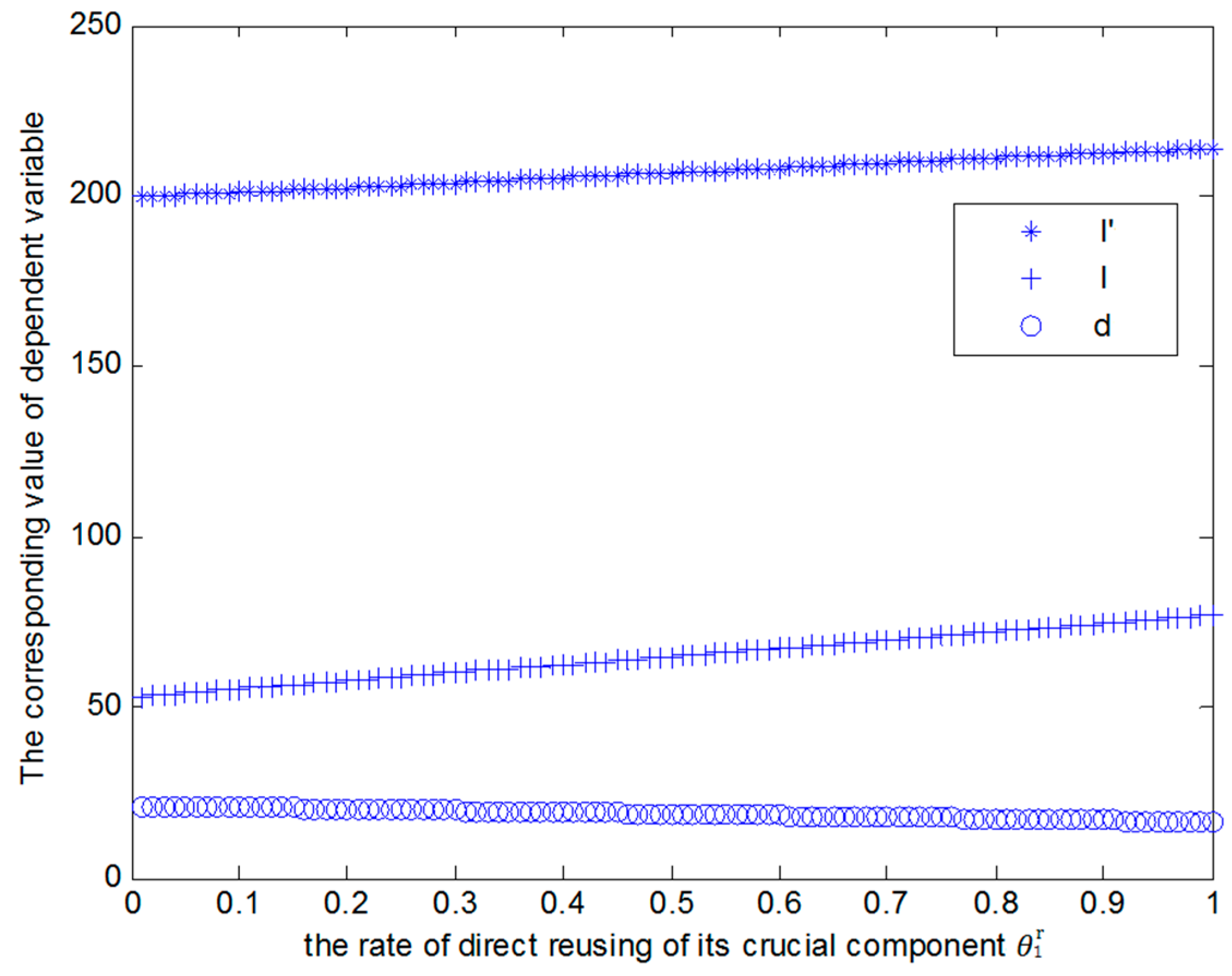
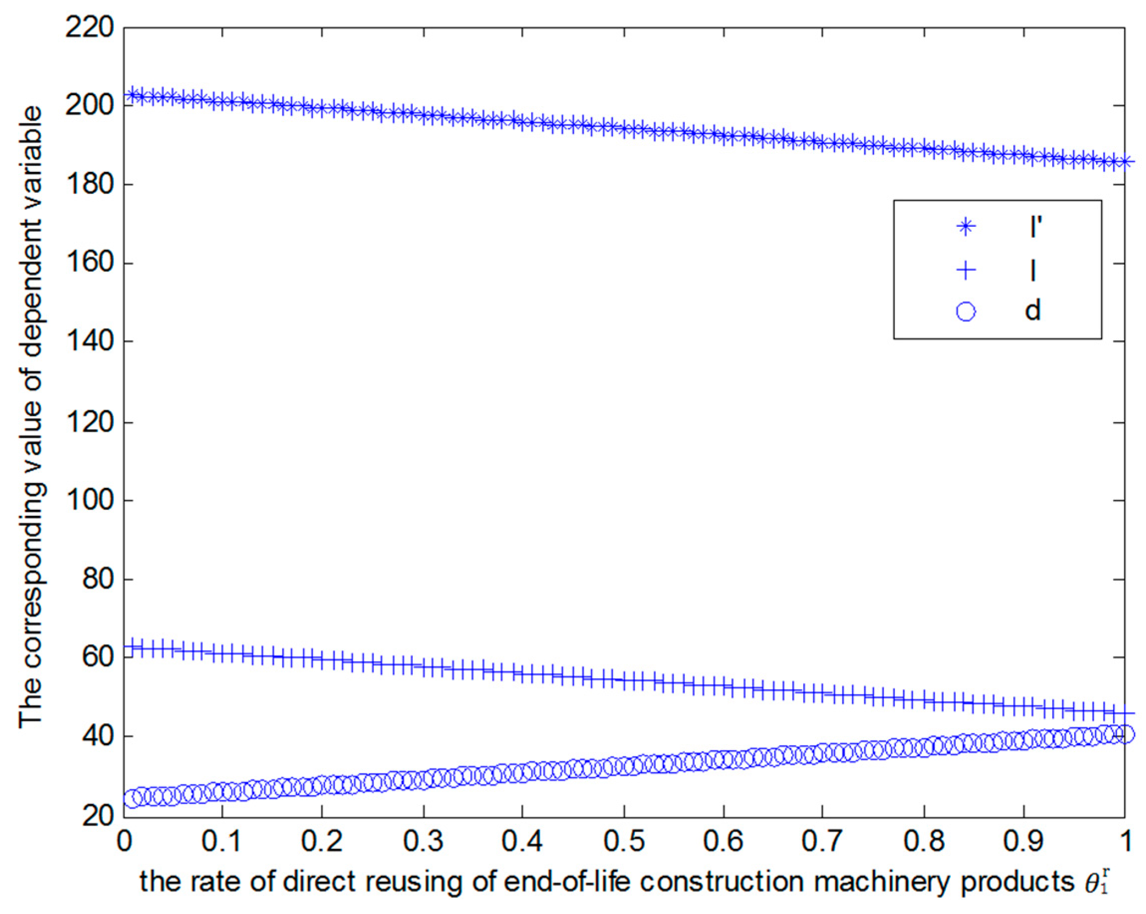
5.3. Example Analysis of the Direct Reusing Rate of EOL Product and Its Components

According to the analysis in Section 4.3, the impact of the direct reusing rate of EOL product (${\theta }_1^r$) and its components (${\theta }_2^r$) on resource benefits of unit remanufacturing product ($l$), profits and costs of unit remanufacturing product ($l^{\prime }$ and $d$) are dependent on, ${\mu }_1$, ${\epsilon }_1$, ${\phi }_2$, ${\mu }_2$, ${\epsilon }_2$, ${\phi }_3$, ${\mu }_3$ and ${\epsilon }_3$, the variation trend of $l^{\prime }$, $l$ and $d$ contains three aspects through example verification: when ${\phi }_3>\frac{{\theta }_3^r}{1-{\theta }_1^r}{\phi }_1+\frac{{\theta }_2^r}{1-{\theta }_1^r}{\phi }_2$ and ${\phi }_1<{\phi }_2$, or ${\mu }_3>\frac{{\theta }_3^r}{1-{\theta }_1^r}{\mu }_1+\frac{{\theta }_3^r}{1-{\theta }_1^r}{\mu }_2$ and ${\mu }_1<{\mu }_2$, ${\epsilon }_3<\frac{{\theta }_3^r}{1-{\theta }_1^r}{\epsilon }_1+\frac{{\theta }_3^r}{1-{\theta }_1^r}{\epsilon }_2$ and ${\epsilon }_1>{\epsilon }_2$. Then we design the example as ${\alpha }_Y^X=0.6$, ${\theta }^g=0.8$, ${\alpha }^X=0.4$, ${\theta }_1^r=0.4$, ${\theta }_2^r=0.42$, $\mathrm{a}=180$, ${\theta }^q=0.8$, $v_1^1=20$, $v_2^1=15$, $v_3^1=15$, $w_1^1=10$, $w_2^1=15$, $w_1^2=15$, $w_2^2=20$, $x_1^1=1$, $x_2^1=1.5$, $x_1^2=3$, $x_2^2=4$, $x_3^2=5$, $C_3^d=15$, $C_2^d=12$, $P^r=80$, $p_m=2$, $z=5$.

Then $\{\begin{array}{l}{l}^{\prime }\left({\theta }_1^r\right)=202.8-17.2{\theta }_1^r\\ l^{\prime }\left({\theta }_2^r\right)=199.6+14.4{\theta }_2^r\end{array}$ $\{\begin{array}{l}l\left({\theta }_1^r\right)=63-17{\theta }_1^r\\ l\left({\theta }_2^r\right)=53+24{\theta }_2^r\end{array}$ $\{\begin{array}{l}d\left({\theta }_1^r\right)=24.4+16.4{\theta }_1^r\\ d\left({\theta }_2^r\right)=21.2-4.8{\theta }_2^r\end{array}$ From the equations above the variation curve of $l^{\prime }$, $l$ and $d$ in respect of ${\theta }_1^r$ and ${\theta }_1^r$ can be obtained as Figure 7 and Figure 8 are showing:

Figure 7 and Figure 8 have shown parts of the variation history of $l^{\prime }$, $l$ and $d$ in respect of ${\theta }_1^r$ and ${\theta }_2^r$: when ${\phi }_3>\frac{{\theta }_3^r}{1-{\theta }_1^r}{\phi }_1+\frac{{\theta }_2^r}{1-{\theta }_1^r}{\phi }_2$ and ${\phi }_1<{\phi }_2$, $l^{\prime }$ decreases with the rise of ${\theta }_1^r$ but increases with the rise of ${\theta }_2^r$; when ${\mu }_3>\frac{{\theta }_3^r}{1-{\theta }_1^r}{\mu }_1+\frac{{\theta }_2^r}{1-{\theta }_1^r}{\mu }_2$ and ${\mu }_1<{\mu }_2$, $d$ decreases with the rise of ${\theta }_1^r$ but increases with the rise of $\gamma$; when ${\epsilon }_3<\frac{{\theta }_3^r}{1-{\theta }_1^r}{\epsilon }_1+\frac{{\theta }_2^r}{1-{\theta }_1^r}{\epsilon }_2$ and ${\epsilon }_1>{\epsilon }_2$, $l$ increases with the rise of ${\theta }_1^r$ while decreases with the rise of ${\theta }_2^r$.

6. Conclusions

The study in this paper concentrates on the EOL construction machinery and has made an in-depth analysis of remanufacturing processes. Then, the potential factors that affect the profits and resource benefit of remanufacturing are identified, and a resource benefits evaluation model is built up under the uncertainty of recycling price. Through this model, the recycling price and profits of remanufacturer have been obtained based on the maximization of resources benefits. Beyond all that, this paper has also explored the change regularity of resource benefits, the recycling price and profits of remanufacturer when such parameters are varying as recycling price, quality of EOL products, customer demands and direct utilization ratio of product and its components.

Conclusions drawn in this paper can be shown as follows:

(1)

If the condition whether the demands in the current period is satisfied or not is independent on previous state, then the ultimate value of customer demands satisfaction of multi-periods converges to a fixed value.

(2)

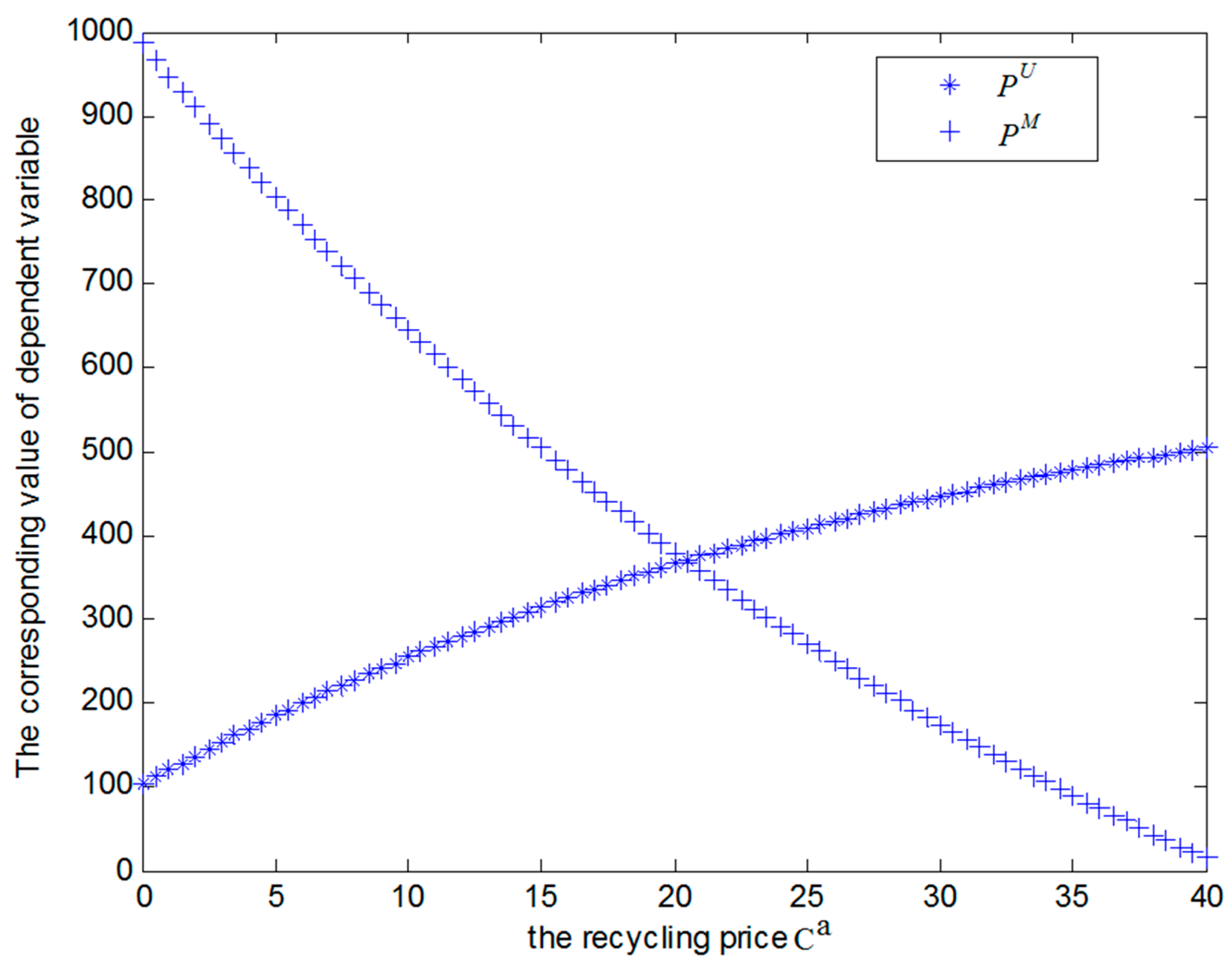
When recycling price is rising, the maximal resource benefits and the profits of remanufacturer are showing a decline trend, and the maximal resource benefits is a convex function of recycling price, the profits of remanufacturer is a concave function of recycling price. The decline rate of remanufacturer profits is higher than that of total resource benefits in remanufacturing.

(3)

There is a recycling price to make the resource benefits and the profits of remanufacturer and the value of recycling price is dependent upon the rate of the direct reusing of EOL construction machinery, the rate of the direct reusing of its crucial component and quality fluctuation coefficient.

(4)

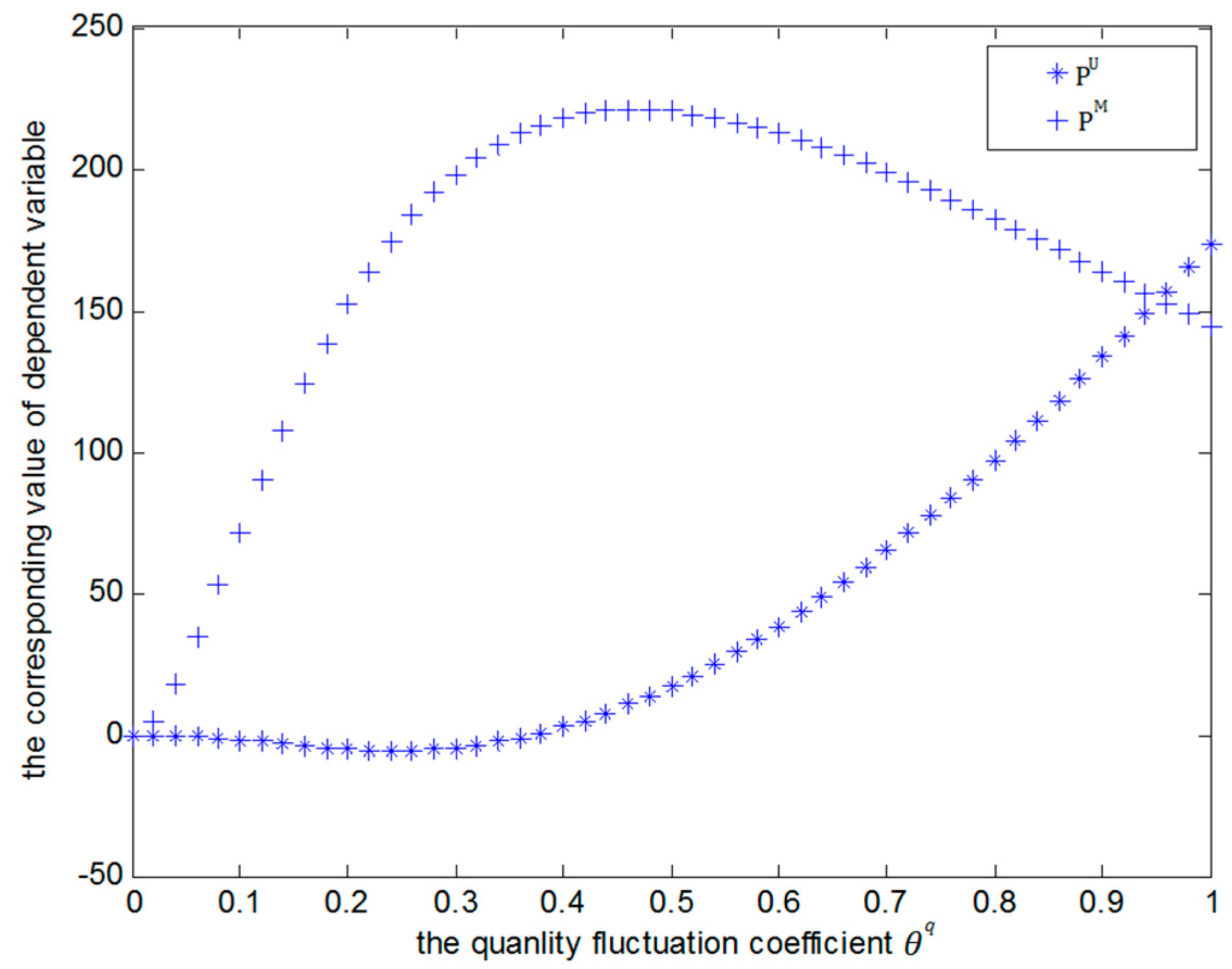
As the rise of the quality fluctuation coefficient, the profits of remanufacturer, resource benefits and the recycling price are decreasing gradually, furthermore, the decline rate of total resource benefits in remanufacturing is much higher than the recycling price and the profit of remanufacturer. However, when the quality fluctuation coefficient is approaching 1, the values of the profits of remanufacturer, the maximal resource benefits and recycling price grade into constants. Meanwhile, the optimal value of the quality fluctuation coefficient, which can make the resource benefit reach its maximum value, is related to the direct reusing rate of EOL construction machinery and the reusing rate after repairing of the crucial components. In addition, the quality fluctuation coefficient is also influenced by the value of profits of unit EOL construction machinery product and the price-elasticity index: the larger profits of unit EOL construction machinery product and the price-elasticity index are, the smaller the value of the quality fluctuation coefficient will be.

Those results can provide government and manufacturers with decision support and lead the price of EOL machinery products change within a reasonable range, such as:

(1)

When EOL products are remanufactured by the recycling price under the maximum resources benefits, the profits of remanufacturer will decrease to some extent. Therefore, while regulating the price in market, the government should also offer remanufacturer appropriate subsidies to arouse their enthusiasm.

(2)

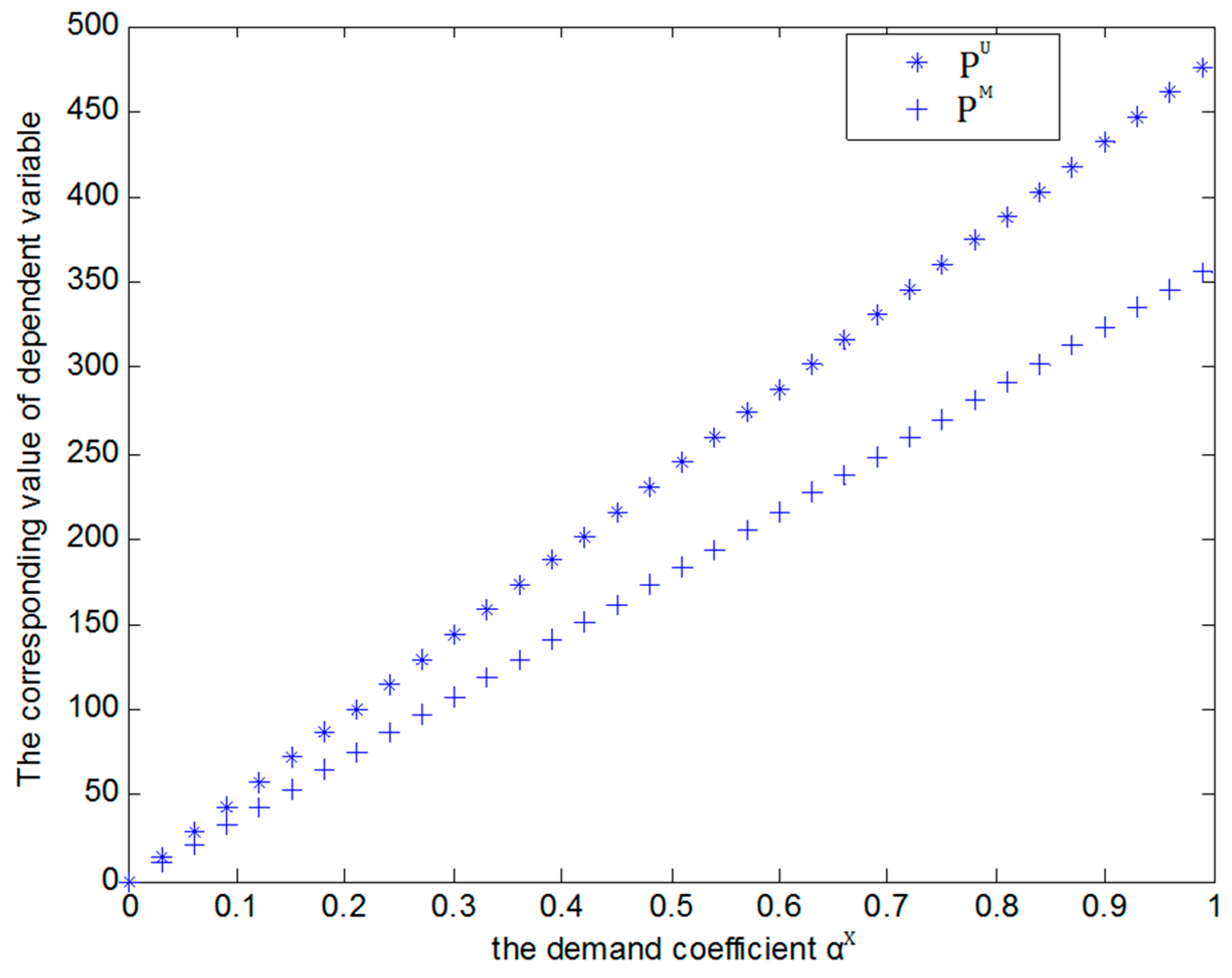
The model analysis indicates that the demand and acceptance of customers to remanufactured products present a positive correlation to resources benefits. Therefore, enterprises are required to take appropriate marketing strategy (such as advertising, public image) for improving the customer acceptance of remanufacturing products.

(3)

The recycling price can be determined by remanufacturer according to the actual value of quality fluctuation coefficient; conversely, it is also feasible to choose EOL products of better quality from recycling merchants in light of the actual recycling price.

(4)

The expression of quality fluctuation coefficient shows that the smaller the value of the quality fluctuation coefficient is, the larger the profits of remanufacturer and the price-elasticity index will be. Moreover, the value of quality fluctuation coefficient directly decided by the direct reusing rate of EOL construction machinery and its components, so when recycling the EOL construction products, remanufacturers should choose those products that their quality is comparatively low but the parts of them can be reused directly, which can ensure not only low recycling price but also larger quantity of reusable parts to increase the remanufacturing profits.

(5)

Through the analysis on uncertain parameters in this model, they can also make these uncertain factors controlled in a reasonable range, in order to coordinate between profits and resource benefits, and promote healthy development of the whole remanufacturing industry. The details of how the parameters affect the conclusions of the model and how they affect optimality and managerial decisions are shown in Appendix E.

References

1. Binshi, X.U. Remanufacture Engineering and Its Development in China. China Surf. Eng. 2010, 23, 1–6. [Google Scholar]
2. Deng, Q.; Liu, X.; Liao, H. Identifying Critical Factors in the Eco-Efficiency of Remanufacturing Based on the Fuzzy DEMATEL Method. Sustainability 2015, 7, 15527–15547. [Google Scholar] [CrossRef]
3. Xu, B. States and prospects of china characterised quality guarantee technology system for remanufactured parts. J. Mech. Eng. 2013, 49, 84. [Google Scholar] [CrossRef]
4. Yan, C. Remanufacturing and benefits analysis of construction machinery hydraulic valves. China Surf. Eng. 2013, 401–403, 2266–2270. [Google Scholar] [CrossRef]
5. Li, X.; Li, Y.; Cai, X. Remanufacturing and pricing decisions with random yield and random demand. Comput. Oper. Res. 2015, 54, 195–203. [Google Scholar] [CrossRef]
6. Ketzenberg, M.E.; Zuidwijk, A.A. Optimal Pricing, Ordering, and Return Policies for Consumer Goods. Prod. Oper. Manag. 2009, 18, 344–360. [Google Scholar] [CrossRef]
7. Guo, J.H.; Yang, L.; Li, B.L.; Ni, M. Jointed pricing decision of remanufacturing system under uncertain demand. Syst. Eng.-Theory Pract. 2013, 33, 1949–1955. [Google Scholar]
8. Meng, K.; Lou, P.; Peng, X.; Prybutok, V. An improved co-evolutionary algorithm for green manufacturing by integration of recovery option selection and disassembly planning for end-of-life products. Int. J. Prod. Res. 2016, 54, 1–27. [Google Scholar] [CrossRef]
9. Ghazalli, Z.; Murata, A. Development of an AHP-CBR evaluation system for remanufacturing: End-of-life selection strategy. Int. J. Sustain. Eng. 2011, 4, 2–15. [Google Scholar] [CrossRef]
10. Galbreth, M.R.; Blackburn, J.D. Optimal Acquisition and Sorting Policies for Remanufacturing. Prod. Oper. Manag. 2006, 15, 384–392. [Google Scholar] [CrossRef]
11. Sabharwal, S.; Garg, S. Determining cost effectiveness index of remanufacturing: A graph theoretic approach. Int. J. Prod. Econ. 2013, 144, 521–532. [Google Scholar] [CrossRef]
12. Golinska, P.; Kuebler, F. The Method for Assessment of the Sustainability Maturity in Remanufacturing Companies ☆. Procedia Cirp 2014, 15, 201–206. [Google Scholar] [CrossRef]
13. Geyer, R.; Atasu, A. The Economics of Remanufacturing Under Limited Component Durability and Finite Product Life Cycles. Manag. Sci. 2007, 53, 88–100. [Google Scholar] [CrossRef]
14. Luglietti, R.; Taisch, M.; Magalini, F.; Cassina, J.; Mascolo, J.E. Environmental and economic evaluation of end-of-life alternatives for automotive engine. In Proceedings of the 2014 International ICE Conference on Engineering, Technology and Innovation, Bali, Indonesia, 23–25 June 2014.
15. Du, Y.; Li, C. Implementing energy-saving and environmental-benign paradigm: Machine tool remanufacturing by OEMs in China. J. Clean. Prod. 2014, 66, 272–279. [Google Scholar] [CrossRef]
16. Goldey, C.L.; Kuester, E.-U.; Mummert, R.; Okrasinski, T.A.; Olson, D.; Schaeffer, W.J. Lifecycle assessment of the environmental benefits of remanufactured telecommunications product within a “green” supply chain. In Proceedings of the IEEE International Symposium on Sustainable Systems and Technology, Arlington, VA, USA, 17–19 May 2010.
17. Zahedi, H.; Mascle, C.; Baptiste, P. A quantitative evaluation model to measure the disassembly difficulty; application of the semi-destructive methods in aviation End-of-Life. Int. J. Prod. Res. 2016, 54, 3736–3748. [Google Scholar] [CrossRef]
18. Yi, P.; Huang, M.; Guo, L.; Shi, T. A retailer oriented closed-loop supply chain network design for end of life construction machinery remanufacturing. J. Clean. Prod. 2016, 124, 191–203. [Google Scholar] [CrossRef]
19. Diener, D.L.; Tillman, A.M. Scrapping steel components for recycling—Is not that good enough? Seeking improvements in automotive component end-of-life. Resour. Conserv. Recycl. 2016, 110, 48–60. [Google Scholar] [CrossRef]
20. Wolfram, P.; Wiedmann, T.; Diesendorf, M. Carbon footprint scenarios for renewable electricity in Australia. J. Clean. Prod. 2016, 124, 236–245. [Google Scholar] [CrossRef]
21. Xiong, Z.K.; Cao, J.; Liu, K.J. Study On the Quality Control Policy in the Closed-loop Supply Chain Based on the Dynamic Game Theory. Chin. J. Manag. Sci. 2007, 15, 42–50. [Google Scholar]
22. Jin, X.; Hu, S.; Ni, J.; Xiao, G. Assembly Strategies for Remanufacturing Systems With Variable Quality Returns. IEEE Trans. Autom. Sci. Eng. 2014, 4, 1–18. [Google Scholar] [CrossRef]
23. Abdulrahman, M.D.; Gunasekaran, A.; Subramanian, N. Critical barriers in implementing reverse logistics in the Chinese manufacturing sectors. Eng. Costs Prod. Econ. 2014, 147, 460–471. [Google Scholar] [CrossRef]
24. González-Torre, P.; Alvarez, M.; Sarkis, J.; Adenso-Diaz, B. Barriers to the Implementation of Environmentally Oriented Reverse Logistics: Evidence from the Automotive Industry Sector. Br. J. Manag. 2010, 21, 889–904. [Google Scholar] [CrossRef]
25. Ferrer, G.; Swaminathan, J.M. Managing new and differentiated remanufactured products. Eur. J. Oper. Res. 2010, 203, 370–379. [Google Scholar] [CrossRef] [Green Version]
26. Xiang, L.I.; Yong-Jian, L.I.; Cai, X.Q. Collection pricing decision in a remanufacturing system considering random yield and random demand. Syst. Eng. 2009, 29, 19–27. [Google Scholar]
27. Huang, M.; Yi, P.; Shi, T.; Guo, L. A modal interval based method for dynamic decision model considering uncertain quality of used products in remanufacturing. J. Intell. Manuf. 2015. [Google Scholar] [CrossRef]
28. Sutherland, J.W.; Jenkins, T.L.; Haapala, K.R. Development of a cost model and its application in determining optimal size of a diesel engine remanufacturing facility. CIRP Ann. 2010, 59, 49–52. [Google Scholar] [CrossRef]
29. Pandey, V.; Thurston, D. Variability and Component Criticality in Component Reuse and Remanufacturing Systems. J. Comput. Inf. Sci. Eng. 2007, 10, 208–216. [Google Scholar]
30. Zhang, T.; Chu, J.; Wang, X.; Liu, X.; Cui, P. Development pattern and enhancing system of automotive components remanufacturing industry in China. Resour. Conserv. Recycl. 2011, 55, 613–622. [Google Scholar] [CrossRef]
31. Sundin, E.; Hui, M.L. In what way is remanufacturing good for the environment? In Design for Innovative Value towards a Sustainable Society; Springer: Berlin, Germany, 2012; pp. 552–557. [Google Scholar]
32. Haapala, K.R.; Zhao, F.; Camelio, J.; Sutherland, J.W.; Skerlos, S.J.; Dornfeld, D.A.; Jawahir, I.S.; Clarens, A.F.; Rickli, J.L. A Review of engineering research in sustainable manufacturing. J. Manuf. Sci. Eng. 2013, 135, 599–619. [Google Scholar] [CrossRef]
33. Wu, Y.; Li, W.; Yang, P. A study of fatigue remaining useful life assessment for construction machinery part in remanufacturing. Procedia Cirp 2015, 29, 758–763. [Google Scholar] [CrossRef]
34. Xia, X.; Govindan, K.; Zhu, Q. Analyzing internal barriers for automotive parts remanufacturers in China using grey-DEMATEL approach. J. Clean. Prod. 2015, 87, 811–825. [Google Scholar] [CrossRef]
35. Zhu, Q.; Sarkis, J.; Lai, K.H. Supply chain-based barriers for truck-engine remanufacturing in China. Transp. Res. Part E Logist. Transp. Rev. 2015, 68, 103–117. [Google Scholar] [CrossRef]
36. Teunter, R.H.; Flapper, S.D.P. Optimal core acquisition and remanufacturing policies under uncertain core quality fractions. Eur. J. Oper. Res. 2011, 210, 241–248. [Google Scholar] [CrossRef]
Figure 1. The remanufacturing processes flowchart of EOL construction machinery.
Sustainability 09 00256 g001
Figure 2. Uncertainty factors existing in the process of recycling and remanufacturing processes.
Sustainability 09 00256 g002
Figure 3. Three cases of direct reusing rate of EOL products.
Sustainability 09 00256 g003
Figure 4. The impact of recycling price on P U and P M .
Sustainability 09 00256 g004
Figure 5. The impact of α X on P U and P 1 M .
Sustainability 09 00256 g005
Figure 6. The impact of quality fluctuation coefficient θ q on P U and P 1 M .
Sustainability 09 00256 g006
Figure 7. Impact of θ 1 r on l, l’ and d.
Sustainability 09 00256 g007
Figure 8. Impact of θ 2 r on l, l’ and d.
Sustainability 09 00256 g008