1. Introduction
Probabilistic information about the future values of the spot electricity price is very valuable for the operational planning and trading of conventional and renewable energy generation companies, as well as to implement demand response products [
1] or foster the participation of large electrical energy consumers in the wholesale electricity market [
2]. Moreover, advanced short-term risk hedging strategies (see [
3] for the mathematical formulations) require probabilistic forecasts for day-ahead and intraday market sessions.
Probabilistic forecasting is defined as a conditional estimation (i.e., conditioned by a set of explanatory variables) of a probability distribution that is likely to contain the real value of the electricity price. In this paper, the uncertainty forecast is represented by a set of conditional quantiles. The time horizon is short-term forecasting, i.e., day-ahead and intraday markets. For the mid-term time horizon, recent advances with an hourly time resolution and probabilistic forecasts can be found in [
4,
5].
Early works in price forecasting were mainly focused on producing accurate point (or deterministic) forecasts represented by the conditional expectation of the future price value. A comprehensive literature review can be found in [
6]. Szkuta et al. applied artificial neural networks (ANN) for day-ahead price forecasting using as inputs lagged variables of power reserves, potential demand, marginal price and calendar variables [
7]. Conejo et al. decomposed the historical price series, using the wavelet transform in a set of four constitutive series and, in a second phase, ARIMA models were fitted to each constitutive time series in order to produce day-ahead price forecasts [
8]. A similar approach was followed by Shafie-khah et al. that combines wavelet transform, ARIMA and radial basis function ANN [
9]. Nogales and Conejo proposed transfer function models that outperformed ARIMA and ANN [
10]. Lora et al. proposed a weighted nearest neighbors methodology that outperforms ANN, neuro-fuzzy system and GARCH models [
11].
For markets with locational marginal prices (LMP), like the U.S.A., Kekatos et al. formulate the day-ahead price forecasting problem as a low-rank kernel learning problem and account for the congestion mechanisms causing the LMP variations [
12]. Li et al. proposed a forecasting system that integrates fuzzy inference, linear regressive model and market power metrics [
13]. These models used the following inputs: calendar variables, past LMP and zonal loads of previous intervals.
Current research is focused in probabilistic forecasting of market prices. Zhao et al. introduced a heteroscedastic variance equation for the support vector machine algorithm in order to generate forecast intervals for the price variable [
14]. The probabilistic forecasts from this method consisted of mean and variance, which is only suitable for parametric representations like the Gaussian distribution. The Gaussian assumption is also followed by Wan et al., which proposed extreme learning machines (ELM) combined with a maximum likelihood estimation of the noise variance [
15]. Dudek applied ANN to day-ahead point forecasting and probabilistic forecasts were generated by assuming: (i) Gaussian distribution for forecast errors and that (ii) forecast errors on the training and test sets have the same distribution [
16].
It was shown in [
17] that the conditional price distribution is non-Gaussian. For instance, renewable energy sources (RES) generation level has an impact in the shape of the conditional probability distribution [
17,
18]. Therefore, methods that avoid the Gaussian assumption for the conditional probability distribution are required. Chen et al. also explored ELM, but combined with bootstrapping to construct forecast intervals represented by non-parametric percentiles [
19]. Juban et al. combine an L2 regularized linear quantile regression with radial basis functions for non-linear feature transformations [
20]. The input data were zonal and system loads, lagged prices, standard deviation of the price during the previous day, maximum price variation from the previous day and calendar variables. Nowotarski and Weron proposed the method Quantile Regression Averaging (QRA) that applies linear quantile regression to a pool of individual point forecasts and showed that it outperformed the best individual model [
21]. QRA was extended by Maciejowsk et al. by using principal component analysis for selecting a subset of individual forecasts [
22]. Gaillard et al. won the price forecast track of the Global Energy Forecasting Competition 2014 (GEFCom2014) [
23] by combining linear quantile regression and linear additive models to generate probabilistic price forecasts [
24]. Moreover, the QRA method was modified to have time varying weights and combined 13 different individual models. Maciejowska and Nowotarski applied three data filtering methods to historical price data [
25]: day-type filtering; similar load profile filtering; expected bias filtering. Then, an autoregressive model with exogenous variables (ARX) was used to generate point forecasts and probabilistic forecasts were produced with linear quantile regression that combines expected price levels generated by multiple models.
A common characteristic of all these works is that only lagged values of price and load, together with calendar variables, are used as explanatory variables. However, other variables might influence the price level and uncertainty. For instance, statistical analysis showed that RES generation level has a significant impact in the spot price of countries with high RES integration levels like Germany [
26], Denmark [
27] and Portugal [
18]. Other variables like natural gas prices volatility [
28] or the share of hydropower in each market session (or neighboring country) [
29] also exhibit a strong influence in the spot price. A point forecasting method that included the impact of forecasted system load and wind power generation was proposed by Jónsson et al., which combined local linear models to capture time varying and non-linear relations with time series models (i.e., ARMA and Holt–Winters) to account for autocorrelation of the model’s residuals [
30]. This method was generalized in [
31] for probabilistic forecasting by proposing a time-adaptive quantile regression, which outperformed parametric Gaussian models. Monteiro et al. conducted an exploratory analysis of a set of explanatory variables in the Iberian Electricity Market (MIBEL), using ANN for the day-ahead point forecast [
32]. The analysis showed that forecasted wind speed and the price in the previous day are the most relevant variables, although other variables like hydropower and nuclear generation levels from past days give explanatory information for price forecasting. A similar analysis was conducted for the six intraday markets in MIBEL and the results showed that the best variables were the hourly prices of the daily session and previous intraday sessions, as well as calendar variables [
33]. Automatic selection algorithms can be applied to select the best set of variables [
34].
In this context, the present paper provides the following original contributions:
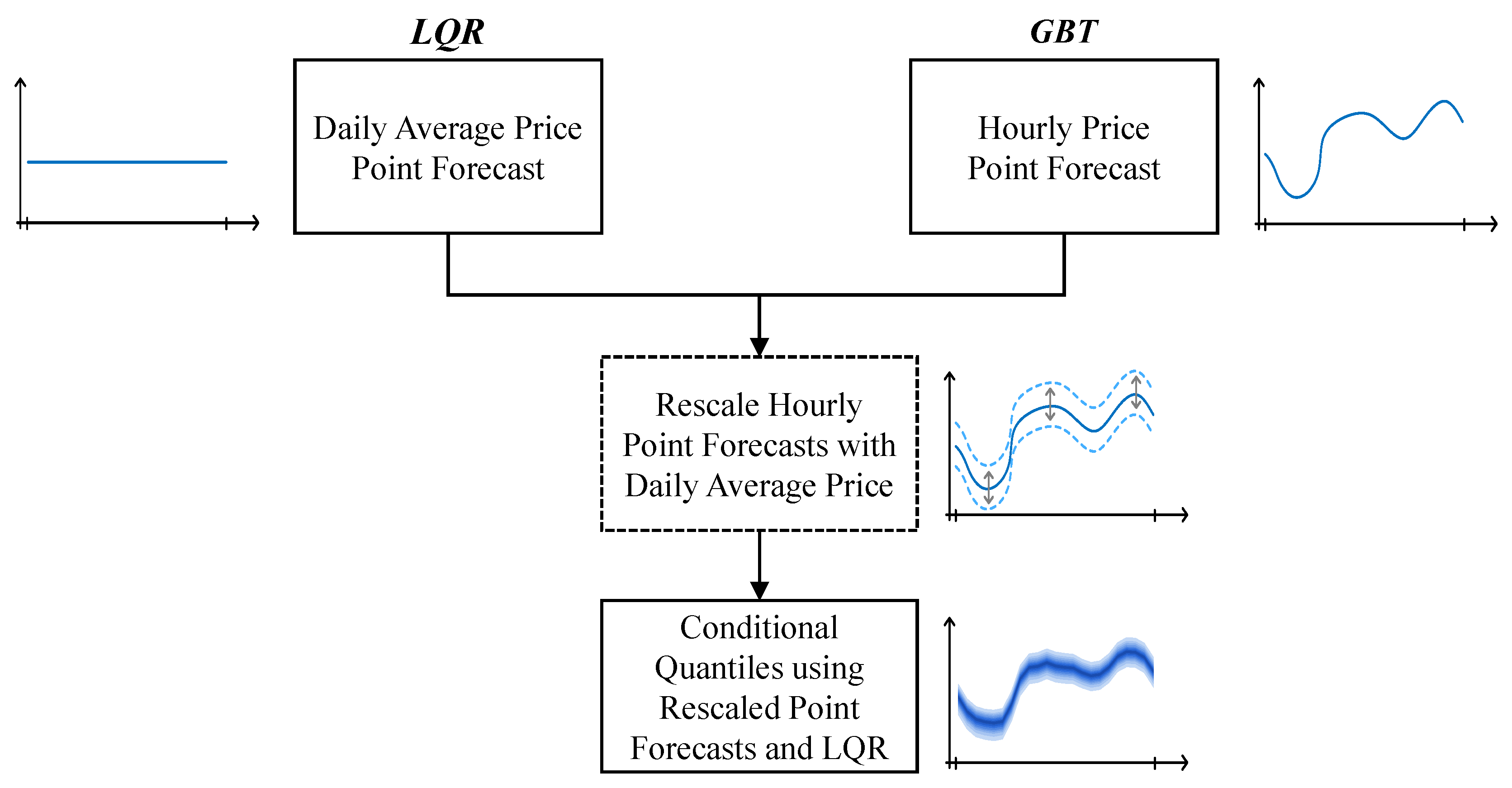
Explores price information from the futures market to improve the point and probabilistic forecasting skill of day-ahead and intraday wholesale prices. With this publicly available information, an accurate forecast for the daily average price is generated and used to rescale the point forecast generated by a gradient boosting tree model, which is later used to feed a linear quantile regression that produces conditional quantile forecasts;
Applies probabilistic forecasting techniques to both day-ahead and intraday markets, which contrasts with the work in [
32,
33] that only proposed point forecast models.
In summary, this work goes beyond the choice of the statistical model since the main focus is the selection of explanatory variables and post-processing of forecasts by exploiting the forecasted daily average price and settlement price of futures contract.
The case study is the MIBEL (Portugal and Spain) market, characterized by high shares of renewable energy (solar, wind, hydropower), and all the market and forecast data (wind, solar, load, etc.) is publicly available. The forecast results were obtained by mimicking the operation of a real forecast system, i.e., only the data available up to the market session horizon was used to generate point and probabilistic forecasts.
The remainder of the paper is organized as follows: the Iberian electricity market structure and publicly available data is described in
Section 2;
Section 3 presents the point and probabilistic price forecasting methodology applied to the day-ahead and intraday market sessions; numerical results, analysis of the different variables and methods are presented in
Section 4; finally, the main conclusions of the work are given in
Section 5.
4. Results and Discussion
4.1. Simulation of the Operational Forecast Scenario
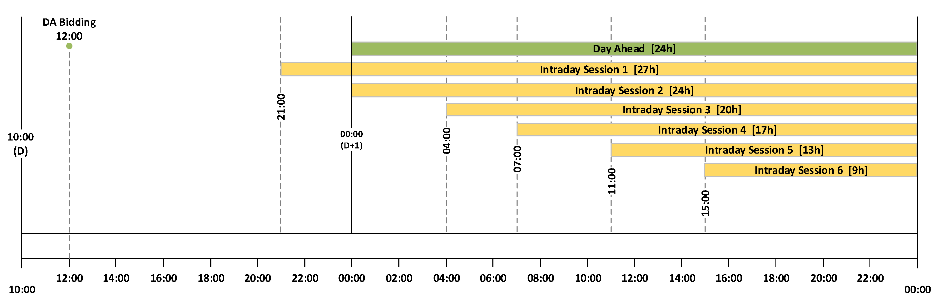
Short-term price forecasts are only relevant if generated prior to the session gate closure. Considering the timeline presented in
Section 2.1 for the DA and ID sessions, it is important to underline that the methodology presented in this paper replicates an operational forecast scenario where the data extraction and forecasts computation stages are conditioned to the information publicly available prior to market closure, guaranteeing that forecasted prices can be used by market agents in their decision-making processes.
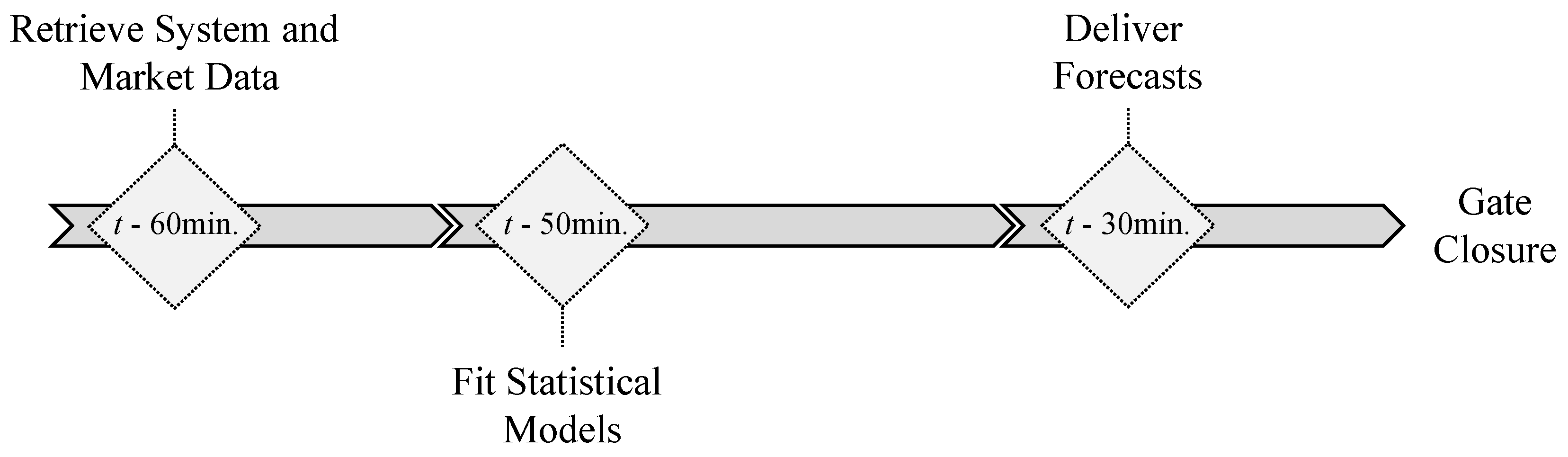
Figure 5 depicts the temporal framework of each forecast run. Assuming
t as market sessions gate closure (see
Figure 1), each forecast run is organized in three distinct phases: (i) retrieve system and market data; (ii) statistical model’s fitting; (iii) deliver forecasts.
Accordingly, all the necessary data to be used by the forecasting models is retrieved 60 min prior to gate closure ( min). Then, a model’s fitting is executed. Finally the forecasts are delivered 30 min before market gate closure ( min).
This sequence of events is repeated every day for each market session, guaranteeing that the most recent data is incorporated into the dataset used to fit the forecasting models. In each day, the training dataset used to fit the forecasting models comprises all the Iberian system data from 12 June 2015 until the forecasts launch time.
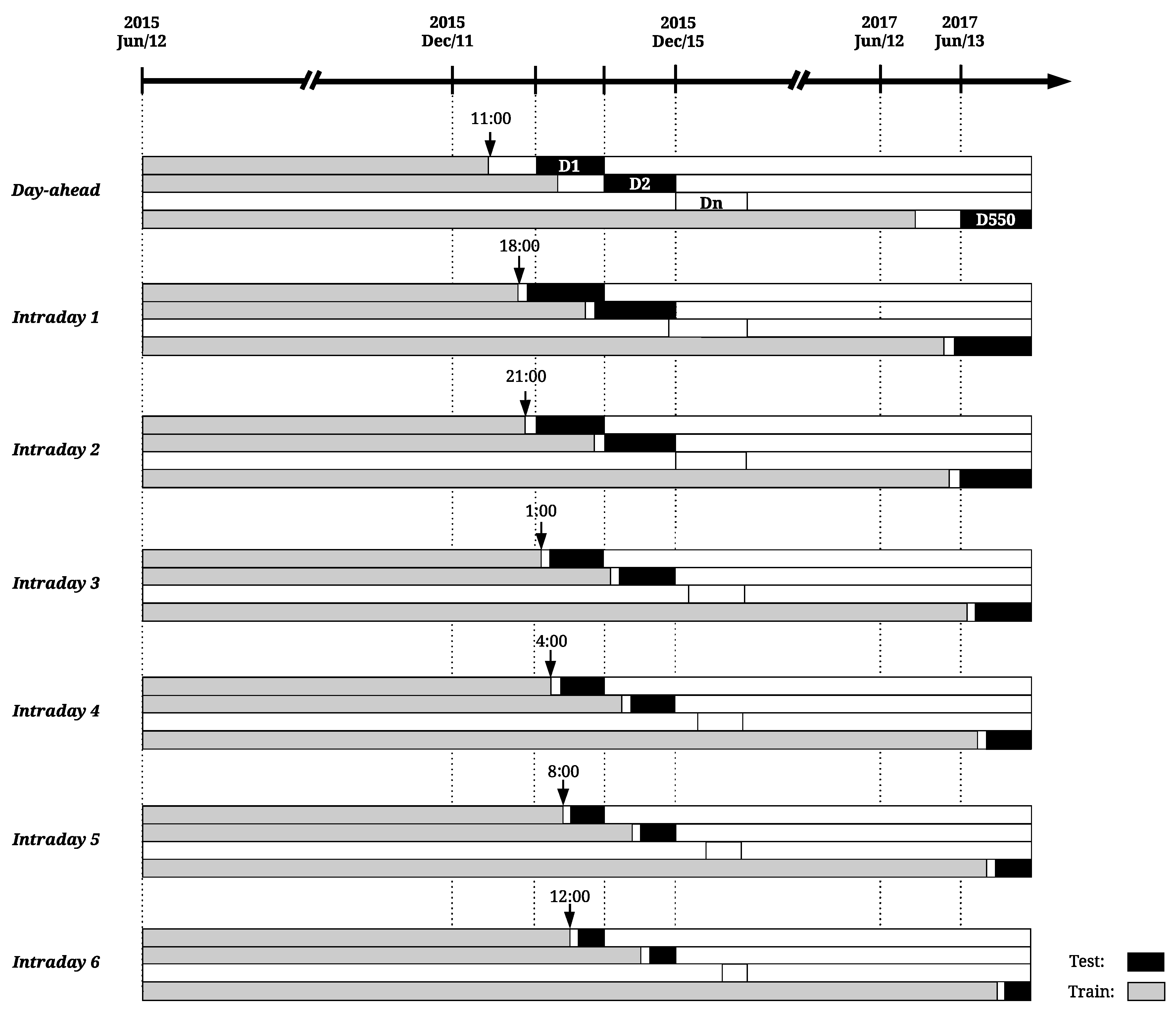
Considering the aforementioned temporal framework, a rolling window approach is here used to test each model performance along the available historical data. This test methodology is illustrated in
Figure 6, where gray colored bars represent the training data gathered from 12 June 2015 until 50 min before session gate closure (see
Figure 5) and black bars the test data of each rolling window iteration or, in other words, each day-ahead or intraday session programming period.
In the first iteration of the rolling window process, the models are fitted with six months of data (June–December 2015) and the forecasts are generated for 12 December 2015 (day
D1 of
Figure 6). This process is repeated until 13 June 2017 (day
D550 of
Figure 6), making a total of 550 iterations (or number of days in the test sample).
For DA and ID2 market sessions, the forecasts are computed at the present day (D) for the intervals 1 to 24 of day ahead (). It is important to stress that the start of the datasets used for fitting is maintained through all the validation process, forecasting models are trained in a daily basis and the size of train dataset increases in each iteration, accommodating recent system and market data.
4.2. Forecasting Skill Scores
The accuracy of point forecasts (i.e., quantile 50% in this work) was evaluated by the root mean square error (RMSE), the mean absolute error (MAE), and the mean absolute percentage error (MAPE). On the later, all the absolute percentage values above 100% were removed to exclude a small subset of cases with abnormally high percentage error due to price values close to zero, which introduced extreme and unrealistic penalties in the MAPE calculation.
The quality of probabilistic forecasts was evaluated with the following metrics: calibration, sharpness and continuous ranked probability score (CRPS).
Empirical probabilities (or long-run quantile proportions) should asymptotically approach the nominal (or subjective) probabilities. The calibration metric is used to assess this important property [
49]. This difference between empirical and nominal probabilities can be denominated as bias
of the probabilistic forecasts and is usually calculated for each quantile nominal proportion
, as follows:
for a given horizon
, where
is the indicator function evaluating if the actual price
lies below the quantile forecast
, over the evaluation set
.
Sharpness quantifies the uncertainty of the probabilistic forecasts [
49], which numerically corresponds to compute the average interval size between two symmetric quantiles (e.g.,
and
with
) as follows:
with nominal coverage rate
and horizon
.
Sharpness and calibration are intuitive properties, but can only be exploited in a diagnostic mode. On the other hand, CRPS is an unique skill score that provides the entire amount of information about a given method’s performance and encompasses information about calibration and sharpness of probabilistic forecasts. The CRPS metric was adapted to evaluate quantile forecasts (for more details see [
50]) as follows:
where
is quantile loss function defined in Equation (
3),
the actual observed price at horizon
and
the quantile
price forecast. The CRPS is given as a percentage of the maximum price
180.3 €/MWh.
Each of these metrics were calculated considering all the forecasts generated between 12 December 2015 and 13 June 2017.
4.3. Numerical Results: Day-Ahead Market
When working with datasets composed by a large number of explanatory variables, it is appropriate to apply domain knowledge combined with proper feature selection methodologies to remove unnecessary or redundant information that might decrease the performance of forecasting models.
Different feature exploration techniques can be used to narrow a large number of variables into a smaller subset that retains the most representative information. The feature evaluation methodology described in this work comprises three distinct phases. Firstly, the individual importance of every system variable to the forecasting skill is examined. Secondly, the cross-effects between variables are examined. Finally, a subset of explanatory variables capable of producing high quality hourly price forecasts is presented and the importance of the rescaling framework, described in
Section 3.1, is evaluated.
Given the extent of information available in this work, each variable is referred in the following subsections accordingly to the nomenclature presented in
Table 2.
4.3.1. Analysis of Individual Variables Effect
A preliminary analysis conducted with the full set of explanatory variables concluded that calendar variables and lagged wholesale electricity price need to be included in all models since it substantially improved the point and probabilistic forecasting skill. Therefore, a base model exclusively composed by these variables (B = {CH, CWd, CM, P}) was defined to compare and assess the importance of the remaining variables.
Table 4 summarizes the impact of each variable on point and probabilistic forecasts. The models are presented in descending order according to the MAE improvements on the aforementioned base model (B). The improvement over the base model is presented inside brackets.
By examining
Table 4, four significant improvements on point and probabilistic forecasts are observed regarding the inclusion of daily price of futures contract (FP
OMIP), wind power penetration (FW
Pen), wind power generation (FW) and residual system load (FL
Res) forecasts. Each of these variables contains information that improves a base model exclusively constituted by calendar data and past (or lagged) prices.
Comparing the improvement related to the inclusion of wind power generation and penetration, it is verifiable that the latter contributes significantly more to point and probabilistic forecast quality, providing an additional improvement of 1.22%, 2.14%, 0.43% and 1.08% on MAE, RMSE, MAPE and CRPS respectively. The remaining variables, when included separately in the base model, showed either residual or negative improvement in each score.
It is important to underline that this analysis only considers the relation effects between calendar variables, lagged prices and each new variable. Such evaluation provides significant knowledge about the importance of each variable when added alone to the forecast model and enables the creation of simple models with a small subset of information.
4.3.2. Analysis of Variables Cross-Effects
After the identification of the variables with high individual impact on the forecasting skill, it is important to assess if these have complementary or redundant information when included simultaneously in the forecasting model. In some cases, due to cross-effects between variables learned by the statistical model, some variables that led to low improvement, when individually included in the base model (see
Section 4.3.1), can improve the price forecast skill in specific events if combined with other variables in the model.
In this subsection, the cross-effects impact of the variables set is evaluated. For this purpose, a forward selection process is presented. It involves the definition of a base model to which new variables are progressively added, according to its individual importance to the forecasting skill (defined in
Section 4.3.1 Table 4). In each iteration of this process, the importance of every combination of inputs to the forecast skill is evaluated by computing the relative improvement over the base model.
Table 5 presents every combination of variables tested in this selection process. Analogously to the previous section, M
base represents the base model, composed by calendar variables and lagged prices. Gray colored cells mark the new feature included in each iteration.
In a final stage, the redundant information contained in model M21 is removed by an exploration process that tests different combinations between the 22 explanatory variables. Considering that 22 system variables are available (calendar variables remained constant thorough all tests), a total of 4,194,303 () possible combinations should be considered. However, performing such number of combinations would result in an extensive and unfeasible evaluation process. Instead, an analysis of distinct combinations of variables combined with a sensibility analysis of each variable importance resulted in a reliable subset of variables that maximized the performance of point and probabilistic models, represented by Mfinal.
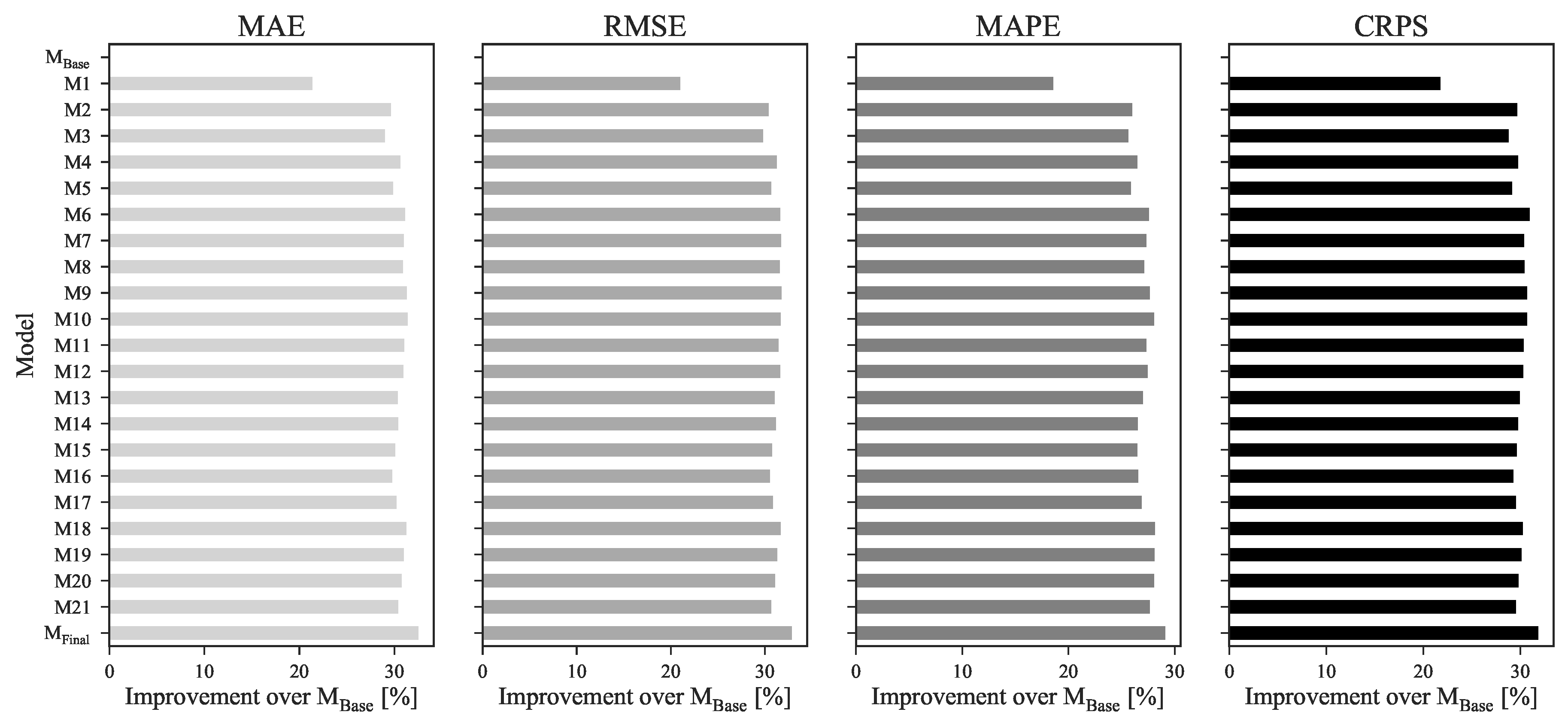
Figure 7 depicts the improvement of each model presented in
Table 5 over the base model (M
base).
A comparison between models M1 and M2 of
Figure 7 reveals that, by adding wind power penetration forecasts on top of future energy contracts settlements prices, it is possible to obtain an 10.54%, 11.93%, 9.13% and 10.12% improvement on MAE, RMSE, MAPE and CRPS scores, respectively. These two variables, besides demonstrating high importance to the forecasting skill when individually included in the forecast model, also have complementary information and increase the precision and robustness of the model while decreasing its uncertainty and point forecast errors.
For the remaining variables, the improvements are significantly less noticeable. Variables such as wind power and residual load forecasts, which led to high improvements when individually included in the base model (see
Section 4.3.1), showed some redundancy when included in a more complex model composed by the variables FP
OMIP and FW
Pen.
In contrast, by observing the higher improvements of models M6, M9, M10 and M18 on every metric, it is possible to verify that variables such as solar thermal and PV power, hydro power generation and hydro reservoir capacity, when combined with a predefined subset of other explanatory variables, contribute to increase the forecasting skill. It is important to underline that these variables showed a negative impact on the forecasting skill when added separately to the base model (see
Table 4). However, due to cross effects between all model’s variables, the introduction of these variables improved the overall accuracy.
With that being said, model Mfinal presents the best subset of explanatory variables for day-ahead market forecast. By cleaning the redundant information it was possible to reduce the number of explanatory variables from 25 to 11 while keeping the most insightful information and maximizing the predictive performance of the forecasting model. Variables such as residual load or wind power generation that demonstrated a great improvement on forecast quality when individually added to a base model, were discarded in detriment of system load and wind power penetration forecasts as they complemented significantly better the information provided by the remaining inputs. The improvements of a model trained with this final batch of explanatory variables over the base model were 32.54%, 32.87%, 29.08% and 31.85% on MAE, RMSE, MAPE and CRPS scores.
After finding the best set of explanatory variables, it was only possible to enhance the forecasting skill by rescaling the forecasts with the methodology described in
Section 3.1.3.
4.3.3. Benefits from Rescaling Day-Ahead Price Forecasts
This subsection presents a detailed comparison between the hourly forecasts obtained using the model analyzed in the previous Section (M
final) and the forecasts obtained after forcing the daily average to be equal to the forecasted daily average price (see
Section 3.1.3).
Table 6 shows the results of this comparison in terms of MAE, RMSE, MAPE and CRPS.
Just by applying the rescaling procedure to the obtained hourly forecasts (Mrescaled) and comparing with Mfinal, an improvement of more than 10% was achieved when looking to both MAE and RMSE metrics. Furthermore, it also significantly improved the MAPE (4%) and CRPS (8.8%).
When applying the LQR to the rescaled point forecasts to produce quantiles forecasts, two explanatory variables were tested: system load forecasts (FL) and wind power penetration forecasts (FWPen). By adding these two variables it was possible to decrease the MAE/RMSE by 0.13%/0.17% and 0.98%/1.17% respectively. Moreover, a positive impact in uncertainty forecast was also verified since an improvement of more than 4% was obtained in CRPS.
With the best model (Mrescaled, {FL, FWPen}), the MAE was fixed in 3.03 €/MWh, the RMSE in 4.04 €/MWh, the MAPE in 8.54% and the CRPS in 1.22%.
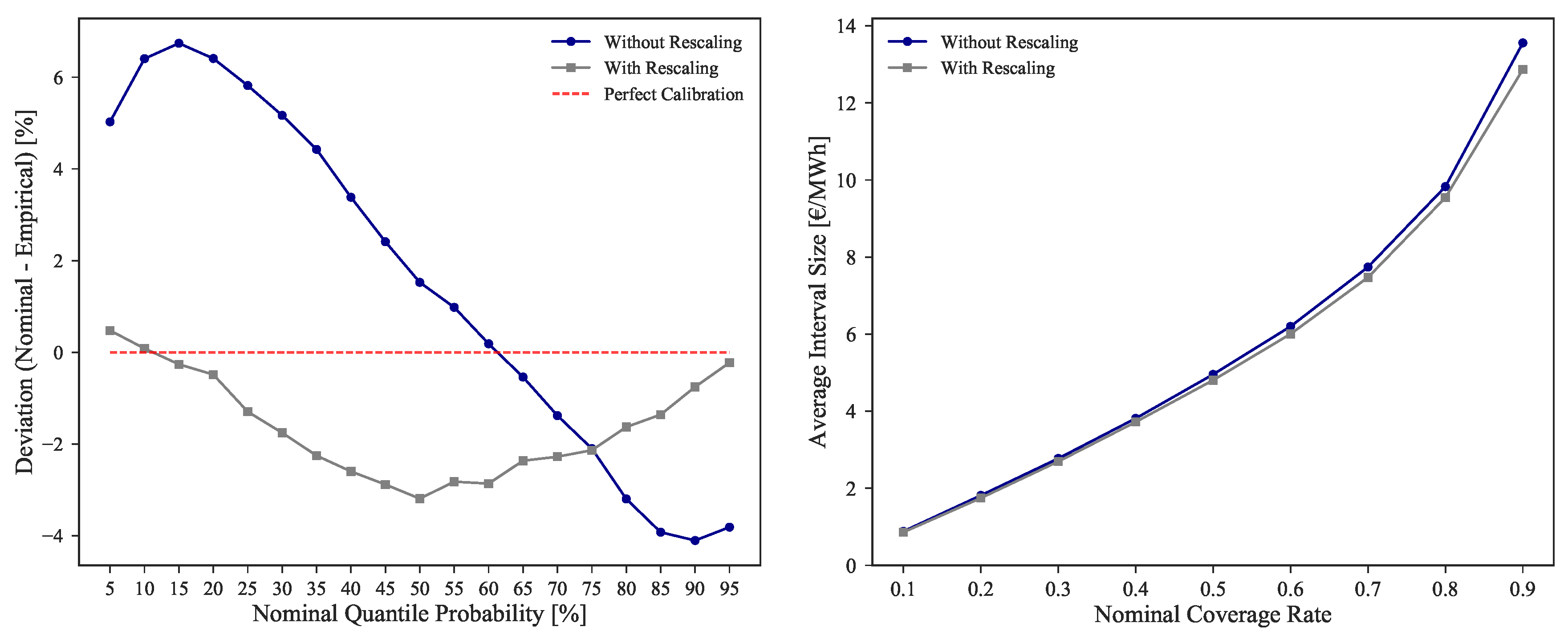
Additionally to the CRPS improvement, the calibration and sharpness were also improved.
Figure 8 shows the comparison between M
final and M
rescaled, {FL, FWPen} for these two metrics. While a minor improvement is noted on the sharpness of forecasts, in the case of calibration it is possible to observe an absolute improvement of 53.26%, more notorious in the lower and higher quantiles.
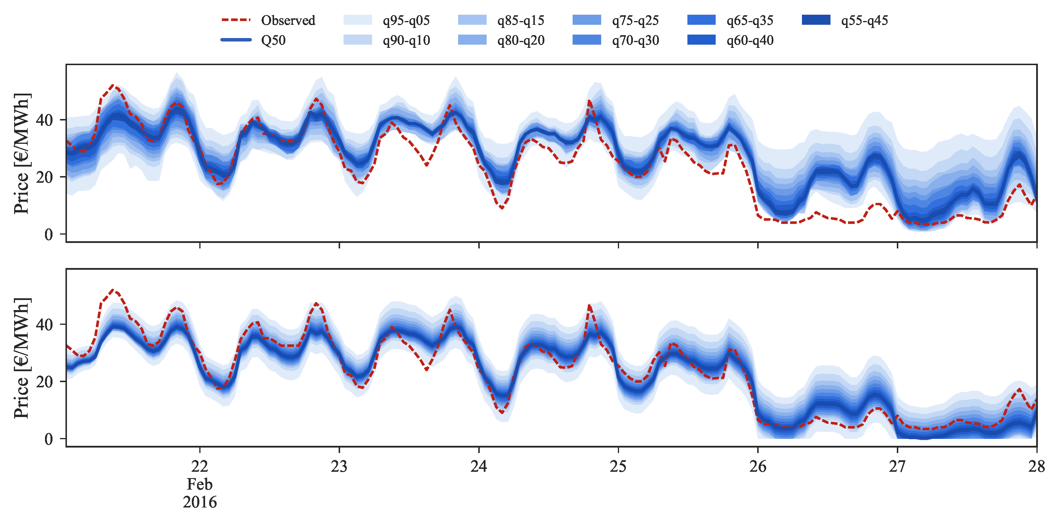
Figure 9,
Figure 10 and
Figure 11 depict a visual comparison between the forecasts before (top) and after (bottom) the application of the rescaling process. Each set of figures illustrates three distinct price regimes: low, medium and high prices.
Starting by the low prices regime, illustrated by
Figure 9 for the period between 22 and 28 February 2016, it is easily observable on the bottom side the improvement provided by the rescaling process.
In the last two days, where the observed market price reached values close to zero, the original forecasts were unable to capture the observed price curve. By applying the rescaling, the 50% quantile is now closer to the observed values and the uncertainty band (or set of forecast intervals) encompasses the observed price curve. Moreover, the sharpness of probabilistic forecasts was also drastically increased.
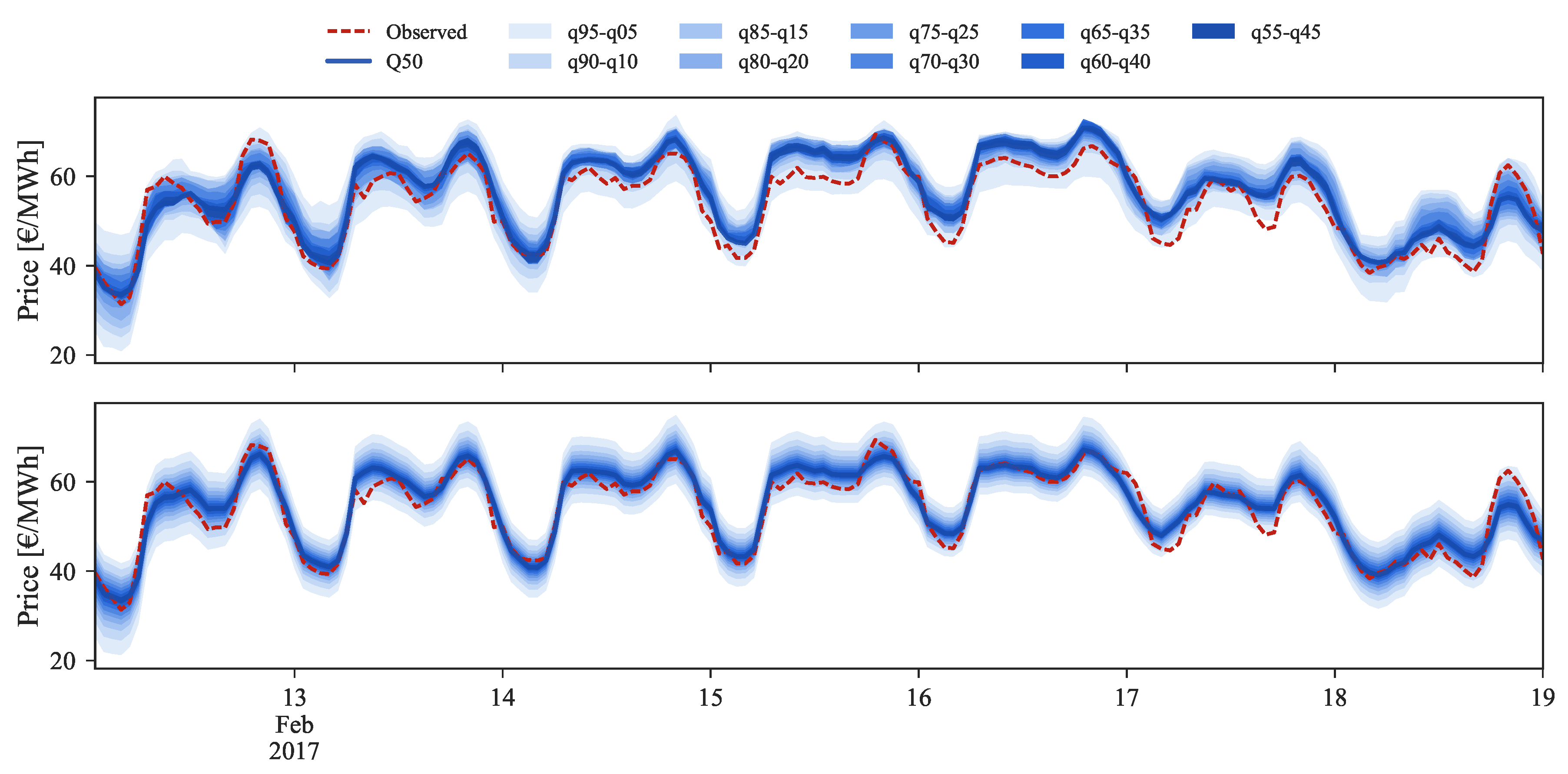
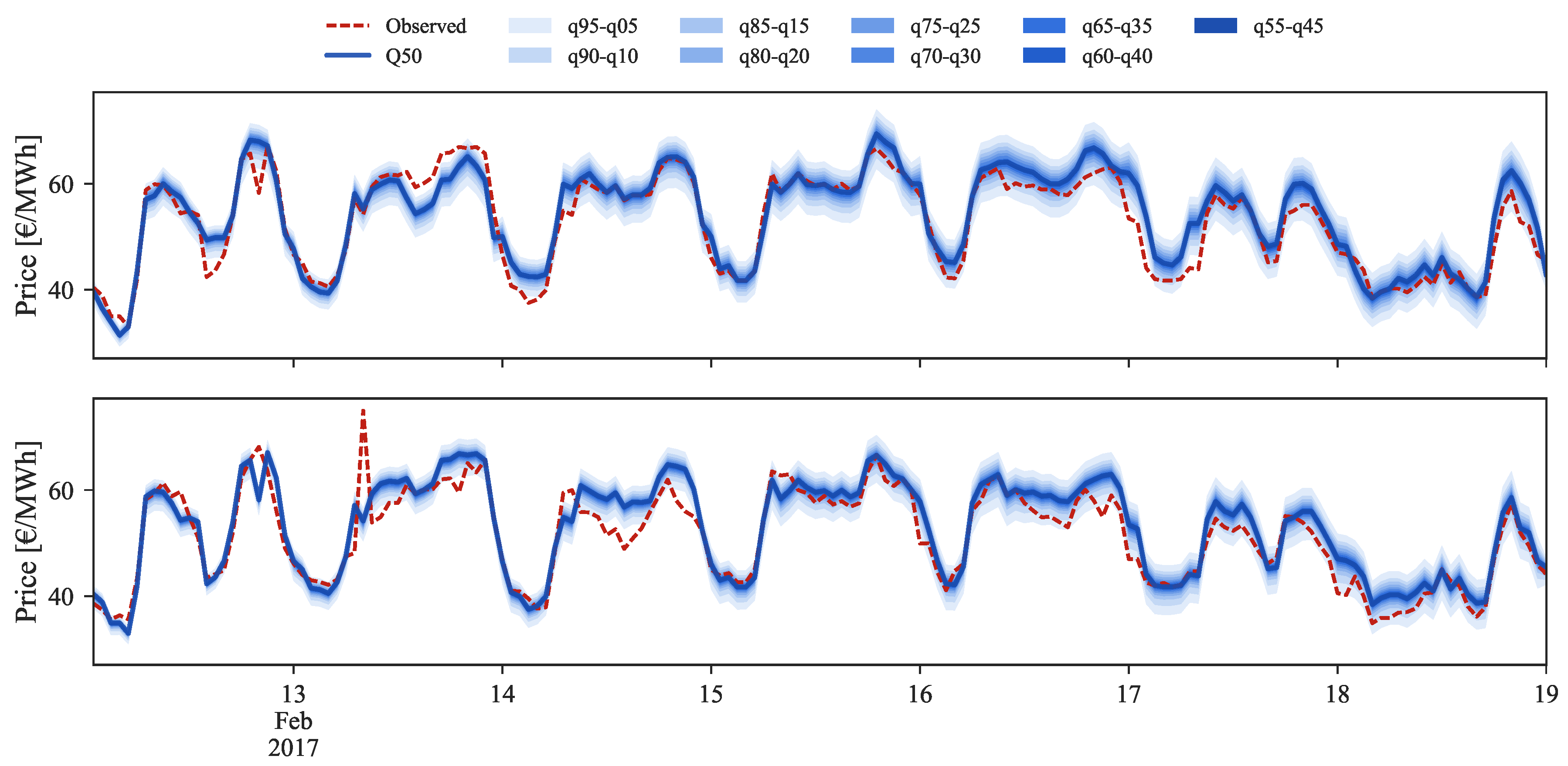
In the medium price regime (
Figure 10) for the period between 13 and 19 February 2017, the quantiles distribution is well modeled and periods in which the observed price falls outside the 5% and 95% quantiles are not verified. However, the conditional median (i.e.,
) often shows a bias with respect to the observed value. After rescaling, this bias disappears and an improvement in the probabilistic forecast sharpness is also observed.
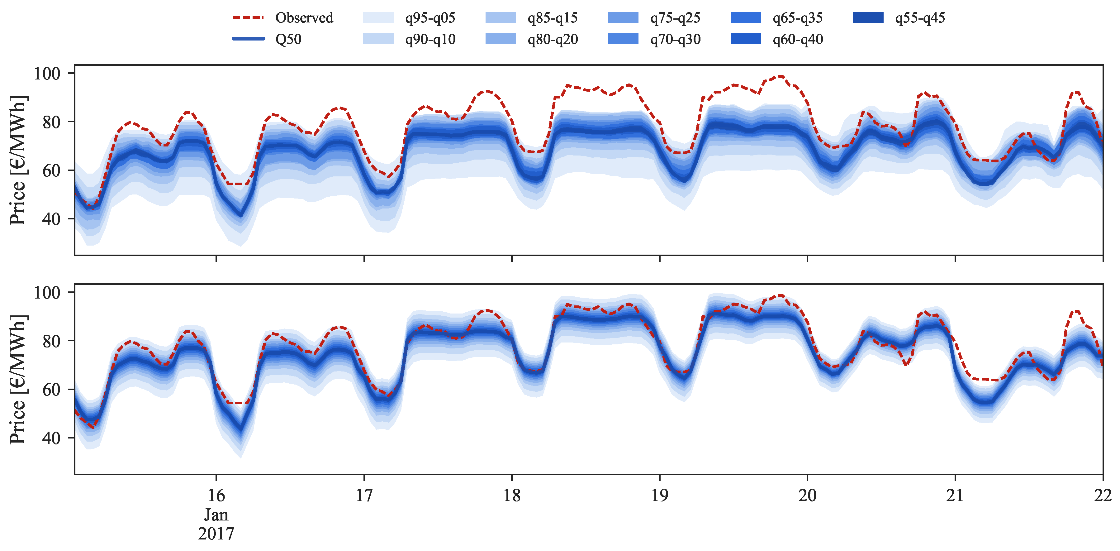
Figure 11 depicts the forecasts for the high price regime for the period between 16 and 22 January 2017.
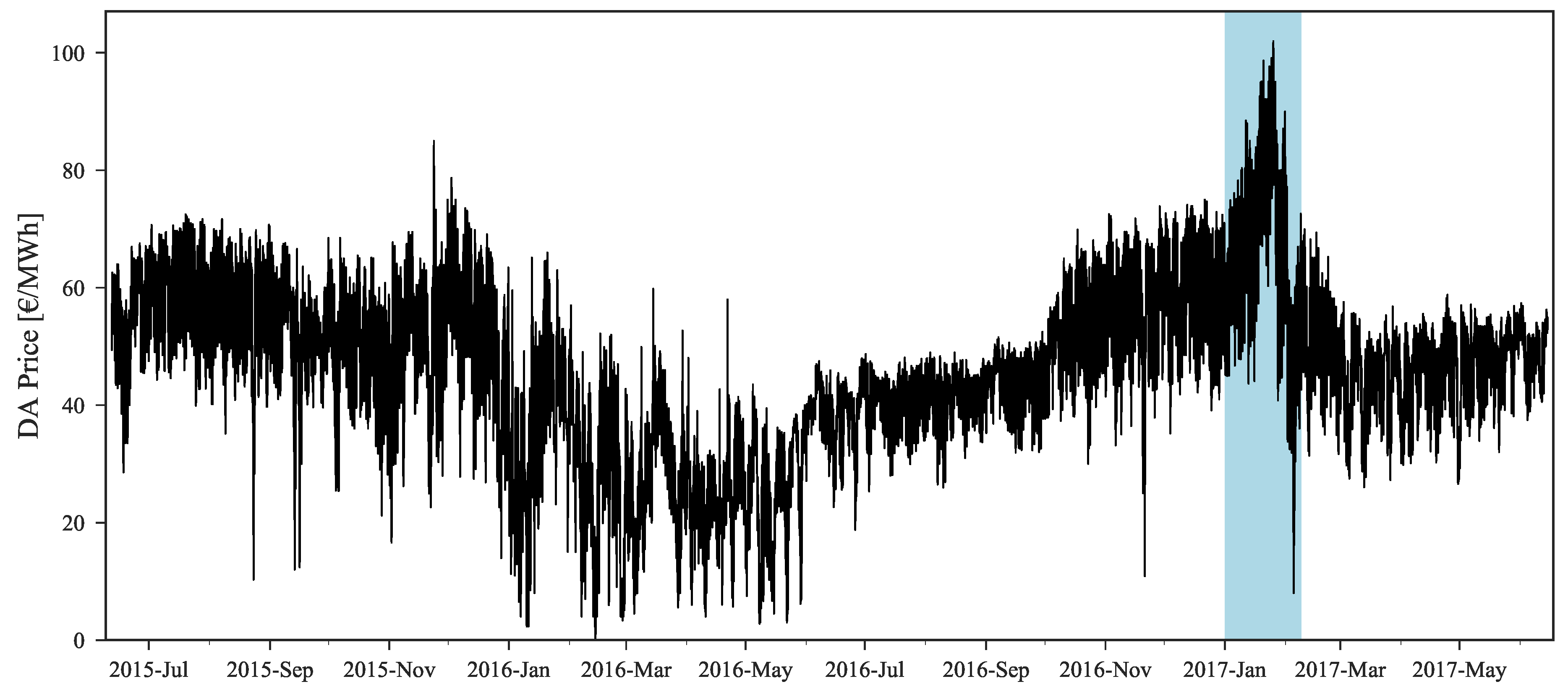
The original forecast completely misses during this period. This can be explained by analyzing
Figure 2 where it is possible to observe that this price range cannot be found in the historical dataset, which impacts the performance of statistical learning methods like GBT. With the information from daily average price forecasts it is possible to capture the trend of observed prices and then rescale the original forecasts for these periods, even without any past reference in the historical dataset.
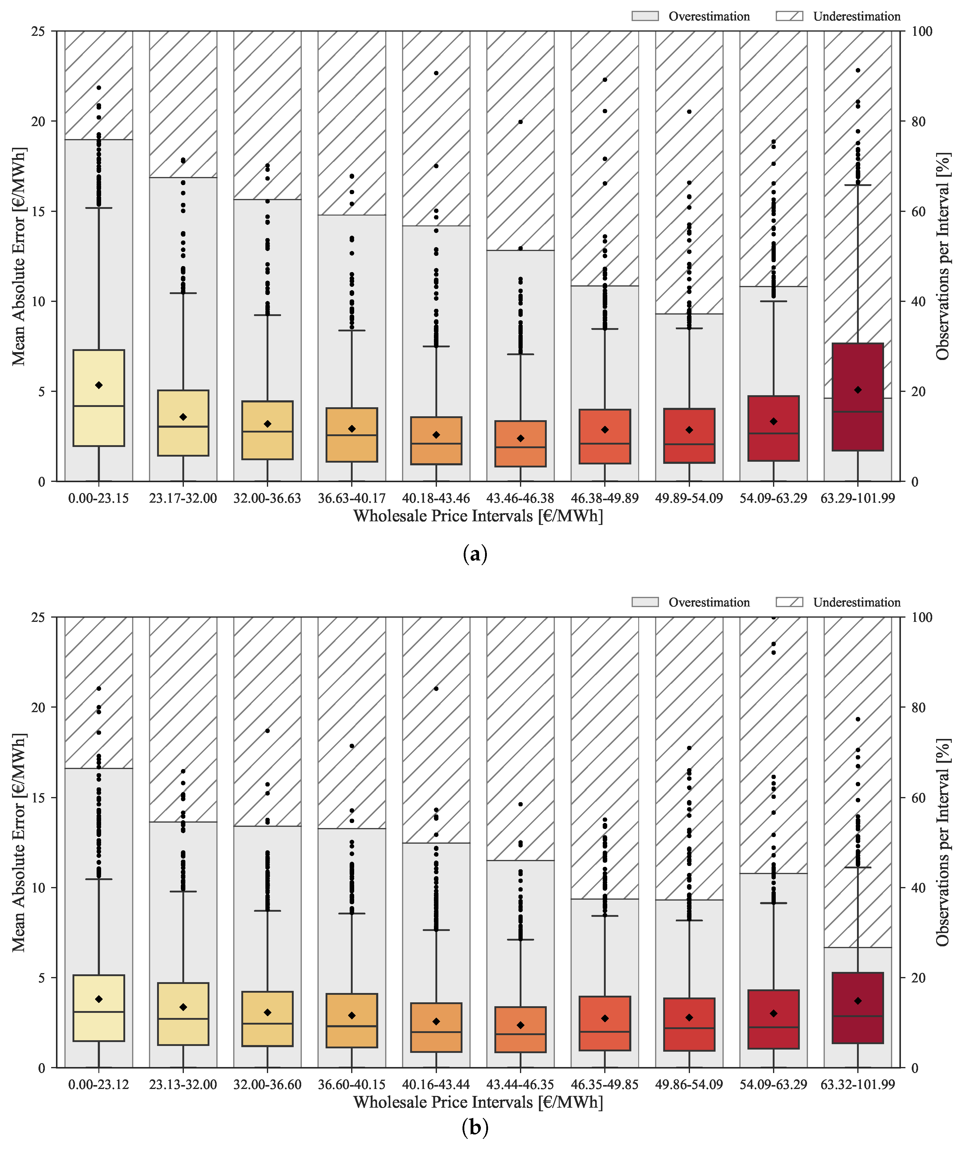
The improvements provided by the rescaling method throughout the complete range of prices are depicted in the boxplots of
Figure 12. These boxplots show the MAE distribution divided by ten equally distributed price classes, as well as the percentage of forecasts with under and overestimation. The top plot corresponds to the original forecasts, while the bottom plots concerns the rescaled forecasts.
The original forecasts have a tendency to overestimate in low price regimes and underestimate in high price regimes. This bias is mitigated by the rescaling process as demonstrated in the bottom boxplot. As previously mentioned, the improvement obtained by rescaling the forecasts is lower for medium price levels. However, it is substantially high for low/high price levels as showed by the MAE reduction between the two boxplots.
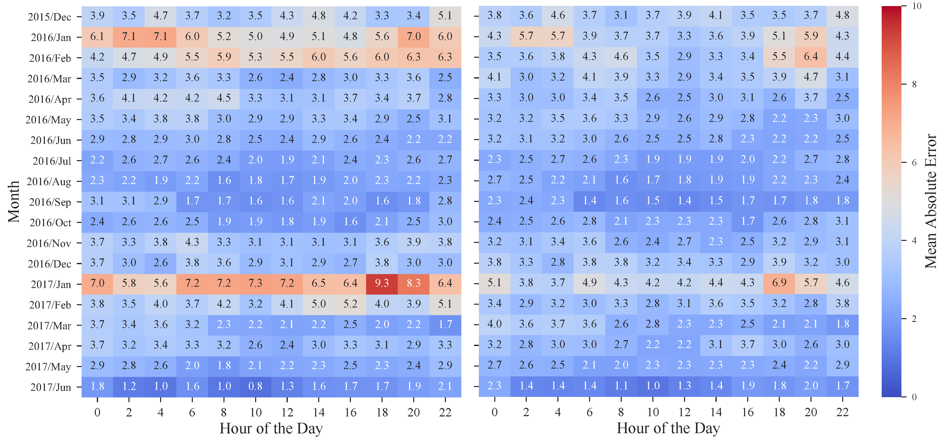
The benefits of the rescaling procedure are also emphasized by the heatmaps depicted in
Figure 13, in which the MAE values for each hour and month of the period under evaluation are presented. Once again, and by revisiting
Figure 2, it is possible to observe the significant improvement obtained in weeks with high prices. In January 2017, the MAE was ranging from 5.6 to 9.3 €/MWh while after applying the rescaling theses values decreased to 3.7–6.9 €/MWh. Furthermore, these results also show that, as the historical dataset increases, the forecasting error has a tendency to decrease, with the exception of atypical price periods.
4.4. Numerical Results: Intraday Markets
As mentioned in
Section 3.2, it was verified that the information about hourly prices of the daily session and previous intraday sessions is highly valuable and must be considered in the forecast model. In this subsection, four distinct type of models that synthesize different sets of variables are evaluated:
IM1—Selection of historical and forecasted system variables (see model M
final of
Table 5) combined with price information of the previous market session.
IM2—Forecasted system variables (see Future [
D + 1] information in
Table 2) combined with prices from previous market session.
IM3—Prices from previous market session.
IM4—Combination of the clearing prices of every preceding session (i.e., for ID2 the prices of ID1 and DA are used as explanatory variables).
Models IM1 and IM2 were defined to assess the importance of system variables (or exogenous information) to the forecasting skill. Models IM3 and IM4 are exclusively composed by previous daily and/or intraday session prices data. Model IM4 corresponds to
defined in Equation (
11) where, for each session
i, the previous daily and intraday market sessions prices are included. In contrast, IM3 only includes information from the previous session (
). These models were defined to verify the importance of this information when included alone, independently of any exogenous variables. All models accommodate calendar variables (see
Table 2) as it helped to capture some daily and weekly periodicity.
Table 7 summarizes the point and probabilistic forecasting skill scores for the intraday models IM1, IM2, IM3 and IM4.
An analysis of the table shows, for each session, that there is a high similarity between the evaluation scores, with MAE, RMSE, MAPE and CRPS presenting values with similar order of magnitude.
Comparing the results of models IM1 and IM2, it is hard to settle which information provides the most accurate price forecast. The discrepancy between models only starts being noticeable for sessions subsequent to ID3, where model IM2 starts to outperform the first in every score. However, a comparison between these two models and IM3/IM4 shows that previous market session prices are sufficient and offer better forecasts for the intraday market (i.e., close to 1% improvement of IM3 over IM2 and IM1 in ID1). This observations reveal that exogenous information is not critical to achieve a good forecast quality in this type of market.
An overview of the six intraday sessions results reveals a general decrease in the forecast accuracy from ID2 to ID6 (see the upward trend on MAE, RMSE, MAPE and CRPS errors), with exception of ID4 where the models presented better performance. An hypothesis for this increase in the error relates to the trading liquidity of these markets, that decreases as it approximates to the last session. In these low liquidity periods, higher price volatility is verified along with some cases where the prices reached its maximum value of 180.3 €/MWh.
Regarding ID1, it is important to remember that it includes the last three hours of the current day (day D). These hours are the last opportunity for adjustments in day D (e.g., the Portuguese transmission system operator names this period intraday 7) and corresponds to the time period with the lowest liquidity, which makes it specially hard to forecast. Higher errors on these hours increase the overall average forecast error of session ID1.
Compared to the day-ahead session forecasting skill (see
Table 6), it is possible to verify that the forecasts for intraday sessions exhibit substantially lower errors in point and probabilistic forecasts. This difference occurs mainly due to the available price references when the forecast is generated. For intraday sessions, hourly prices from the previous sessions (intraday and day-ahead) are powerful explanatory variables and are immediately available. On the other hand, for the day-ahead market, the only reference is the settlement price of daily futures contract that does not encompass information about hourly price variations. Moreover, the explanatory power of the previous day prices is considerably lower when compared to the price from previous intraday sessions.
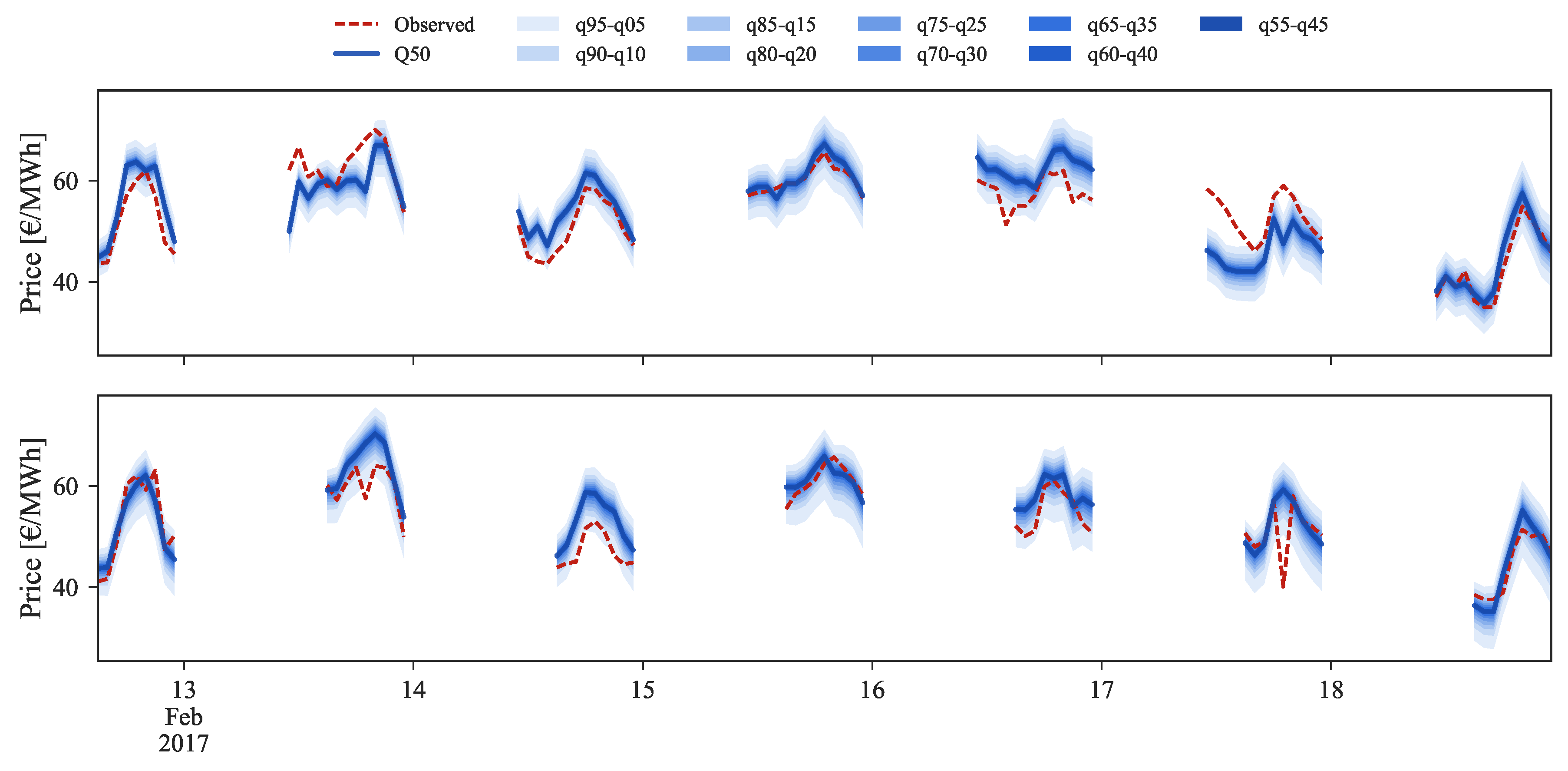
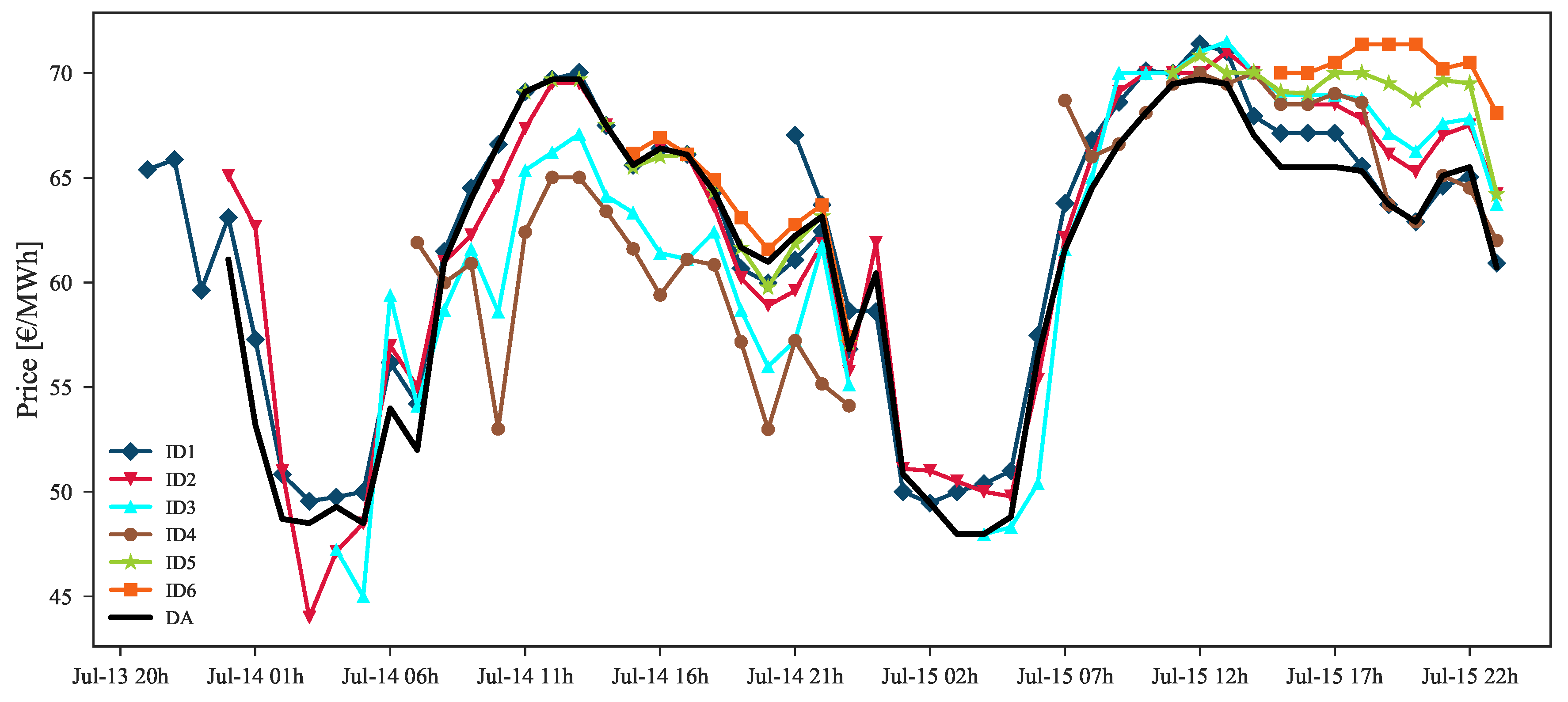
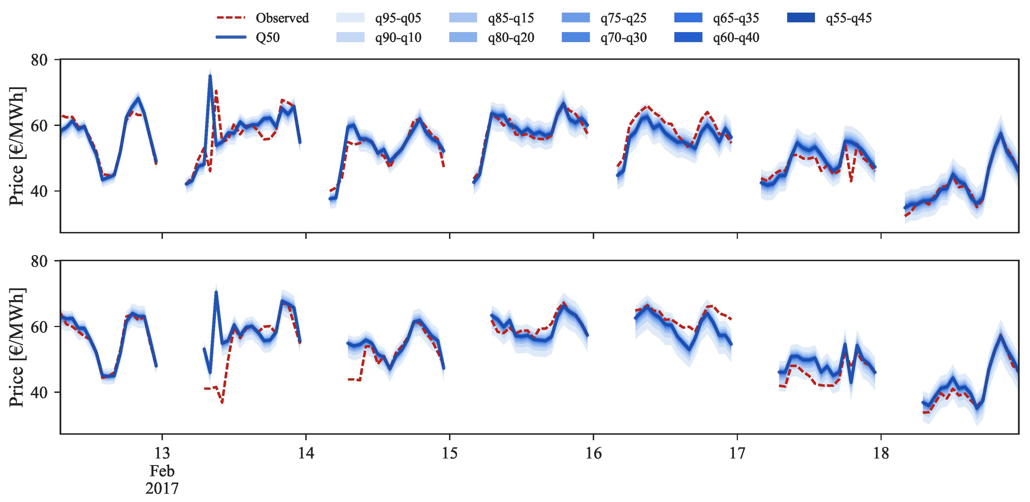
Figure 14,
Figure 15 and
Figure 16 show probabilistic hourly price forecast time series for intraday sessions of days 13 to 19 February 2017, generated with model IM3.
An analysis of the plots shows that sharp probabilistic forecasts are generated for every lead time. These high sharpness levels are verified in the forecasts generated by each of the four models, being slightly inferior for IM1 and IM2. For these models, some improvements are verified in the calibration for ID1, ID2 and ID3 sessions, resulting in lower CRPS values. These results indicate that it would be advisable to generate point forecasts with a model exclusively based in past sessions prices (IM3, IM4), complemented with probabilistic forecasts generated with a model that integrates exogenous information (IM1, IM2). However, the relation between quality and simplicity is prioritized in this work. With that rationale, models IM3 and IM4 were preferred as they are capable to produce quality forecasts with the minimum number of explanatory variables.
As mentioned before, price data from previous sessions is the core information for intraday price forecasts. Yet, it is important to note that this dependency on the past session prices might compromise the performance for periods characterized by large price changes between sessions. For instance, intraday sessions 1 to 4, on 14 February 2017, depict a situation where, for the first half of the day, distinct values in price are observed in all sessions. A comparison between ID1 and ID2 observed and forecasted prices (red dashes and blue line in
Figure 14) demonstrates that the model is unable to predict the price spike verified at 8:00 of ID2. This occurs due to the model dependency on ID1 where no price spike was verified. A similar price spike occurs at the following hour in ID3, which was forecasted with an offset due to the forecasts dependency on the observed price from ID2. In contrast, for the same hours ID4 presents a significant decrease in price when compared to the preceding sessions, which was then impossible to forecast by our model.
Although some of these sudden price shifts periods are impossible to model by the forecast uncertainty, the remaining lead times are forecasted with high point and probabilistic forecast accuracy.
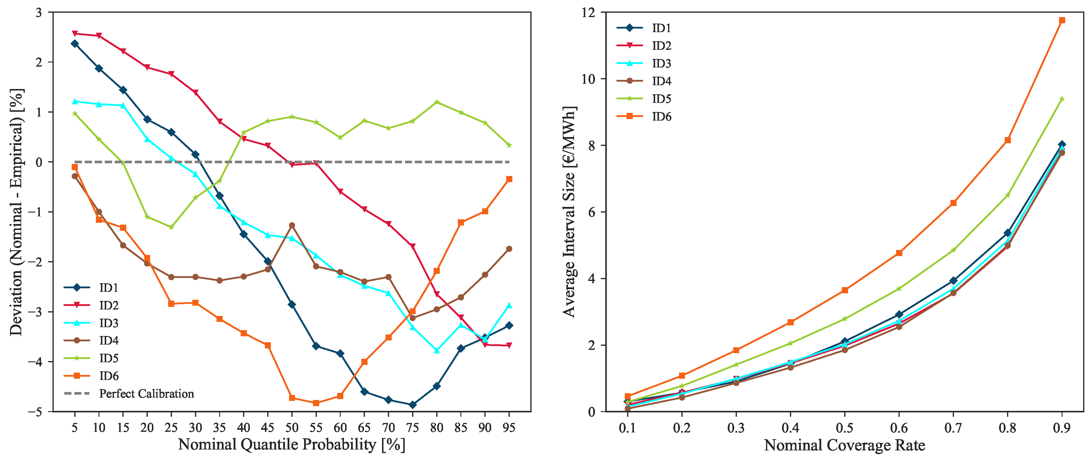
Figure 17 depicts the calibration and sharpness of the forecasts generated with model IM3 for all the intraday sessions.
The figure shows that, although sharp probabilistic forecasts are being produced for each intraday session (i.e., ID1, ID2, ID3 and ID4 close to 8 €/MWh average Q05–Q95 interval size), a good calibration is also maintained thorough every session, i.e., deviations from perfect calibration below 5% for all market sessions. These results confirm that the uncertainty of probabilistic forecasts is being correctly modeled, encompassing the observed hourly price values. As expected, in order to contain the increase in price volatility verified in sessions ID5 and ID6, lower sharpness levels can be noted for these sessions (see the higher average interval size for ID5 and ID6 depicted in
Figure 17 right side plot).
5. Conclusions
This paper describes a point and probabilistic statistically-based forecasting methodology for day-ahead and intraday electricity markets. The case study was the Iberian electricity market, characterized by high integration levels of different renewable energy technologies. The proposed forecasting methodology was not driven by the choice of the statistical learning algorithm. Instead, two robust statistical algorithms from the state of the art were used: gradient boosting trees and linear quantile regression. The core contributions to improve forecasting skill were: (a) careful selection of explanatory variables with special emphasis to the information from the futures contract trading; (b) post-processing of forecasts by exploiting the forecasted daily average price. For intraday markets, this work showed that high quality probabilistic forecasts can be obtained by just exploring the prices from previous sessions.
The results showed highly accurate point and probabilistic forecasts for both day-ahead and intraday markets. In terms of point forecast, the mean absolute error was 3.03 €/MWh for day-ahead market and a maximum value of 2.53 €/MWh was obtained for intraday session 6. The probabilistic forecast results show sharp forecast intervals and deviations from perfect calibration below 7% for all market sessions.
All the data used in this work is from public repositories, which allows reproducible research and shows that accurate price forecasts can be obtained without purchasing expensive data sources (e.g., wind power forecasts, weather predictions). Although tested for the Iberian electricity market, the methodology is generic and can be replicated to other European countries. However, the final set of explanatory variables and the forecasting skill might be different, in particular for electricity markets with low integration of hydropower and/or renewable energy.
Finally, the present paper was focused in forecasting the spot electricity prices and a topic for future work is to forecast operating reserve prices which, according to [
51,
52], show higher variability and more frequent extreme spikes. Other topics for future work are mid-term probabilistic price forecasting and the test of alternative models, like the autoregressive logit models described in [
53] or deep learning techniques with high potential to extract information from raw input variables.


