Development of a Multi-Objective Sizing Method for Borehole Heat Exchangers during the Early Design Phase


1
Department of Architectural Engineering, Inha University, Incheon 22212, Korea
2
GS E & C Building Science Research Team, Baekokdae-ro 388, Yongin 17130, Korea
*
Author to whom correspondence should be addressed.
Sustainability 2017, 9(10), 1876; https://doi.org/10.3390/su9101876
Submission received: 30 September 2017
/
Revised: 13 October 2017
/
Accepted: 14 October 2017
/
Published: 19 October 2017
(This article belongs to the Section Energy Sustainability)
Abstract
:Ground-source heat pump (GSHP) systems coupled with borehole heat exchangers (BHEs) are widely used as a renewable energy source. However, the high initial costs to install the BHEs still acts as an obstacle in the expansion of these renewable energy source systems. Specifically, in South Korea, a typical residential type corresponds to an apartment building with a high building-to-land ratio for land efficiency, and thus the space to install the BHEs is usually insufficient. Furthermore, the high initial cost issue of BHEs makes it difficult to ensure the feasibility of GSHP projects in this type of a situation. This study proposes a novel BHE sizing method to support the process of sizing energy sources in the design development phase of a construction project. Life cycle cost (LCC) analysis was combined with a tool to optimize BHE sizing by considering various economic aspects. Entering water temperatures (EWT) to heat pumps in conjunction with the LCC were used to define objective functions. Consequently, Pareto optimal solutions were obtained on the EWT–LCC plot. A group of Pareto optimal solutions forms a Pareto-curve, and each point on the curve indicates a possible sizing scenario or alternative. Finally, it is possible for decision makers to compare the solutions that include both technical and economic information. The Pareto optimal solutions are expected to support proper decision making in the early design phase.
1. Introduction
Borehole heat exchangers (BHE) are commonly used for ground-source heat pump (GSHP) systems. The BHEs are usually installed in the ground with a depth range from 50 to 200 m because the ground temperature in the depth is less fluctuated over the year [1]. The BHEs are also used in borehole thermal energy storage (BTES) systems [2] to store extra heat during summer and use the heat during winter [3]. One of the advantages of the BHEs is that they reduce the required installation area especially in high-density urban areas [4,5] as they are vertically installed in the ground.
In South Korea, the BHEs are not frequently used despite of the advantage mentioned before. One reason is the lack of enough space to install the BHEs around the buildings. A conventional residential type in South Korea includes high-rise apartment buildings, and the apartments are usually built in small and complex urban areas. According to the Korean population and housing census report (2015) [6], around 61.6% of residential buildings correspond to the high-rise apartment. Legally acceptable building-to-land ratio ranges from 50 to 70% for residential areas, and it can be increased up to 90% for residential–commercial apartments [7]. Many recent Korean building projects tend to adopt higher building-to-land ratio in order to maximize their land efficiency. Consequently, the BHE installation is limited in many Korean construction projects because there is not sufficient space to ensure their building loads.
The other reason is that there are not proper methods to optimize BHEs in the limited space from their performance and cost perspectives. The conventional sizing tools use a required total length of BHEs to determine their installation space. However, the tools yield a single solution with a fixed value of the BHE design parameter, entering water temperature (EWT). This results in hasty ruling out of BHE option in early design process because the single solution does not provide enough alternatives to make reasonable decision regarding the system. The alternatives can be obtained by using a large range of permissible EWT values and consequently give various sizing results and cost options. Therefore, a novel BHE design tool to consider multiple objective functions and generate multiple BHE sizing solutions is required to support proper decision making in the early design process.
The BHE sizing process is performed during the design development step which is one of the four steps of the construction design phase [8] as shown in the Figure 1. The design development step is considered as an early design phase in conjunction with the first two steps, pre-design and schematic design phases. Possible energy systems are reviewed and selected in the design development step. The impact of decision making is more significant in the early stage of the project, and thus design changes based on value engineering (VE) and life cycle cost (LCC) analysis frequently occur in the design development phase [9,10].
In order to support a proper decision making process in the early design phase, various design alternatives must be reviewed with respect to cost and technical evaluations. A multi-objective optimization can be a solution for this type of purpose. Few studies were conducted to optimize the sizing of BHEs. Sayyaadi et al. [11] used the total revenue requirement (TRR) method by using a multi-objective genetic algorithm, MOGA, by defining the thermodynamic and thermoeconomic objective functions. Huang et al. [12] also performed design optimization of BHEs for decision making purposes. They performed the mathematical modelling of BHEs and performed MOGA in Matlab to derive entropy generations. However, the BHEs models used in both studies are unable to completely account for thermal interference effects among BHEs and especially for irregular borefields.
To account for the thermal interference effects, the Kavanaugh method [13] proposed by the American Society of Heating, Refrigerating, and Air-Conditioning Engineers (ASHRAE) [14] uses a penalty temperature. Eskilson’s ground response function, g-function, was proposed for a more accurate calculation of the effects [15]. The models are extensively used for sizing BHEs, but they are hardly able to be integrated with optimization algorithms.
A well-known BHE model is the Duct Storage (DST) model [16] that considers the thermal interference effects even for a large number of BHEs. The model is implemented in Transient System Simulation (TRNSYS) tool [17] which is easily combined with optimization algorithms such as GenOpt or Multiopt2 [18,19]. However, the DST model was developed only with the purpose of cylindrical borehole configurations as it was proposed for simulating BTES systems [2]. Bertagnolio et al. [20] proposed a possibility of describing I-shape borefield configurations with the DST model by modifying a DST parameter.
The objective of this study involves developing and implementing a multi-objective optimization sizing method of BHEs using the TRNSYS to generate multiple alternatives in the early design phase. This study specifically targets irregular borehole configurations that are frequently encountered in Korean construction projects. A method to adjust the DST model parameter is also proposed to describe the irregular borefields as an incremental work of the previous model [20]. The development process is detailed in the following sections.
2. Proposed Methodology
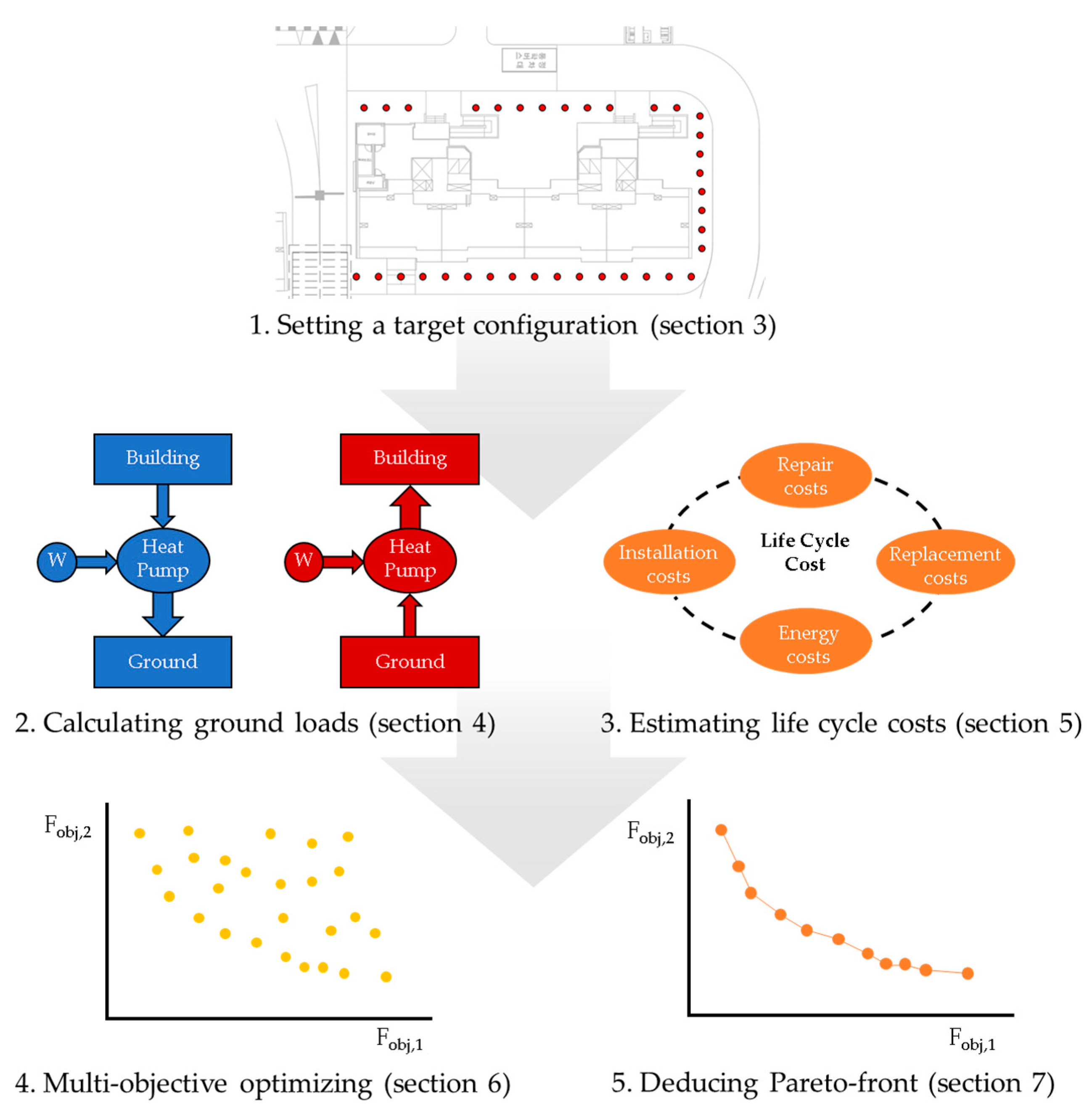
The proposed method of multi-objective optimization to design BHEs is presented as shown in Figure 2. First, possible borehole configurations apt for the target construction site are pre-described using the parameter modification method presented in the Section 3. Second, ground loads are calculated based on the building loads (Section 4). Third, cost information for a life cycle costs (LCCs) analysis is prepared to calculate 20-year net present values (NPV20) and energy cost with variable COPs (Section 5). Then, the setting method for the multi-objective optimization is presented in the Section 6. Finally, Section 7 shows how to run simulations and obtain a Pareto-front under given conditions.
3. TRNSYS Duct Storage (DST) Model
As mentioned in the previous section, the DST model was developed for BTES systems by using BHEs [16]. Specifically, it is considered that BHEs are regularly placed in a cylindrical borefield as shown in Figure 3. This assumption is acceptable for common BTES systems. The DST model was implemented in the TRNSYS TESS library as Type 557 [21]. The DST model calculates heat injection and rejection from or to the ground by accounting for heat transfer in the radial symmetry. Axial and radial grids are used for a numerical approach inside the storage volume (Figure 3) in which BHEs are regularly placed. Other similar grids are also generated for the entire ground domain that includes far field areas to calculate a global solution. However, an analytical solution is adopted for calculating local short-term heat transfer around a BHE. The fore-mentioned three solutions are combined at each time interval that is set inside the model. Further information on the model is detailed in an extant study [2]. The main input variables for the model correspond to the number of boreholes (N), borehole depth (H), and borehole spacing (B). The DST model automatically calculates the ground heat storage volume (VDST) as shown in Equation (1) as follows:
As previously mentioned, Bertagnolio et al. [20] reported the possibility of using DST for irregular borehole configurations. Simulation results for I-shape BHEs configuration were approximately fitted with existing ground heat exchanger models. They proposed modifying the cross sectional area of the VDST such that the circumference of the modified VDST is equal to the perimeter of the I-shape. Thus, the radius R in the cross section as shown in Figure 3 is modified to satisfy the following expression: . Therefore, the resultant cross sectional area of the VDST increases for the same number of BHEs in the I-shape borefield, and the thermal inference effects among BHEs are consequently mitigated as expected. The study by Bertagnolio et al. indicated that the modification method exhibited an error of 0.6 °C when compared to simulation results obtained by using Eskilson’s g-function for an 8 × 1 borehole configuration.
This study is inspired by the study by Bertagnolio et al., and we propose a similar modification method to describe a few specific borefields that are common in Korea such as L-, U-, and hollowed-rectangular-shapes. The idea is based on the fact that it is possible to divide the proposed borefields into a few I-shape borefields and that the thermal inference effects between I-shape borefields are less dominant when compared to adjacent BHEs in the same I-shape field. For example, the L-shape has two I-shaped borefields. This is expressed in Equation (2). Here, s represents the number of I-shape borefields. In the case of the I-shape, s becomes 1, and the equation corresponds to the same approach as that employed by Bertagnolio et al. [20]. The parameter s is set to two for an L-shape borefield, and U- and hollowed-rectangular-shapes are assumed as three and four, respectively. It is important to note that Equation (2) yields apparently different VModifying results for distinct s values when the other parameters are kept constant. This implies that the proposed method also accounts for the thermal inference effects among subgrouped I-shape borefields. A detailed verification is not considered in this study because this approach focuses on usefulness at the early design stage. For a selected option during the design development phase, it is necessary to perform detailed sizing with a conventional sizing tool in the construction documentation phase as shown in Figure 1. The expression is as follows:
4. Ground Load Calculation
The EWTs are one of the critical parameters in sizing and performance evaluation of the GSHP system, and they are determined by several conditions. First, the EWTs are affected by ground side conditions such as ground and grout properties, circulating fluid properties, and BHE configurations. These factors are determined by the design process of BHEs.
Conversely, the building loads and heat pump performances, such as COPs, also determine the variation in the EWTs. A combination factor of the building loads and COPs of heat pumps to the ground is termed as the ground load. This value is a key factor in designing the BHEs. It is necessary for the cooling ground loads to be rejected to the ground by means of BHEs and for the heating ground loads to be injected from the ground.
The ground loads are not sufficiently rejected to the ground when the total length of BHEs is excessively short for cooling. Consequently, the fluid temperatures in the U-tubes of the BHEs are increased, and the EWTs at the entrance of the source side of the heat pumps are likely to exceed the tolerated temperature of the heat pumps. This may result in a system failure. In contrast, long BHEs lead to a high performance of the heat pumps as the EWTs are significantly lower than the tolerated temperatures for the cooling period. However, this requires high initial costs.
The EWTs affect the COPs of heat pumps. Variable COPs are included in a function of the EWTs. The cooling and heating COPs are calculated in Equation (3). The coefficients α and β are obtained from the heat pump performance specifications provided by the manufacturer. Generally, lower EWTs increase the cooling COPs (COPc) while higher EWTs result in high COPs for heating cases (COPh). The expression is as follows:
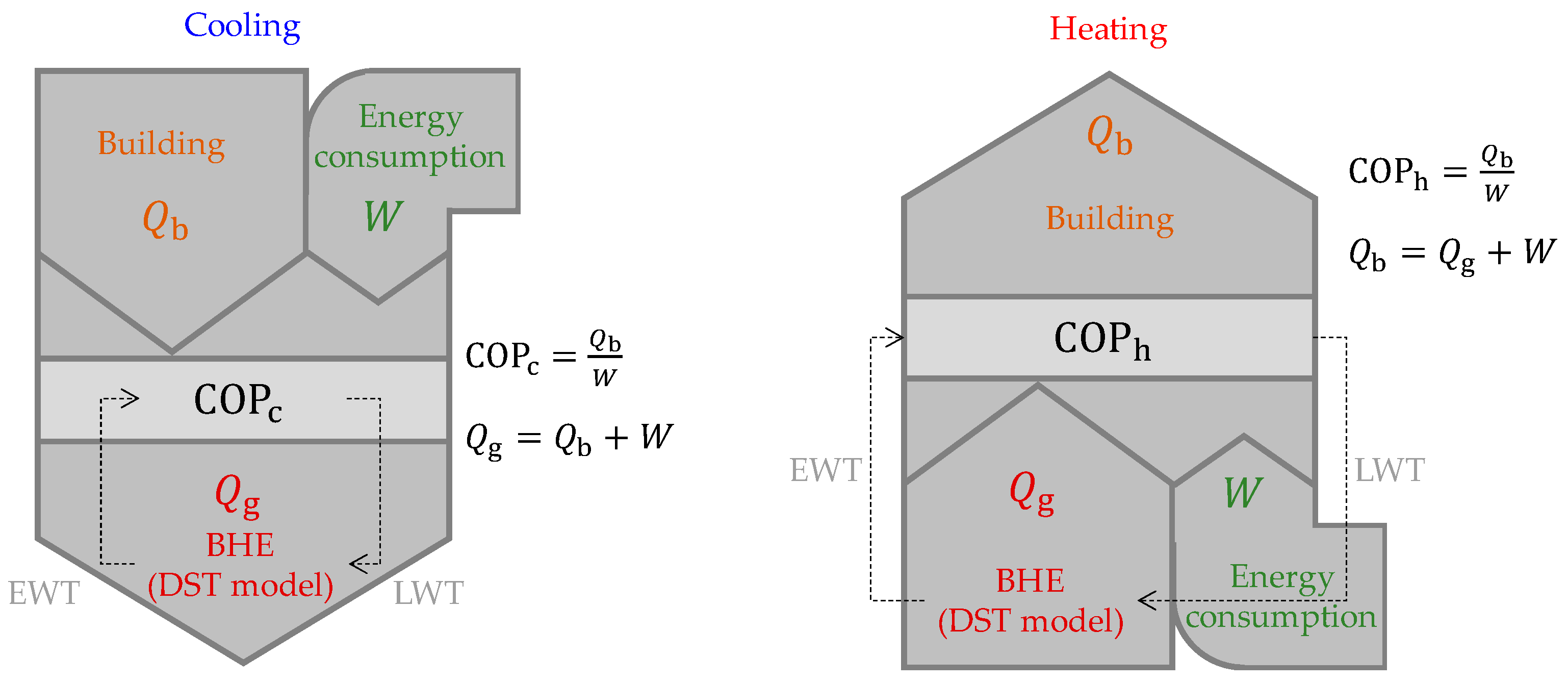
The COPs of heat pumps are also important in determining the ground loads. Based on the energy balance of the heat pump as shown in Figure 4, the ground load (Qg) belonging to the source side of the heat pump is calculated by a combination of the building loads (Qb) and the electric energy consumption (W) for the compressor. As shown in the figure, Qg exceeds Qb in the cooling cycle. However, Qg is lower than Qb in the heating cycle due to the direction of refrigerant circulation. This is expressed as shown in Equation (4).
The ground loads, Qg, are also used to calculate leaving water temperatures (LWT) from the heat pumps to BHEs as shown in Equation (5). The mass flow rate () and fluid specific heat (cp) also affect the calculation of the LWT. The symbol N represents the number of BHEs. In TRNSYS, the DST model calculates the EWTs for heat pumps from the LWTs in Equation (5). This details the mechanism through which the ground loads act in sizing simulations, and the calculated EWTs simultaneously determine the ground loads by using Equations (3) and (4). Therefore, several iterations are executed even at a given time step to obtain the converged EWTs and Qg in TRNSYS as follows:
When the ground loads are coupled with the EWTs, various maximum or minimum EWTs solutions are deployed by using multiple TRNSYS simulations launched by an optimization tool, and the corresponding sizing and energy costs are also evaluated by the economic analysis detailed in the following section.
5. Life Cycle Cost Analysis
Life cycle cost (LCC) analysis is an economic analysis for a component, system, or facility to determine the costs attributable to each alternative scenario over its economic life [22]. In the study, the target system corresponds to GSHP, and it is composed of several items as listed in Table 1 and based on an extant study [23]. The total construction cost for a GSHP is 3767.5 US dollars per Refrigeration Ton (RT), and the yearly repair and replacement periods are used to estimate maintenance costs. The same initial costs are applied for the replacements, and the repair cost is calculated by the ratio of the repair period to the replacement period.
Installation costs for items indicate the required cost for a single RT case. Specifically, in terms of the BHE capacity, it was assumed that 1 RT is equal to a depth of 50 m [24,25]. The correspondent cost ratio for each item is given in Table 1. The cost for installation is also termed as the initial cost. Therefore, it occurs once in the beginning, and repair and replacement payments occur periodically in the future. All future costs are adjusted at the present time to normalize both future and initial expenditures to obtain the net present value (NPV).
5.1. Net Present Value (NPV) Estimation
Generally, the thermal behavior of the BHEs changes continuously, and thus a long-term system evaluation is required to avoid system failure due to the excess EWTs with respect to the permissible range. Thus, several studies estimated the GSHP systems over 10 years or 20 years [2,7,26]. Hence, the present study uses 20 years as the simulation period, and the LCC evaluation period for possible scenarios is also set as 20 years. The NPV is applied for a 20-year period.
Equation (6) is used to calculate the NPV. Here, F denotes a future value corresponding to the expectation that a payment will occur in the future, and A denotes a uniform cost corresponding to the expectation that periodic payments will occur. A discount rate (i) of 3.26% is applied. This discount rate was reported in a recent domestic statistic report [27], and the value is used for facilities that are operated for a period exceeding 15 years. The expression is as follows:
5.2. Energy Cost
Energy costs are calculated by multiplying the energy consumption of heat pumps with the Korean unit price of electricity, namely $7.74 per 100 kWh. The energy consumption is derived from the energy balance as shown in Figure 4. Variable COPs used in Equation (3) are also applied in this energy cost calculation, and a similar equation is obtained for electricity consumptions by heat pumps as shown in Equation (7). Such a calculation method has also been used in other studies [28,29].
6. Multi-Objective Optimization
Optimization methods are classified into single-objective or multi-objective methods. The number of objective functions corresponds to the criterion for the classification. The single-objective optimization method is used to determine a single optimal solution in an economic or design optimization [26,30]. This optimization method is executed by defining an objective function that is set by design variables and the constraints of the variables. The single-objective optimization provides a single solution such that the value of objective function is minimized within the possible ranges.
Conversely, multi-objective optimization is useful in determining a set of optimal solutions that are termed as the Pareto-front [31]. The Pareto-front is used for optimizing design in conjunction with costs to provide information in a decision making process [32,33,34,35,36]. The Pareto-front is derived by using the logic that it is not possible to minimize an objective function without increasing another objective function. The present study employs the non-dominate sorting genetic algorithm-II (NSGA-II) as the multi-objective algorithm. From an initial generation to the frontier generation, the NSGA-II seeks the optimal solutions by using a stochastic optimizing strategy [31].
Table 2 shows the design variables for the multi-objective optimization of this study. The optimization uses continuous and discrete types of variables. The number of boreholes (N) and borehole depth (H) are designated as continuous variables to determine their optimal values and to subsequently calculate costs by using the same values. The borehole spacing is regarded as a discrete type of variable (e.g., 1 m and 2 m) for test cases to clearly see different optimization patterns on the Pareto-front curve. The borehole spacing can be a continuous variable if it is required. The range of borehole spacing is from 4 to 7 m for test cases. The range and the discrete borehole spacing values can be selected by designers based on the site conditions. The borehole spacing is an important indicator for decision makers because the final number of BHEs and the spacing can determine the required space of the construction site.
Specifically, a pair of objective functions related to the LCC and EWTs are used. The first objective function f1 involves minimizing the difference between the set EWT and simulated EWT and especially with respect to their maximum and minimum values for the cooling and heating seasons, respectively. The EWTc,set and EWTh,set are set to 30 °C and −5 °C, respectively. This objective function is shown in Equation (8).
The second objective function f2 uses the LCC results. As shown in Equation (9), the objective function is set such that it minimizes the LCC for a system operation over 20 years. The initial and maintenance costs and the energy costs are included in the equation. Similar studies [24,25] assumed that every 50 m in a BHE is equivalent to 1 RT, and thus a factor of 0.02 is multiplied in the objective function to simply calculate the LCC from the obtained total length of the BHEs.
As described, a few solutions are not minimized for an objective function but are close to the other objective function, thereby shaping the Parento-front. Thus, the selection of the set EWTs are not significant as the final results are broadly scattered around the values. The expression is as follows:
7. Results
7.1. Simulation Conditions
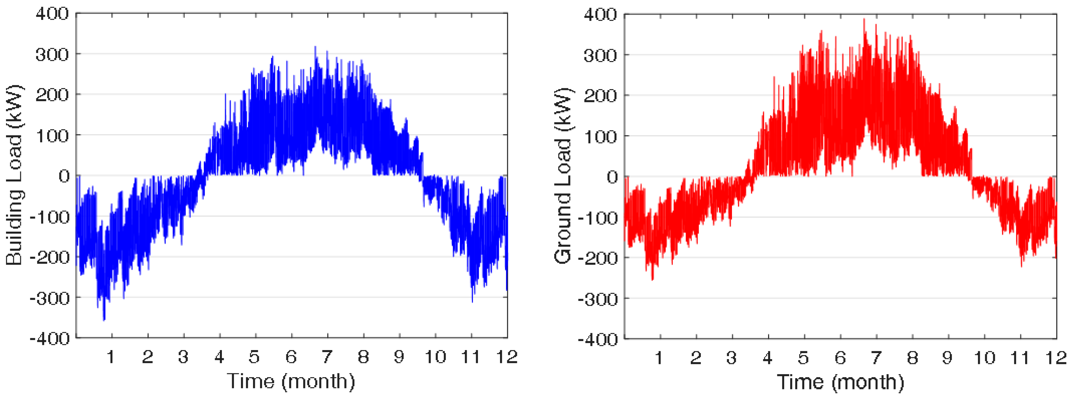
The test building corresponds to a 23-storey residential apartment in which 92 households reside. The building load was obtained under the heating and cooling set point temperatures corresponding to 20 °C and 26 °C, respectively, using Seoul TRY weather data [37]. Hourly building loads and ground loads are shown in Figure 5. Cooling loads are indicated with a plus (+) sign while heating loads are indicated with a minus (−) sign. The building loads appear balanced over the year although the ground loads exhibit cooling dominance due to the characteristics of the heat pump cycle as shown in Figure 3. The input parameters are listed in Table 3, and the values were used to calculate the appropriate solutions such as the number of BHEs and correspondent unit length of the BHEs. The total length of BHEs is calculated by multiplying the two design variables (N and H). Accordingly, EWTs are obtained for the given borefields configured by N, H, and B.
Table 4 shows the input parameters for the TRNSYS multi-objective tool, namely Multiopt2. A population size indicates the number of optimal solutions that are presented on the Pareto-curve. The number of generations indicates the number of descendants that are generated during an optimization run. In this work, the number is set to 10, seemingly smaller than common GA cases since the design variables are fewer (see Table 2). The transmission of genetics over generations follows a rule defined by the given crossing and mutation probabilities. Multiopt2 is run with the NSGA-II algorithm.
7.2. Simulation Results
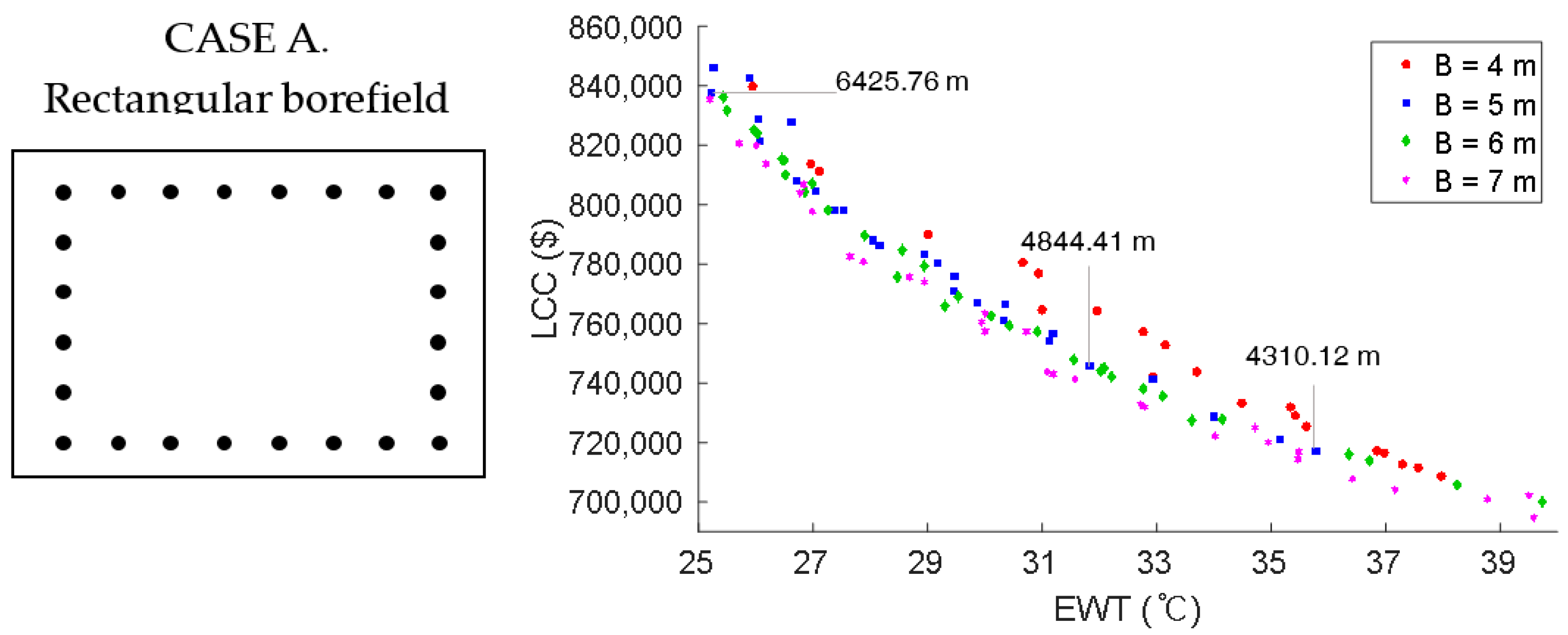
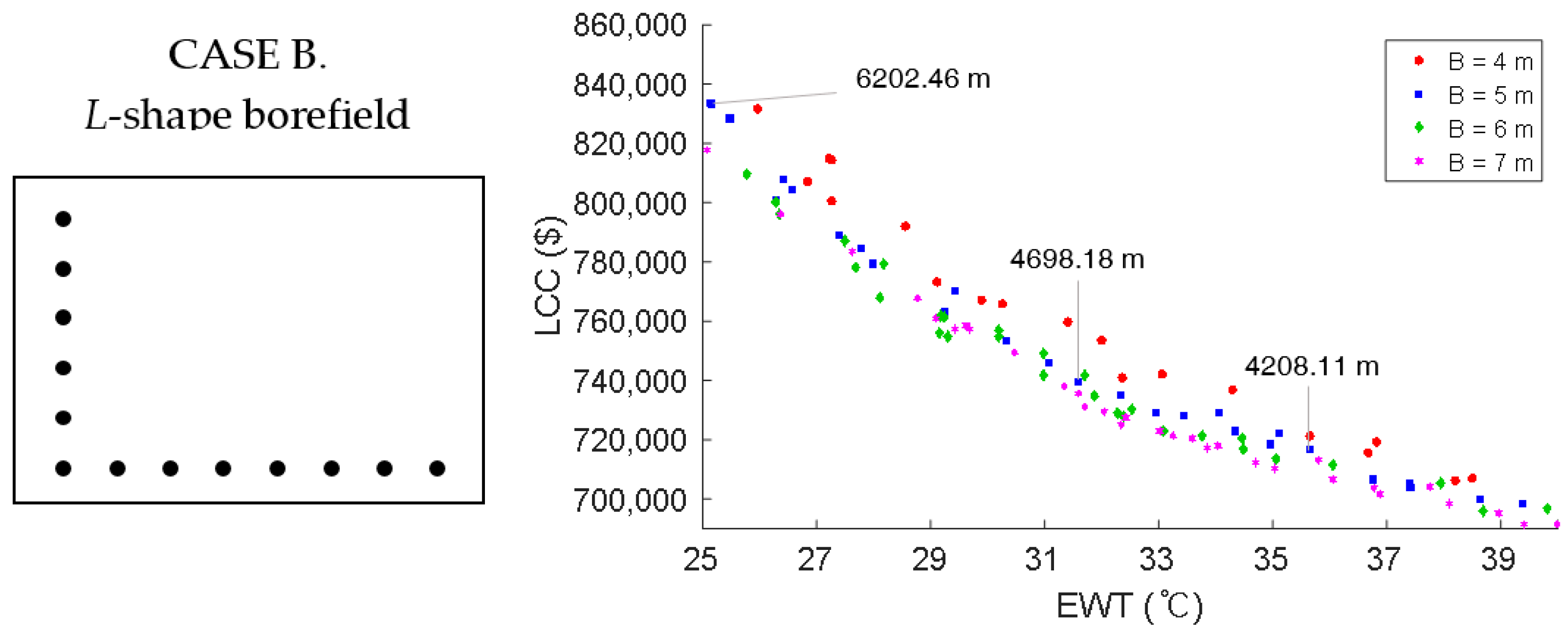
Hollowed-rectangular- and L-shape borefields were simulated as shown on the left side in Figure 6 and Figure 7, respectively. Pareto optimal solutions are obtained coupling a TRNSYS simulation project with Multiopt2. The right sides of the figures show the Pareto-curves ranging from 4 to 7 m of borehole spacing. The horizontal axis is set for EWTs defined as the first objective function, and the vertical axis is set for LCC that includes initial costs, maintenance costs, and energy costs. The ground loads are cooling dominant, and thus only a maximum EWT calculated with the DST model over the period was considered in Equation (8). A total of 40 Pareto optimal solutions were obtained with various maximum EWTs. Nevertheless, only cases between 25 to 40 °C are presented. Each point includes information on optimized design variables.
The results indicate that short BHEs spacing tends to result in higher LCC values for similar EWT values. With respect to the case with the maximum distance corresponding to 7 m, the LCC results are lower than those in the 4 m case. When the BHEs are closely placed, the thermal interference effects among BHEs become important, and thus the maximum EWT tends to increase in a cooling dominant case. Accordingly, the Multiopt2 may seek another design option, such as increasing the total length of BHEs, to decrease the maximum EWTs. This results in a higher LCC value. Therefore, the final Pareto-front points around the same EWT are placed as shown in Figure 6 and Figure 7. The curves in both Case A and Case B decrease when the EWTs increase. High design EWTs for cooling dominant cases lead to increased energy consumption for heat pumps, and thereby high energy costs. However, it is helpful to decrease the initial costs as the required total length of BHEs is considerably lower, and the initial cost for the system is high as shown in Table 1 when compared to the electricity cost.
In order to further investigate the results, three points are selected for each figure as shown in Figure 6 and Figure 7, and their details are listed Table 5. The points are placed at EWTs corresponding to 25, 32, and 36 °C, which represent all the cases corresponding to a spacing of 5 m. The total required lengths and LCCs in Case A (rectangular borefield) are always higher than those in Case B (L-shape borefield) as BHEs in Case A are more densely placed, and thereby result in increased thermal interference effects.
An option to increase design EWTs is reviewed when the construction site is characterized by insufficient space for installing BHEs. For example, shifting the maximum EWT from 25 to 36 °C reduces the required length by more than 30% (i.e., from 6425 to 4310 m) in Case A. The paired LCC results also aid in decision making.
With a single run of the multi-objective optimization tool, several LCC results were deployed with the corresponding system EWTs. The LCC results may be helpful for budget management while the EWTs and paired required lengths of BHEs with a specific borehole spacing are important for technical decision making for a given construction site.
The optimization results using NSGA-II were less fluctuated over generations. The last ninth and 10th generations’ results—the maximum, minimum, median, the 1st quartile, and the 3rd quartile values of total length of BHEs of the generations—are very similar each other (less than 1% difference in average). This is because a small number of design variables require a relatively small number of generations to optimize required values. Therefore, 10 generations are used for this study.
8. Conclusions
Existing BHE sizing methods are used to generate a single solution under fixed design parameter values. Based on the single solution, GSHP projects using BHEs are frequently refused even at an early design phase because a construction site is unable to provide sufficient space for an installation, and this frequently occurred in South Korea due to the highly permissible building-to-land ratios.
This study proposed a methodology that provides multiple design alternatives for sizing BHEs. Multi-objective optimization schemes were used to propose various sizing scenarios that consider life cycle cost analysis and to provide maximum or minimum EWTs for use in the early design stage and especially in the design development phase in which various possible energy systems are reviewed.
In this study, TRNSYS was selected to use the well-known DST model for simulating BHEs, and the Multiopt2 was combined with a TRNSYS simulation project to execute the multi-objective optimization. A modification method was also proposed to apply the DST model for a few typical irregular arrangements of BHEs that are frequently encountered in South Korea. The NSGA-II algorithm was applied for the optimization.
Objective functions were defined by using EWTs and LCCs. The EWTs considered variable COPs for detailed calculations, and LCCs were estimated by accounting for initial costs, maintenance costs, and energy costs. Design variables, borehole spacing (B), the number of boreholes (N), and borehole depth (H) were set under constraints to provide reliable sizing alternatives to decision makers.
Case studies were performed for a typical Korean apartment. The results revealed that multiple solutions formed a Pareto-front curve in a EWT–LCC plot. Some results are summarized as follows:
- -
- The optimization results included a large range of EWTs, but some reasonable EWTs could be useful for decision making.
- -
- When the BHEs were closely placed, important thermal interference effects among BHEs resulted in higher LCC values.
- -
- High design EWTs for cooling dominant cases lead to high energy costs, but the initial costs were more largely decreased.
- -
- The LCCs were lower even in the cases with short BHEs.
- -
- The NSGA-II algorithm showed fast optimization even with a few generations.
The proposed multi-optimization method can successfully give several design BHE design alternatives. From the test results, an option to increase the maximum EWT from 25 to 36 °C reduces the total required length of BHEs by 30%. This cannot be found with existing design tools where a single design EWT is generally adopted. Additionally, several other sizing options that are useful for a decision making are provided in a single plot. This might make it possible to adopt GSHP systems that would have been refused with the conventional design method.
The methodology proposed in this study to provide sizing solutions based on both economic and technical aspects is helpful in an early design stage. A sufficient review of possible scenarios and options in this phase may aid in avoiding high-cost design changes in the late design stage.
Acknowledgments
This study was supported by the INHA UNIVERSITY Research Grant (INHA-53357).
Author Contributions
Seung-Hoon Park, Yong-Sung Jang, and Eui-Jong Kim developed the model modification and multi-objective optimization methods. Jung-Yeol Kim applied the methods for the LCC calculation. Seung-Hoon Park drafted the manuscript, and it was revised by Eui-Jong Kim and Jung-Yeol Kim. The final manuscript was approved by all authors.
Conflicts of Interest
The authors declare no conflict of interest.
Nomenclature
| B | Borehole spacing (m) |
| N | Number of boreholes (-) |
| H | Borehole depth (m) |
| R | Borehole radius (m) |
| VDST | Heat storage volume in the DST model (m3) |
| VModifying | Modified heat storage volume in the DST model (m3) |
| s | Number of I-shape borefields (-) |
| α | Coefficient for cooling (-) |
| β | Coefficient for heating (-) |
| EWT | Entering water temperature (°C) |
| EWTc,set | Desired EWT for cooling (°C) |
| EWTh,set | Desired EWT for heating (°C) |
| EWTmax | Maximum EWT (°C) |
| EWTmin | Minimum EWT (°C) |
| COPc | Coefficient of performance for cooling (-) |
| COPh | Coefficient of performance for heating (-) |
| P | Cooling or Heating operation signal (-) |
| W | Work (kW) |
| Qb | Building load (kW) |
| Qg | Ground load (kW) |
| LWT | Leaving water temperature (°C) |
| Fluid mass flow rate (kg/s) | |
| cp | Fluid specific heat (J/kg·K) |
| NPV | Net present value (US $) |
| F | Future value (US $) |
| A | Annual payment (US $) |
| i | Discount rate (-) |
| n | Number of years (year) |
| f1 | First objective function (°C) |
| f2 | Second objective function (US $) |
References
- Rybach, L.; Sanner, B. Ground-source heat pump systems-the european experience. GHC Bull. 2000, 21, 16–26. [Google Scholar]
- Chapuis, S.; Bernier, M. Seasonal storage of solar energy in borehole heat exchangers. In Proceedings of the 11th International IBPSA Conference, Glasgow, UK, 27–30 July 2009. [Google Scholar]
- Cai, Y.; Xu, H.; Chen, S. Testing and analysis of the influence factors for the ground thermal parameters. Appl. Therm. Eng. 2016, 107, 662–671. [Google Scholar] [CrossRef]
- Soga, K.; Zhang, Y.; Choudhary, R. Potential of district-scale geothermal energy in urban cities. In Proceedings of the 1st International Conference on Energy Geotechnics, Kiel, Germany, 29–31 August 2016; CRC Press: Boca Raton, FL, USA, 2016. [Google Scholar]
- Bayer, P.; de Paly, M.; Beck, M. Strategic optimization of borehole heat exchanger field for seasonal geothermal heating and cooling. Appl. Energy 2014, 136, 445–453. [Google Scholar] [CrossRef]
- Population and Housing Census. Statistics Korea. Available online: http://kostat.go.kr/portal/eng/pressReleases/7/2/index.board (accessed on 17 September 2017).
- Korea Ministry of Government Legislation. Act on Planning and Utilization of the National Territory; Korea Ministry of Government Legislation: Sejong-si, Korea, 2012.
- University of California Office of the President. UC Facilities Manual. 2017. Available online: http://www.ucop.edu/construction-services/facilities-manual/volume-3/index.html (accessed on 21 September 2017).
- Fuller, S. Life-Cycle Cost Analysis (LCCA). National Institute of Building Sciences, an Authoritative Source of Innovative Solutions for the Built Environment. 2010. Available online: http://wbdg.org/resources/life-cycle-cost-analysis-lcca (accessed on 18 September 2017).
- Kerzner, H. Cost control. In Project Management: A Systems Approach to Planning, Scheduling, and Controlling, 9th ed.; John Wiley & Sons: Hoboken, NJ, USA, 2013; pp. 597–607. [Google Scholar]
- Sayyaadi, H.; Amlashi, E.H.; Amidpour, M. Multi-objective optimization of a vertical ground source heat pump using evolutionary algorithm. Energy Convers. Manag. 2009, 50, 2035–2046. [Google Scholar] [CrossRef]
- Huang, S.; Ma, Z.; Wang, F. A multi-objective design optimization strategy for vertical ground heat exchangers. Energy Build. 2015, 87, 233–242. [Google Scholar] [CrossRef]
- Kavanaugh, S. A design method for commercial ground-coupled heat pumps. ASHRAE Trans. 1995, 101, 1088–1094. [Google Scholar]
- ASHRAE. Geothermal energy. In ASHRAE Handbook—Applications; ASHRAE: Atlanta, GA, USA, 2015; Chapter 34. [Google Scholar]
- Bernier, M.; Chahla, A.; Pinel, P. Long-term ground-temperature changes in geo-exchange systems. ASHRAE Trans. 2008, 114, 342–350. [Google Scholar]
- Hellström, G. Duct Ground Heat Storage Model Manual for Computer Code; University of Lund: Lund, Sweden, 1989. [Google Scholar]
- Klein, S.A. TRNSYS, a Transient System Simulation Program; University of Wisconsin: Madison, WI, USA, 1979. [Google Scholar]
- Magnier, L.; Haghighat, F. Multiobjective optimization of building design using TRNSYS simulations, genetic algorithm, and Artificial Neural Network. Build. Environ. 2010, 45, 739–746. [Google Scholar] [CrossRef]
- Lu, S.; Tang, X.; Ji, L.; Tu, D. Research on energy-saving optimization for the performance parameters of rural-building shape and envelope by TRNSYS-GenOpt in hot summer and cold winter zone of China. Sustainability 2017, 9, 294. [Google Scholar] [CrossRef]
- Bertagnolio, S.; Bernier, M.; Kummert, M. Comparing vertical ground heat exchanger models. J. Build. Perform. Simul. 2012, 5, 369–383. [Google Scholar] [CrossRef]
- Pahud, D.; Fromentin, A.; Hadorn, J.C. The Duct Ground Heat Storage Model (DST) for TRNSYS Used for the Simulation of Heat Exchanger Piles; DGC-LASEN: Lausanne, Switzerland, 1996. [Google Scholar]
- Dell’Isola, A.; Kirk, S.J. Life Cycle Costing for Facilities; RSMeans: Rockland, MA, USA, 2003; Volume 51, pp. 20–64. [Google Scholar]
- Lee, I.G.; Kang, H.W.; Won, Y.M.; Kim, Y.S. Economic evaluation for heating and cooling system by using gas energy and geothermal energy based on LCC analysis. J. Archit. Inst. Korea Struct. Constr. 2011, 27, 161–168. [Google Scholar]
- Lim, H.J.; Song, Y.S.; Kong, H.J.; Park, S.K. Performance evaluation and economic estimation of ground source heat pump cooling and heating system. J. Energy Eng. 2004, 13, 296–300. [Google Scholar]
- Kim, S.G.; Kwon, S.W. The study of optimum method about the design and operating through a zero-energy house built in the existing building. New Renew. Energy 2015, 11, 49–59. [Google Scholar] [CrossRef]
- Zhang, C.; Hu, S.; Liu, Y.; Wang, Q. Optimal design of borehole heat exchangers based on hourly load simulation. Energy 2016, 116, 1180–1190. [Google Scholar] [CrossRef]
- Lee, J.; Kim, S.; Kim, G. An Expert Survey on the Social Discount Rate in Korea. Korean Energy Econ. Rev. 2016, 15, 207–237. Available online: http://www.dbpia.co.kr/Journal/ArticleDetail/NODE06651651 (accessed on 17 October 2017).
- Salvalai, G. Implementation and validation of simplified heat pump model in IDA-ICE energy simulation environment. Energy Build. 2012, 49, 132–141. [Google Scholar] [CrossRef]
- Miara, M.; Günther, D.; Leitner, Z.L.; Wapler, J. Simulation of an air-to-water heat pump system to evaluate the impact of demand-side-management measures on efficiency and load-shifting potential. Energy Technol. 2014, 2, 90–99. [Google Scholar] [CrossRef]
- Asadi, E.; da Silva, M.G.; Antunes, C.H.; Dias, L. A multi-objective optimization model for building retrofit strategies using TRNSYS simulations, GenOpt and MATLAB. Build. Environ. 2012, 56, 370–378. [Google Scholar] [CrossRef]
- Deb, K.; Pratap, A.; Agarwal, S.; Meyarivan, T.A.M.T. A fast and elitist multiobjective genetic algorithm: NSGA-II. IEEE Trans. Evolut. Comput. 2002, 6, 182–197. [Google Scholar] [CrossRef]
- Hayward, V.; Choksi, J.; Lanvin, G.; Ramstein, C. Design and multi-objective optimization of a linkage for a haptic interface. In Advances in Robot Kinematics and Computational Geometry; Springer: Dordrecht, The Netherlands, 1994; pp. 359–368. [Google Scholar]
- Miyazato, Y.; Tobaru, S.; Uchida, K.; Celestino, M.C.; Motin Howlader, A.; Senjyu, T. Multi-objective optimization for equipment capacity in off-grid smart house. Sustainability 2017, 9, 117. [Google Scholar] [CrossRef]
- Aláč, P.; Čulík, M. Multi-criteria decision-making model for the material flow of resonant wood production. Sustainability 2017, 9, 502. [Google Scholar]
- Toffolo, A.; Lazzaretto, A. Evolutionary algorithms for multi-objective energetic and economic optimization in thermal system design. Energy 2002, 27, 549–567. [Google Scholar] [CrossRef]
- Ko, Y.; Han, S. A duration prediction using a material-based progress management methodology for construction operation plans. Sustainability 2017, 9, 635. [Google Scholar] [CrossRef]
- The Korean Solar Energy Society. Available online: http://www.kses.re.kr/data_06/list_hi.php (accessed on 15 September 2017).
Figure 1.
Four steps in the construction design phase.
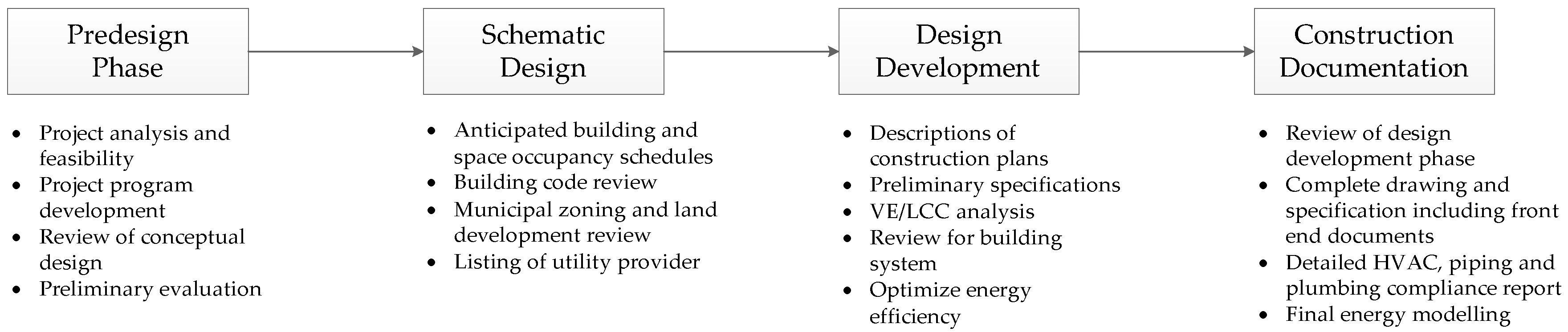
Figure 2.
Multi-optimization process presented in this study.

Figure 3.
Schematic of duct storage (DST) case with 19 boreholes.
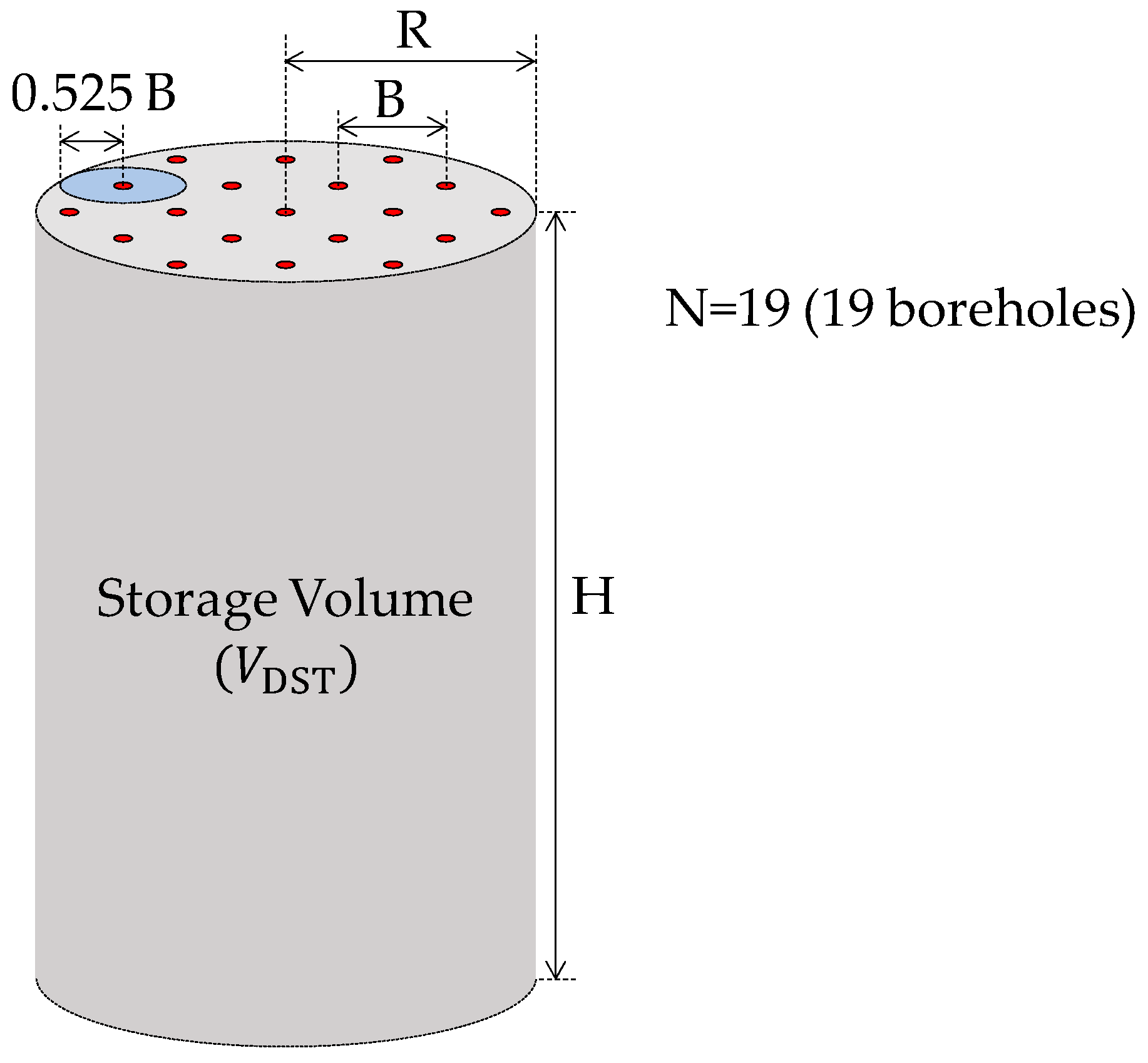
Figure 4.
Energy balance of the heat pump for cooling and heating cycles.

Figure 5.
Hourly building loads (left) and ground loads (right) over the year.

Figure 6.
EWT-LCC Pareto optimal solutions for a rectangular borefield (case A).

Figure 7.
EWT-LCC Pareto optimal solutions in the case of the L-shape borefield (case B).


Table 1.
Parameters for the life cycle cost analysis.
| Item | Cost Ratio (%) | Unit Cost for Installation ($/RT) | Repair Period (Year) | Replacement Period (Year) |
|---|---|---|---|---|
| Heat pump | 10.74 | 404.63 | 7 | 20 |
| Drilling & Trench | 45.42 | 1711.19 | - | - |
| Terminal unit | 6.41 | 241.50 | 6 | 15 |
| Pump | 2.15 | 81.00 | 3 | 20 |
| Pipe | 15.37 | 579.06 | 10 | 20 |
| Controller | 0.89 | 33.53 | 5 | 20 |
| Duct | 19.02 | 716.58 | 8 | 15 |
Table 2.
Design variables and constraints for multi-object optimization.
| Design Variable | Unit | Constraints | |
|---|---|---|---|
| Min | Max | ||
| Number of boreholes (N) | EA | 35 | 45 |
| Unit borehole depth (H) | m | 85 | 200 |
| Borehole spacing (B) | m | 4, 5, 6, 7 (discrete) | |
Table 3.
Input parameters for simulation.
| Parameters | Value | Unit |
|---|---|---|
| Building | ||
| Floor area | 72 | m2 |
| Number of households | 92 | - |
| Ground | ||
| Initial temperature | 10 | °C |
| Thermal conductivity | 2 | W/m·K |
| Thermal capacity | 2160.5 | kJ/m3·K |
| Thermal diffusivity | 0.08 | m2/day |
| Borehole | ||
| Borehole radius | 55 | mm |
| Borehole spacing | 4, 5, 6, 7 | m |
| Pipe center to center distance | 23.5 | mm |
| Depth | To be optimized | m |
| Desired EWT for cooling | 30 | °C |
| Desired EWT for heating | −5 | °C |
| Grout thermal conductivity | 2 | W/m·K |
| Header depth | 1 | m |
| Mass flow rate per boreholes | 0.2 | kg/s |
| Number of boreholes | To be optimized | - |
| Pipe radius (inner/outer) | 13/16 | mm |
| Pipe thermal conductivity | 0.4 | W/m·K |
| Fluid | ||
| Density | 1022 | kg/m3 |
| Specific heat | 3960 | J/kg·K |
Table 4.
Parameters for NSGA-II.
| Parameter | Value |
|---|---|
| Population size | 40 |
| Number of generations | 10 |
| Crossing probability | 0.7 |
| Mutation probability | 0.1 |
Table 5.
Calculated total lengths for different maximum EWTs and LCC values.
| Borefield | EWTmax ≈ 25 °C | EWTmax ≈ 32 °C | EWTmax ≈ 36 °C | |||
|---|---|---|---|---|---|---|
| Length (m) | LCC (US $) | Length (m) | LCC (US $) | Length (m) | LCC (US $) | |
| CASE A | 6425.76 | 846,075 | 4844.41 | 745,608 | 4310.11 | 717,099 |
| CASE B | 6202.46 | 833,252 | 4698.18 | 739,740 | 4208.11 | 716,661 |
© 2017 by the authors. Licensee MDPI, Basel, Switzerland. This article is an open access article distributed under the terms and conditions of the Creative Commons Attribution (CC BY) license (http://creativecommons.org/licenses/by/4.0/).
Share and Cite
MDPI and ACS Style
Park, S.-H.; Kim, J.-Y.; Jang, Y.-S.; Kim, E.-J. Development of a Multi-Objective Sizing Method for Borehole Heat Exchangers during the Early Design Phase. Sustainability 2017, 9, 1876. https://doi.org/10.3390/su9101876
AMA Style
Park S-H, Kim J-Y, Jang Y-S, Kim E-J. Development of a Multi-Objective Sizing Method for Borehole Heat Exchangers during the Early Design Phase. Sustainability. 2017; 9(10):1876. https://doi.org/10.3390/su9101876
Chicago/Turabian StylePark, Seung-Hoon, Jung-Yeol Kim, Yong-Sung Jang, and Eui-Jong Kim. 2017. "Development of a Multi-Objective Sizing Method for Borehole Heat Exchangers during the Early Design Phase" Sustainability 9, no. 10: 1876. https://doi.org/10.3390/su9101876
Note that from the first issue of 2016, this journal uses article numbers instead of page numbers. See further details here.