Article

Integrating Cellular Automata with the Deep Belief Network for Simulating Urban Growth

1
School of Earth Sciences, Zhejiang University, 38 Zheda Road, Hangzhou 310027, China
2
Zhejiang Provincial Key Laboratory of Geographic Information Science, 148 Tianmushan Road, Hangzhou 310028, China
3
Department of Geography, Kent State University, Kent, OH 44240, USA
*
Author to whom correspondence should be addressed.
Sustainability 2017, 9(10), 1786; https://doi.org/10.3390/su9101786
Submission received: 20 August 2017 / Revised: 29 September 2017 / Accepted: 29 September 2017 / Published: 2 October 2017
(This article belongs to the Section Sustainable Urban and Rural Development)

Abstract

:
Sustainable urban development is a focus of regional policy makers; therefore, how to measure and understand urban growth is an important research topic. This paper quantified the amount of urban growth on land use maps that were derived from multi-temporal Landsat images of Jiaxing City as a rapidly-growing city in Zhejiang Province from 2000–2015. Furthermore, a new approach coupled the heuristic bat algorithm (BA) and deep belief network (DBN) with the cellular automata (CA) model (DBN-CA), which was developed to simulate the urban expansion in 2015 and forecast the distribution of urban areas of Jiaxing City in 2024. The BA was proposed to obtain the best structure of the DBN, while the optimized DBN model considered the nonlinear spatial-temporal relationship of driving forces in urban expansion. Comparisons between the DBN-CA and the conventional artificial neural network-based CA (ANN-CA) model were also performed. This study demonstrates that the proposed model is more stable and accurate than the ANN-CA model, since the minimum and maximum values of the kappa coefficient of the DBN-CA were 77.109% and 78.366%, while the ANN-CA’s values were 63.460% and 76.151% over the 200 experiments, respectively. Therefore, the DBN-CA model is a potentially effective new approach to survey land use change and urban expansion and allows sustainability research to study the health of urban growth trends.

1. Introduction

A scientific understanding of land use change and urban expansion is required for policy makers to strategize and facilitate sustainable urbanization development. Land use change is influenced by the interaction of many driving forces, including demographic change, socio-economic development, natural factors, human behavior and government policies [1,2]. In this context, urban growth simulations have made an indispensably significant contribution towards facilitating sustainable development by urban planners, decision makers, economists and ecologists. Over the past several decades, a great deal of literature has focused on realizing the interactions between land use change and its driving forces using land use models. These include statistical approaches [3,4], system dynamics models [5], conceptual models [6], Markov chain [7,8], agent-based models [9], cellular automata (CA) approaches and the integration of these methods [10,11].
CA models simulate and predict a spatial-temporal and nonlinear dynamic system by defining simple local transition rules. The CA models have been shown to be powerful and popular land use change simulation tools [12,13]. The CA model was first applied to simulate and explore urban growth in Detroit (Tobler 1970) [14]. Since then, CA models have been widely utilized in research on land use change and urban expansion simulation [15,16,17,18,19,20,21,22,23]. However, it remains a significant challenge to specify the transition rules of CA. The objective of CA calibration is to obtain the best transition rules that allow for the most accurate simulated results [23,24]. Consequently, it is crucial to properly calibrate CA parameters to acquire more precise land use change results.
So far, a large number of methods has been developed to calibrate CA parameters. Some authors used the SLEUTH urban growth model developed by Clarke based on the cellular automata to simulate urban expansion [16,17,25,26]. However, the input layers of the SLEUTH model are slope, land use/land cover, excluded zones, urban areas, transportation network and hillshading, which do not consider population change and socio-economic development. Furthermore, while the five variable parameters of the SLEUTH independently range from 0–100, there are too many combinations that can influence model performance. Wu (1998) [27], Wu and Webster (1998) [28] defined a multi-criteria evaluation (MCE) method based on the analytic hierarchy process (AHP) to obtain transition rules. Specifically, whether a cell developed or not was determined by the comprehensive evaluation of various spatial variables. Nonetheless, CA calibration with MCE is highly affected by the subjective parameter setting. Therefore, a number of studies proposed a CA model based on logistic regression to deal with multi-factor problems [29,30]. However, logistic regression is more likely to overfit and has difficulty effectively determining the complex relationships among variables. Consequently, artificial intelligence, machine learning techniques (e.g., support vector machine) and global intelligent optimization algorithms were introduced into CA parameter calibration [22,31,32,33].
Li and Yeh (2002) [18] first integrated artificial neural networks (ANNs) with CA models to simulate land use change. They demonstrated that the ANN-based CA (ANN-CA) model can be successfully applied to land use change and urban expansion simulations, due to ANNs’ strong self-adaptiveness, self-organization and ability to learn and mimic complex nonlinear problems [2,19,21,32,34]. However, the conventional ANNs are weak in global searching and fall more easily into local optima. Hence, improving conventional ANNs or developing a new method to be coupled with the CA might offer better simulation precision.
In the past decade, deep learning has shown great success with speech recognition and image classification [35,36,
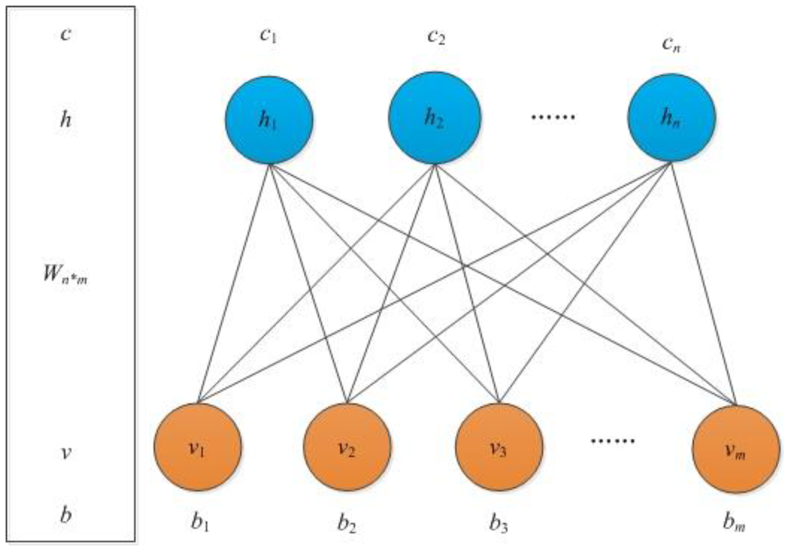
37]. As one of the dominant methods of deep learning, the deep belief network (DBN) has excellent feature detection abilities. When compared to the conventional ANNs, the DBN is more capable of interpreting complex mathematical models, due to a number of hidden layers for the feature detection [38,39,40]. Furthermore, it is much easier to express the non-linear, complex structures of the data in deep hidden layers. There is a fast, greedy, unsupervised learning algorithm that can initialize the weights of conventional ANN. DBN and ANN both employ a machine learning approach, which is not dependent on fixed functional relationships and is able to handle complex non-linear functions without any a priori knowledge of variable relationships [21,41]. Thus, the DBN overcomes ANN’s local convergence problem effectively. However, so far, only a few studies have combined DBN with the CA model to simulate land use change or urban growth.
Typical studies in urban growth used remote sensing and GIS techniques [2,27,41,42] and utilized three phases during model implementation: calibration, validation and prediction. Alsharif and Pradhan used a logistic regression model in the calibration phase from 1984–2002, validation from 2002–2010 and prediction for 2020 and 2025 for Tripoli, Libya [43]. Grekousis, Manetos and Photis integrated the ANN and fuzzy logic with GIS to calibrate, validate and predict urban growth for the Athens metropolitan area [41]. The ANN model in conjunction with other methods was also used to simulate urban growth including both calibration and validation [44,45,46]. Berberoğlu, Akın and Clarke compared urban modeling approaches, including logistic regression, regression tree, ANN and SLEUTH, to forecast the urban growth, and two calibration and prediction phases of these models were performed [47]. Riccioli utilized CA and Markov chains to examine the land use changes from 1990–2000, and it was validated for 2006 [48].
In this context, our research aims to propose a DBN-based CA (DBN-CA) model to simulate the spatial-temporal changes in non-urban land use, while the metaheuristic bat algorithm (BA) developed by Yang (2010) [
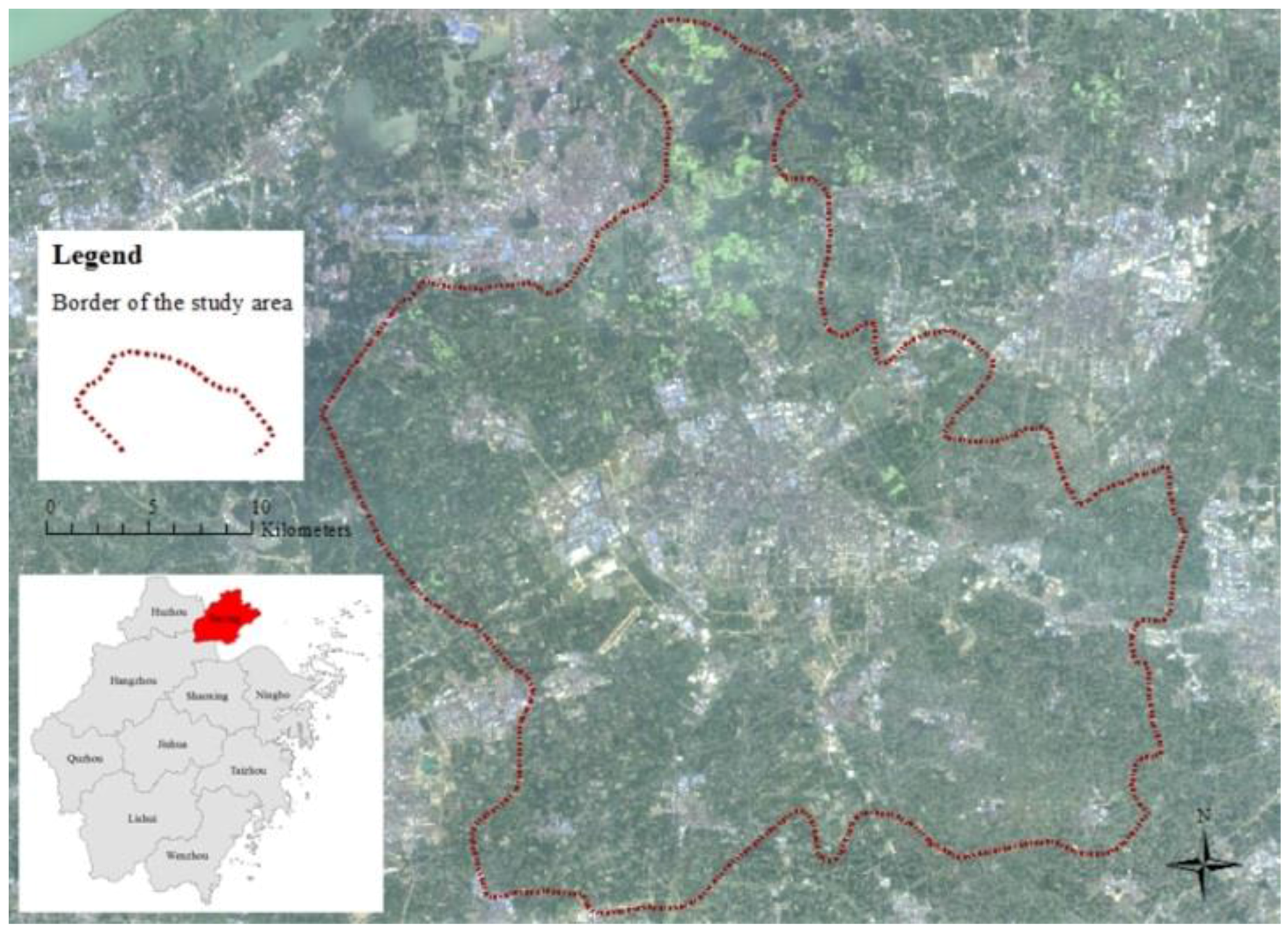
49] is proposed to obtain the best structure of the DBN, and the DBN training is used to achieve the best transition rules of non-urban change. The DBN-CA model involving data processing, DBN calibration, model validation and prediction is tested using a case study of urban growth for Jiaxing City, Zhejiang Province, China, in 2000, 2008, 2015 and 2024. We compare it to the ANN-based CA (ANN-CA) and demonstrate the effective simulation ability of the DBN-CA for the study area.
This paper is organized into five sections. The next section gives an introduction to the CA framework, the BA and DBN models and the framework of DBN-CA. Section 3 describes the study area and data. Section 4 describes the model implementation and discusses the results. Finally, Section 5 gives the major conclusions.

2. Methods

2.1. CA for Urban Growth Model

The history of the CA dates back to Von Neumann and Stanislaw Ulam’s study on the theory of self-reproducing automata in the 1940s [50]. A conventional CA consists of a dynamic discrete cell space, cell state, neighborhoods and transition rules. The future state of a cell is defined by a series of transition rules, which consider the cell’s initial state, neighborhoods and other driving forces. It can be formulated as follows:
S t a t e i j t + 1 = f ( N e i g h b o u r i j t , G l o b a l i j t , C o n s t r a i n t i j t ) = { u r b a n ,     p i j t > p t h r e s h o l d n o n u r b a n ,   p i j t p t h r e s h o l d
where S t a t e i j t + 1 is the state (urban/non-urban) of cell ij at time t + 1. p t h r e s h o l d is the threshold value generally predefined in the range of [0,1] [18]. By adjusting the threshold at each iteration, we can gradually approximate the total amount of non-urban land conversion demand during the simulation period. If p i j t > p t h r e s h o l d , the non-urban at time t changes to urban at time t + 1. Otherwise, the non-urban remains unchanged. The p i j t is related to all kinds of variables as shown in Equation (1). G l o b a l i j t represents global driving factors, such as socio-economic development and natural environmental conditions, including distance variables, elevation, population and GDP. C o n s t r a i n t i j t is the constraint conditions for land use change, such as the ecological zone and farmland zone. Here, we set the water as constraint data. N e i g h b o u r i j t is the neighboring cells of cell ij defined as an extended Moore neighborhood as follows:
N e i g h b o u r i j t = N u m ( { N i j t = ( N i t , N j t ) | | N i t N i t | + | N j t N j t | r , ( N i t , N j t ) Z 2 } )
where N i t , N j t are the coordinates of the neighboring cells at time t. N j t , N j t indicates the coordinates of the current cell. N u m is the number of neighboring cells, and r represents the radius of the neighborhood.
f is the transition function that finds the best combination of transition rules, while the models of DBN and ANN are developed in this study.

2.2. Deep Belief Network

Hinton (2006) [35] first proposed the deep belief network (DBN). DBN is a generative model that contains multiple hidden layers. A classical DBN model is composed of several restricted Boltzmann machines (RBMs), which are used for pre-training, and a conventional back propagation (BP) network for fine-tuning. An example of a DBN architecture is shown in Figure 1.
An RBM is an undirected probabilistic graphical model that consists of a layer of visible units ( v ) and a single layer of hidden units ( h ). There are no internal connections among units of the visible layer or among those of the hidden layer, while the visible units and hidden units are fully connected (Hinton, 2010). An RBM’s architecture is given in Figure 2. When given the visible units v = ( v 1 , v 2 , , v m ) and the hidden units h = ( h 1 , h , , h n ) , the energy function E ( v , h ) is defined as:
E ( v , h ) = i = 1 m j = 1 n v i w i j h j i = 1 m b i v i j = 1 n c j h j
where w i j is the connection weight between visible unit i and the hidden unit j, b i is the bias of visible unit i and c j is the bias of hidden unit j. Then, we get the joint probability distribution based on the specified energy function as follows:
p ( v , h ) = e E ( v , h ) Z
where Z = v , h e E ( v , h ) is the partition function. Since there are no connections within the same layer, the activation probability of hidden unit j is shown in Equation (3) when given the visible units v :
P ( h j = 1 | v ) = s i g m o i d ( c j + i v i w i j )
Since an RBM is symmetrical, given the hidden units h , the activation probability of visible unit i is:
P ( v i = 1 | h ) = s i g m o i d ( b i + j h j w i j )
where s i g m o i d ( x ) = 1 1 + exp ( x ) is the activation function.
The objective of the RBM is to find the best parameters θ = { w , v , h , b , c } using the stochastic gradient ascent. Hinton (2002) [51] developed a fast learning algorithm for the RBM called contrastive divergence (CD). An RBM can be trained as follows. First, initialize the visible units’ states as the training data and the parameters including the number of hidden units, learning rate α and the training period. Second, calculate the binary state of each hidden unit using Equation (5). Third, given the binary state of each hidden unit, calculate the probability of each visible unit using Equation (6). Then, a “reconstruction” is produced, reconErr = reconErr + || v v t ||, which represents the difference between the input data and the modeling data. Finally, output the connection weight w and bias b , c . The change in { w , b , c } is given by:
Δ w i j = α ( v i h j d a t a v i h j m o d e l ) Δ b i = α ( v i d a t a v i m o d e l ) Δ c j = α ( h j d a t a h j m o d e l )
where v i h j d a t a is the expectation of the observed data and v i h j m o d e l is the expectation of the modeled data.
According to the principle of minimum energy for the DBN architecture, the input of the next RBM is the output probability and states of the previous RBM. The fine-tuning procedure is that the conventional BP network received the output of the final RBM and took it as the input data for the supervised training. The RBM is used to optimize the initial weights and bias of the BP network, so the local optimum of BP can be effectively avoided.

2.3. Bat Algorithm for DBN

The bat algorithm (BA), developed by Yang (2010), is a heuristic algorithm. It was inspired by the echolocation behavior of bats and has been proven to have better performance than the genetic algorithm (GA) and particle swarm optimization (PSO) in obtaining globally-optimal solutions [49]. Additionally, it is still difficult to automate DBN parameters’ optimization, including the number of hidden units, learning rate, etc. The performance of the model is based on the suitability of these parameters. Therefore, we use the BA to obtain the optimal parameters of DBN.
In this paper, we set the RBM layer number to two and use the BA to obtain the optimized DBN parameters, including the number of hidden units (nHids), learning rate ( α ), sparsity and the dropout of each RBM layer. The objective function obtains the minimal error on the training data. The pseudocode of a conventional BA for DBN using MATLAB (MathWorks, Natick, MA, USA) is described as Algorithm 1:
Algorithm 1: Integrate bat algorithm with DBN.
Initialize: N: the population size of bats
     G: the number of generations
      v: velocities of bats
      Lb, Ub: upper and lower limits of a v
x: the position including nHids, α , sparsity, dropout and β of bats. The initial x is expressed as:
x = L b + ( U b L b ) × r a n d ( 1 , d )
where d is the dimension of x.
     A, Amax, Amin: loudness, the maximal and minimal loudness
     Q, Qmax, Qmin: frequency, the maximal and minimal frequency
     r: pulse rate
      Fitness: the prediction error on training data of all bats
for t = 1:G
    for i = 1:N
       Q i = Q m i n + ( Q m a x Q m i n ) × r a n d ;
       v i t = v i t 1 + ( x i t x b e s t ) × Q i ;
       x i t = x i t 1 + v i t ;
      if rand > ri
         x i t = x i t + 0.001 × Q m i n t ;
      end
      Evaluate new solutions by objective function and get the Fitnew
      if (Fitnew ≤ Fitness(i)) and rand < Q i
        Replace the previous solution by the solution;
        Replace the Fitness(i) by the Fitnew;
         Q i t + 1 = a × Q i t ;
         r i t + 1 = r 0 × ( 1 e x p ( b × t ) );
      end
      Update the current best solution;
end
end
a , b [ 0 , 1 ] are constants.

2.4. Integrating BA-DBN Model into CA

The proposed DBN-CA model is composed of four steps as follows (Figure 3):
Step 1:
Data processing: Collect all useful spatial data combined with GIS and remote sensing. Then, make the spatial references, resampling and normalization for all data uniform. Obtain the training and testing data using the stratified sampling method.
Step 2:
DBN training: Get the optimal parameters using BA on the current training data and the best DBN structure using pre-training and BP fine-tuning.
Step 3:
Simulation and validation: Simulate the urban expansion using the optimum DBN structure obtained in Step 2. The result is compared with the observed data to determine the simulation accuracy.
Step 4:
Prediction: Predict the trend of urban expansion using the DBN structure obtained in Step 2 and the iteration obtained in Step 3.
The DBN-CA model will be described in detail in Section 4.1.

3. Case Study

3.1. Study Area

Jiaxing, located in the northeast of Zhejiang Province and in the heart of the Hangzhou-Jiaxing-Huzhou Plain, is one of the most important cities in the Yangtze River delta. Jiaxing City contains the Xiuzhou and Nanhu districts and covers approximately 986.87 km2 (Figure 4). We chose Jiaxing City because it has experienced a period of rapid economic growth since 2000. As the regional political, economic and cultural center of Jiaxing, the city zone’s population is larger than those of other counties. The urban population has grown rapidly. From 2000–2014, the non-agricultural population of the study area grew from 284,700–459,000. Furthermore, the area is experiencing rapid urbanization. The urbanization in the city zone reached 67.7% in 2013, compared with 51.2% in 2000, an increase of 16.5% over that 13-year period. In conclusion, rapid population growth and urbanization directly led to dramatic urban area expansion and land use structural change in Jiaxing City.

3.2. Data Collection

Studies have shown that some distance-based variables (e.g., distance to roads, railways, the city center, the town center, etc.), the number of neighborhoods and topographical variables are closely related to urban growth and can be used for simulations [20,24,28,46,52]. For example, a non-urban cell is more likely to develop into an urban cell when it is located along major transportation routes, is close to the city center or downtown, or is adjacent to the urban areas [18]. In this paper, to build the ANN-CA and DBN-CA, a series of datasets was developed that include land use data, topographic maps, zoning suitability data and transportation networks (Table 1, Figure 5 and Figure 6).

3.2.1. Land Use Data

The first dataset comprises the land use data from 2000, 2008 and 2015 for the study area. The land use maps were extracted from Landsat ETM+ in 2000, Landsat TM in 2008 and Landsat 8 OLI in 2015 (30 m × 30 m resolution), which were downloaded from the United States Geological Survey (USGS). To perform the supervised classification, we employed a decision tree classification method in conjunction with visual interpretation based on ENVI software (Exelis VIS, Blouder, CO, USA). We collected 500 validation samples from each classified image using stratified random sampling and visual interpretation based on the Landsat data and Google Earth maps from 2015. The datasets were classified into three types, including non-urban, water and urban (since there is no forest land in Jiaxing City). Accuracy assessment by means of calculating the overall accuracy (OA) statistic for classifications was used to ensure the accuracy of the maps for 2000, 2008 and 2015, with OA values of 88%, 87% and91%, respectively.
To detect spatial-temporal characteristics of non-urban change in Jiaxing City, the land use maps for three periods (2000–2008, 2008–2015 and 2000–2015) were overlaid with each other using the raster calculator tool of ArcGIS; while in the model implementation phase, the dependent variable represents if the state of a non-urban cell is unchanged (zero) or if a non-urban cell developed into an urban state (one).

3.2.2. Natural Environmental Conditions

The second dataset is the topographic data, including the digital elevation model (DEM) and slope. DEM was derived from ASTER GDEM data, and the slope map was calculated from DEM using the ArcGIS (ESRI, Redlands, United States) tool.

3.2.3. Distance Variables

The distance variables obtained by the Euclidean distance tool of ArcGIS are the third dataset. These variables include the distance to the nearest railway, distance to the nearest water and distance to the nearest road. The railway and road data for 2016 were vectorized from the 2016 Google Earth map, and the transportation network maps for 2008 were modified according to the Landsat TM in 2008. Distance to the nearest town center and county center were selected as the other two distance variables.

3.2.4. Neighborhood Variables

The neighborhood variables include both non-urban and urban neighborhoods. As 3 × 3, 5 × 5 and 7 × 7 windows have been generally used [18,23], we performed an experiment in which we found that the 7 × 7 window performed slightly better than the 3 × 3 or the 5 × 5 window. Therefore, in this paper, a three-cell radius of neighborhood data, namely the 7 × 7 window of the extended Moore neighborhood, was selected.

3.2.5. Zoning Suitability Data

The development zoning suitability data were obtained from 2006–2020 land use planning maps from the Bureau of Land Resource of Jiaxing and the high quality prime farmland data were obtained from the Office of Land and Resources of Zhejiang Province. The land use planning data were split into two classes corresponding to built-up and non-built-up areas. According to the principle of arable land protection in China, high quality prime farmland is less likely to be transformed into built-up areas. Therefore, we divided all of the data, comprising the high quality prime farmland data in 2009 and 2015 and the land use planning data, into the following four categories:
(1)
Category 1 comprised the built-up areas from land planning data and that are not high quality prime farmland;
(2)
Category 2 comprised the built-up areas in land planning data and that are high quality prime farmland;
(3)
Category 3 comprised the non-built-up areas in land planning data, but that are high quality prime farmland;
(4)
Category 4 comprised the non-built-up areas in land planning data and that are not high quality prime farmland.
All of the variables were constant except the neighborhood variables, which were updated after each iteration. All data were resampled and rasterized at a spatial resolution of 30 × 30 m with the WGS_84_UTM_Zone_50N coordination.

4. Implementation, Results and Discussion

4.1. Model Implementation

The ANN-CA and DBN-CA models were developed to simulate the urban growth of Jiaxing City based on the land use data from 2000, 2008 and 2015 along with other global driving forces, including topographic, zoning suitability, distance and neighborhood data. The difference between these two models is that the DBN-CA uses the DBN model to obtain the optimized transition rules, while the ANN-CA uses the ANN model. We describe only the DBN as follows.
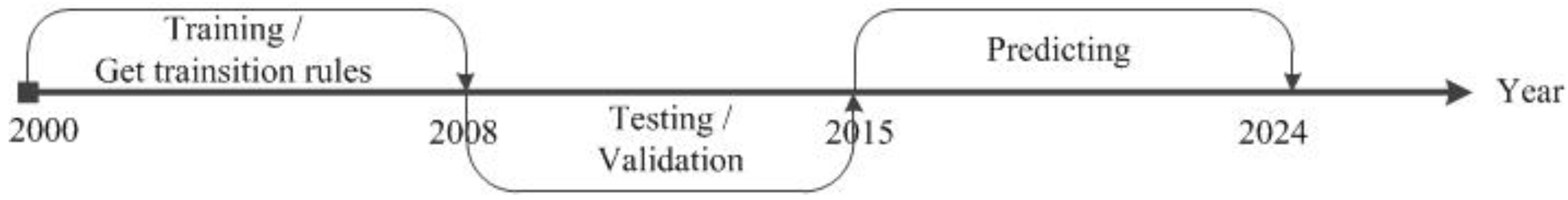
As shown in 
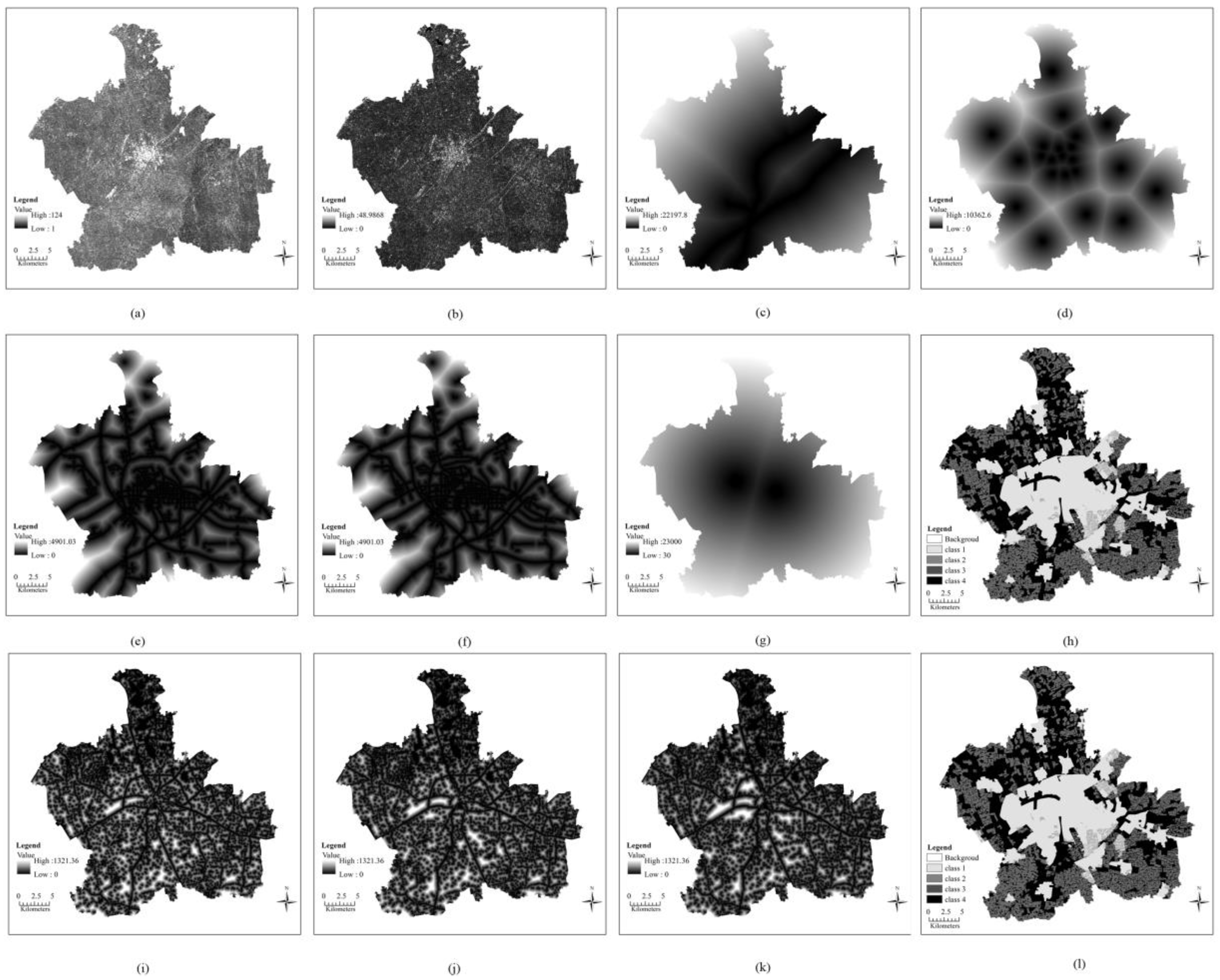
Figure 7, the initial year was 2000. Five thousand cells from 2000–2008 were selected by a stratified sampling method to serve as training data, while the ratio of developed/undeveloped cells in this sample was 2–3. Spatial variables including DEM, slope, Diswater, Disrailway, Disroad, Distown, Discounty, non-urban neighborhoods, urban neighborhoods and zoning suitability data were all used in the training, validation and prediction phases. Furthermore, the 2008–2015 validation process was used as an accuracy test, in which the majority of variables were calculated from the 2008 land use map and some from 2009; while in the 2015–2024 prediction phase, the 2015 land use map was considered as the fundamental image, in which zoning data were from 2015.
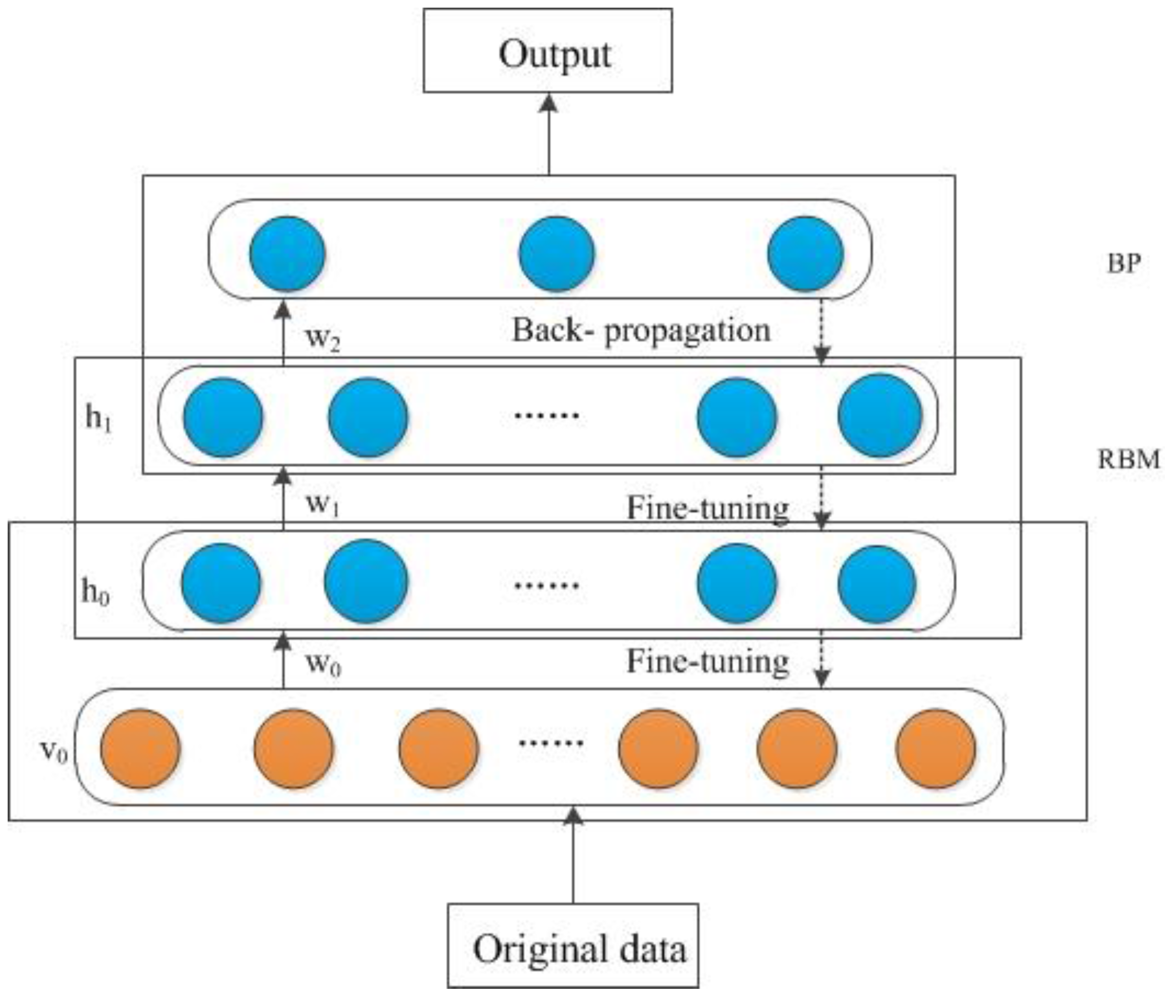
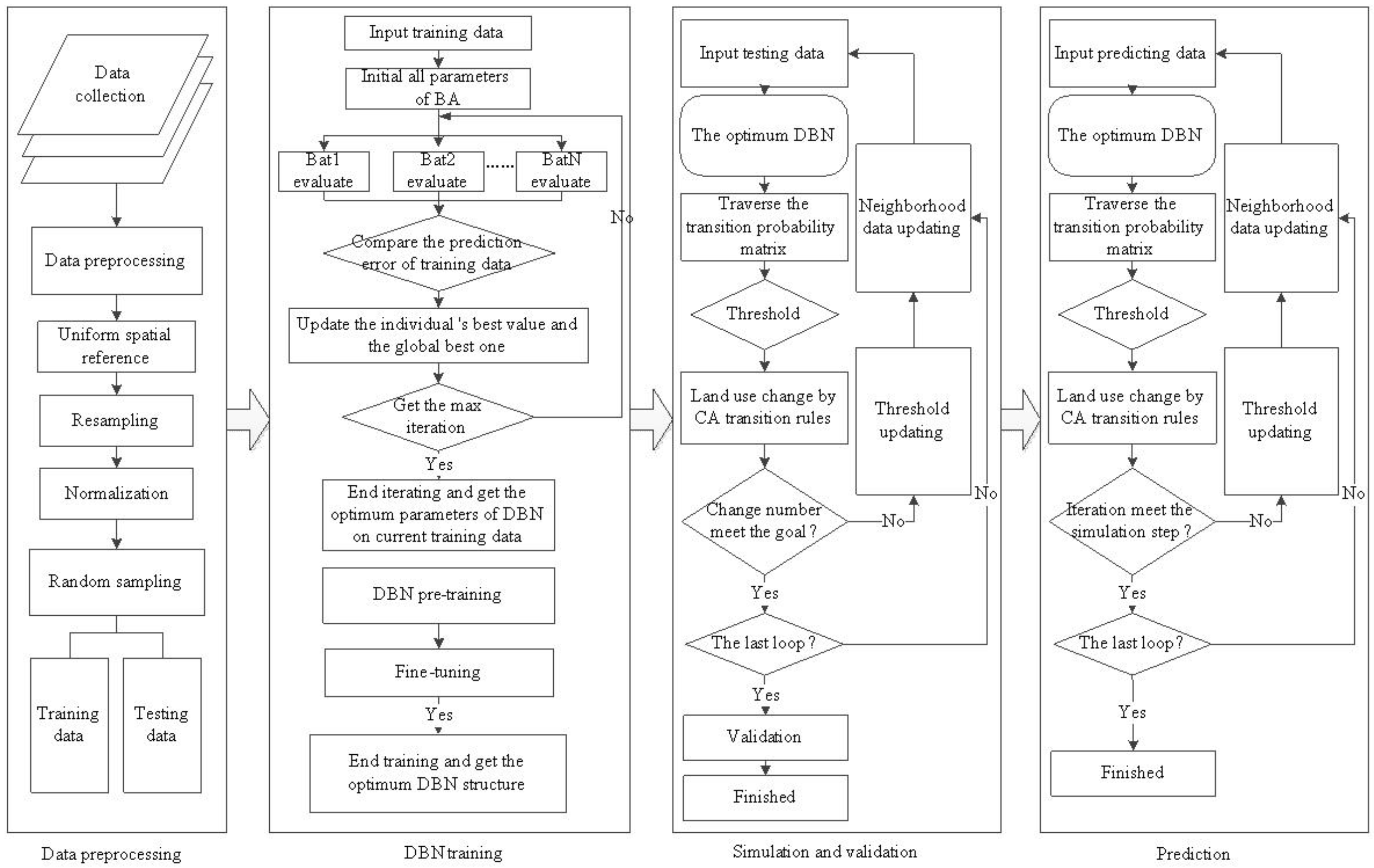
The architecture of the DBN-CA model is shown in Figure 3. First, the experimental data were converted to the same spatial reference (WGS_84_UTM_Zone_50N coordinate) and the same resolution (30 × 30 m). We performed experiments based on the DBN-CA model using the linear (Equation (7)) and the sigmoidal (Equation (8)) normalization methods, which normalized the data into [0,1] respectively:
x = x x m i n x m a x x m i n
x = 1 1 + exp ( x )
where x m i n is the minimum and x m a x is the maximum value of each variable. There were a total of 1,098,913 cells in the whole study area.
The simulation results of the experiments demonstrated that the linear normalization method is better than that of the sigmoidal normalization, since the linear normalization with a 78.366% kappa coefficient performs better than the sigmoidal one (with a 76.640% kappa coefficient). Therefore, the linear normalization method that is also commonly used in the literature [48,53] was adopted in this paper.
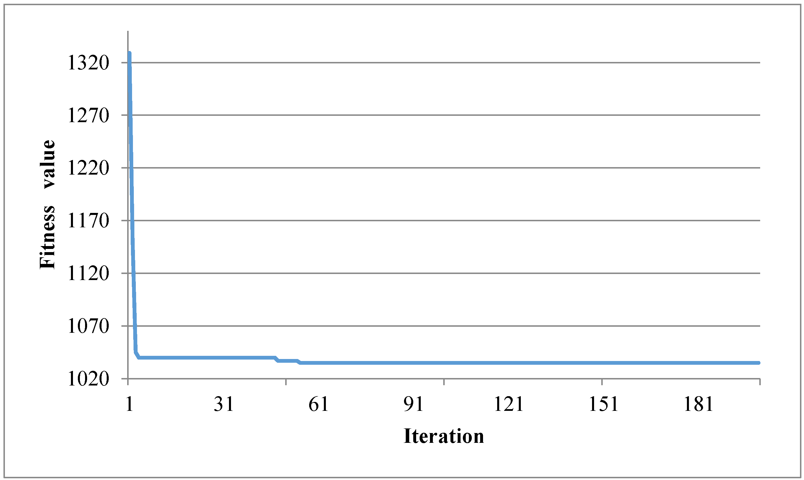
The second phase is DBN training, which aims to find the best DBN structure using the linear normalized training data. In this paper, we only discuss two RBM layers of DBN pre-training. The bat algorithm was performed to find the best architecture of DBN with training data. To implement the bat algorithm, we randomly initialized 40 bats (40 groups of RBM parameters, including the number of hidden units, learning rate, sparsity and dropout). The maximal and minimal pulse rates, loudness and frequency are 1 and 0, 2 and 1, 1.5 and 0, respectively. In addition, the fitness function (Equation (9)) can be calculated as the accumulated errors between the simulated probability and the observations of training data by DBN. The process was stopped when it reached 200 iterations.
f = i = 1 m j = 1 n ( p i j y i j ) 2
where m × n is the number of training data, p i j is 1 if the predicted probability by DBN is larger than the threshold, otherwise it is 0. y i j is the observation of the current cell. Otherwise, the learning rate of the fine-tuning phase was 0.01.
According to the above model parameters, we got the best fitness value of 1035 at the 55th iteration (Figure 8). The numbers of hidden units for the two RBM layers were 12 and 15; the learning rates were 0.016 and 0.069; and the sparsity and dropout were 0.0053 and 0.0016, respectively. Then, the DBN training module was used to obtain the optimum weights and bias of the CA parameters using RBM pre-training and BP fine-tuning. The DBN contains ten inputs (i.e., global variables and neighborhood variables mentioned before) and one output (one or zero, corresponding to non-urban developed into urban and non-urban undeveloped, respectively). The parameters of DBN were discussed in the BA module, and the number of iterations of each RBM was 50. The loop termination criterion considered both the maximum number of iterations and the accuracy of the model.
Third, the simulation and validation module was designed to obtain the transition probability matrix by predicting the testing data using the trained DBN, which was given in the DBN training module. In this research, we set the initial threshold p t h r e s h o l d at 0.8. The CA transition rules were defined as follows. First, the transition probability matrix was traversed to estimate if the transition probability p i j is bigger than p t h r e s h o l d and if the land use type changed from non-urban to urban in current cell ij. If it did not, it remained non-urban. Second, the neighborhood data were updated after each iteration, and the threshold was decreased by 0.002 if the total number of cells in the urban growth number was less than 100. The loop was repeated until the number of simulated urban units was almost identical to the observed data. Finally, a cell-by-cell comparison method was used to obtain the confusion matrix and kappa coefficient between the simulated map and the observed map, which was built to evaluate the result. In this paper, while calculating the kappa coefficient and confusion matrix, water was incorporated into the non-urban category.
The prediction phase was repeated as the third phase. It stopped once it reached the maximum iteration gained in the previous stage, and there was no validation.
The ANN and DBN training module and all the models’ simulation and validation were implemented using MATLAB software.

4.2. Analysis of the Observed Data

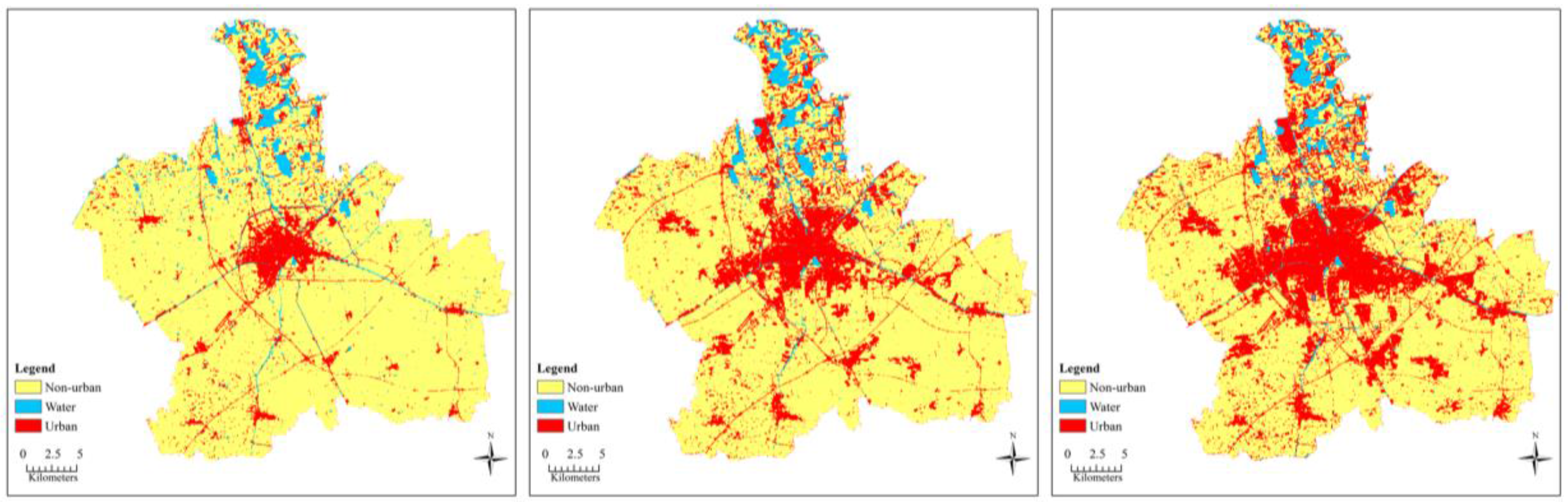
Tremendous non-urban areas were converted into urban areas between 2000 and 2015. Concurrently, water was relatively stable. Table 2 summarizes the land use type cells, percentages, gains and losses for the three time periods in Jiaxing City: 2000–2008, 2008–2015 and 2000–2015. In the period from 2000–2008, 106,014 non-urban cells (equivalent to 9541.26 ha, 9.647% of the total number of cells) and 1668 cells (equivalent to 150.12 hectares, 0.151% of the total number of cells) of water were transformed to urban use. Urban land increased by 8.845% (8747.73 hectares) from 2008 –2015. Jiaxing City rapidly developed between 2000 and 2015, as the urban land increased by 18.643% of the total number of cells, and almost all of them (17,975.61 hectares) were derived from non-urban cells.

4.3. A Comparison of the Simulation Results between DBN-CA and ANN-CA

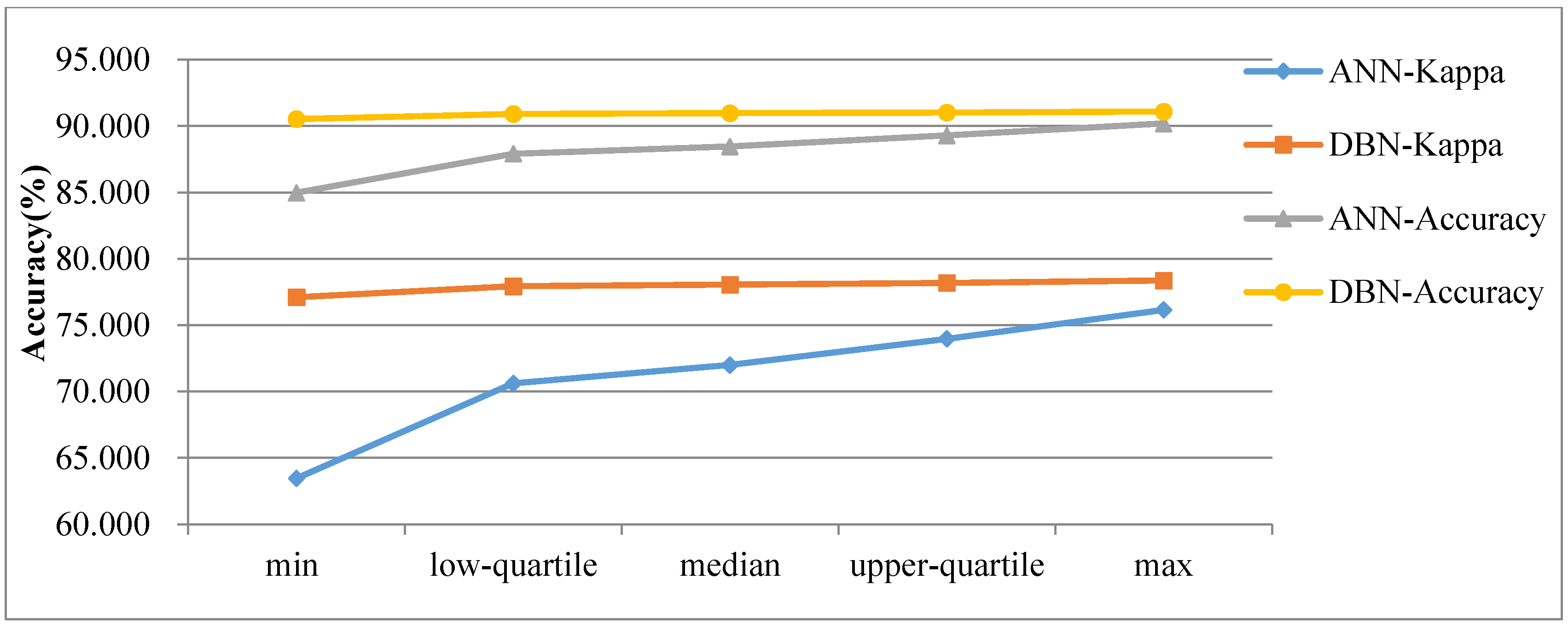
To reduce the error caused by random initialization in the weights and biases of ANN, we repeated the process 200 times to test the ANN-CA. Additionally, after obtaining the optimum structure of DBN using BA, we conducted 200 tests on the DBN-CA. Exploratory data analysis methods were used to explore the five-number summary of the ANN-CA and DBN-CA simulation results, including the minimum, maximum, median, upper quartile and lower quartile values of the kappa coefficient and overall accuracy of these two models over the 200 experiments (Figure 9). The minimum kappa coefficient of the DBN-CA and ANN-CA was 63.460% and 77.109%, respectively, while the maximum of the DBN-CA was 78.366%, almost 2.215% larger than the value for the ANN-CA. The lower-quartile, median and upper-quartile kappa coefficient of the proposed model and compared model were 77.931%, 78.050% and 78.187% and 70.610%, 72.001% and 73.966%, respectively. The overall accuracy values from the five-number summary of the DBN-CA and ANN-CA were 90.533%, 90.916%, 90.971%, 91.019% and 91.100% and 84.971%, 87.913%, 88.457%, 89.294% and 90.191%, respectively.
From the data summarized in Figure 9, we see that the simulation results of the proposed model are much more stable than those obtained using the ANN-CA model, since the difference between the minimum and maximum values of overall accuracy and kappa coefficient were 0.567% and 1.257%, while the ANN-CA’s values were 5.220% and 12.691%, respectively. Furthermore, the DBN-CA model has, on average, a higher accuracy and kappa coefficient than the ANN-CA.
We have performed a general analysis of the 200 tests’ simulation results for the DBN-CA and ANN-CA models using the five-number summary approach above. Next, we chose the best results of these two models to compare and analyze.
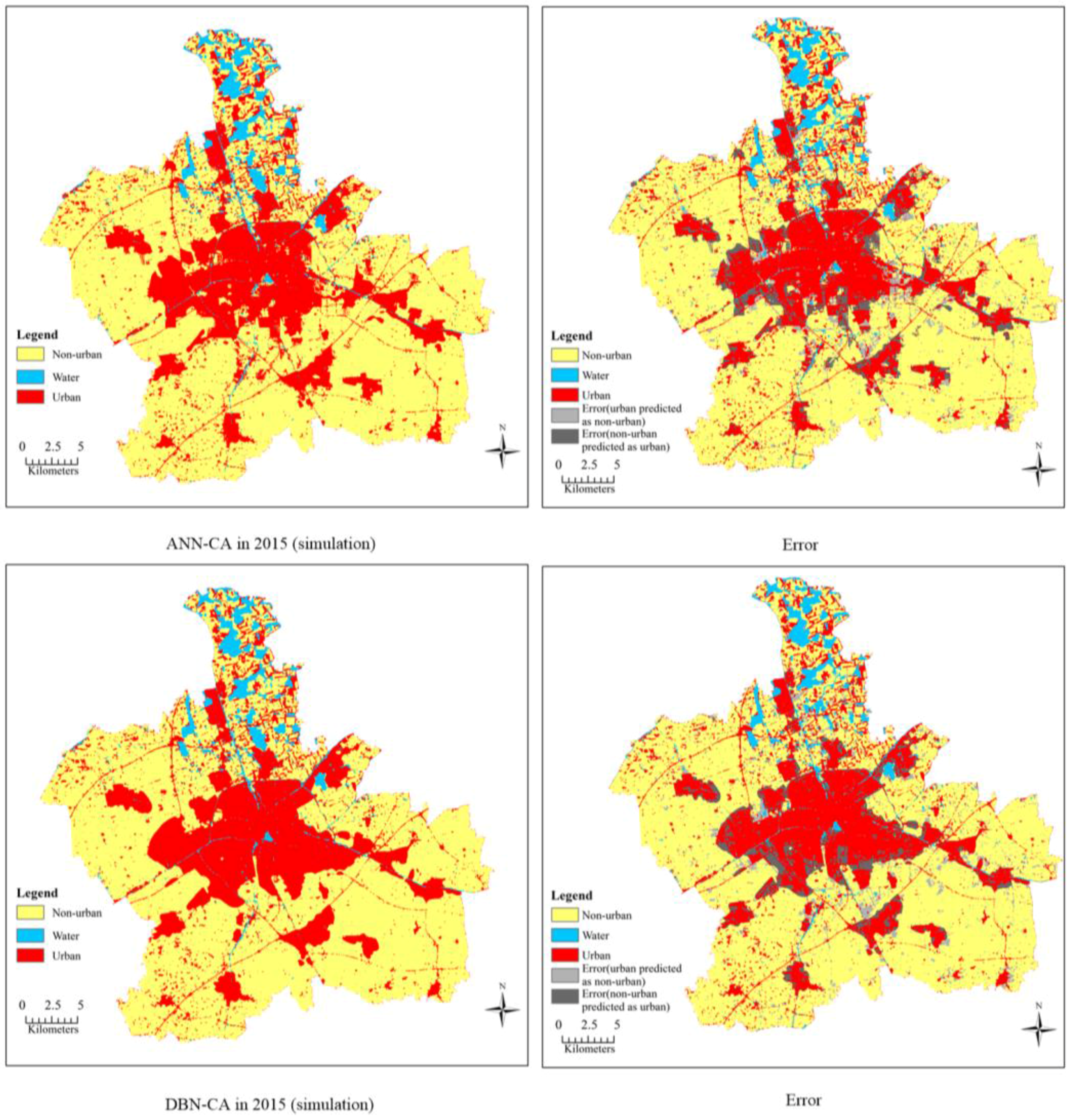
Table 3 summarizes the simulated data on land use types obtained using the DBN-CA and ANN-CA models for the research area in 2015. Compared with the observed datasets, the simulation errors compared with the observed values for the non-urban, water and urban areas using the DBN-CA model were 0.564%, 7.663% and 0.209%, respectively, while the errors of the ANN-CA model simulation results were 0.523%, 7.663% and 0.115%, respectively. For the whole study area, we obtained the average error of 2.812% in the DBN-CA and 2.767% in the ANN-CA model respectively, which were acceptable. However, we need further analysis since the high precision of the whole area might not lead to the high simulation accuracy of the models due to contingencies.
Figure 10 provides the best simulation maps and error maps of the DBN-CA and ANN-CA over 200 trails. The two models’ simulation results showed a consistent trend of expansion from the city center to outlying areas. The dense population at the city center and its convenient transportation directly led to the rapid expansion of the downtown area from 2000–2015.
Furthermore, the confusion matrix tables between the simulated results and the observed data permit us to evaluate the precision of the DBN-CA and ANN-CA models (Table 4 and Table 5). In the DBN-CA model, the correct simulated number of non-urban areas (including water) reaches 731,808 cells, while the urban land area reaches 269,292 cells. Table 4 shows that the correct simulated numbers of non-urban (including water) and urban areas are 726,966 cells and 264,151 cells, respectively, which were observed in the ANN-CA model. In addition, the simulation results were good for the ANN-CA and DBN-CA since the kappa coefficients for these two models were greater than 75% and the overall accuracies were higher than 90%. However, the DBN-CA with a 78.366% kappa coefficient performed much better on the urban expansion simulation than the ANN-CA with a 76.151% kappa coefficient since the kappa coefficient was 2.215% higher.
Rapid urban expansion has brought a series of ecological and resource problems to the study area, so an effective approach to simulate urban growth can provide strong support for ecological protection and urban planning. Although the DBN-CA cannot perfectly reproduce the real world, it has been shown that DBN is more capable and stable in mining the transition rules than the ANN in Jiaxing City during 2000–2015.

4.4. Prediction

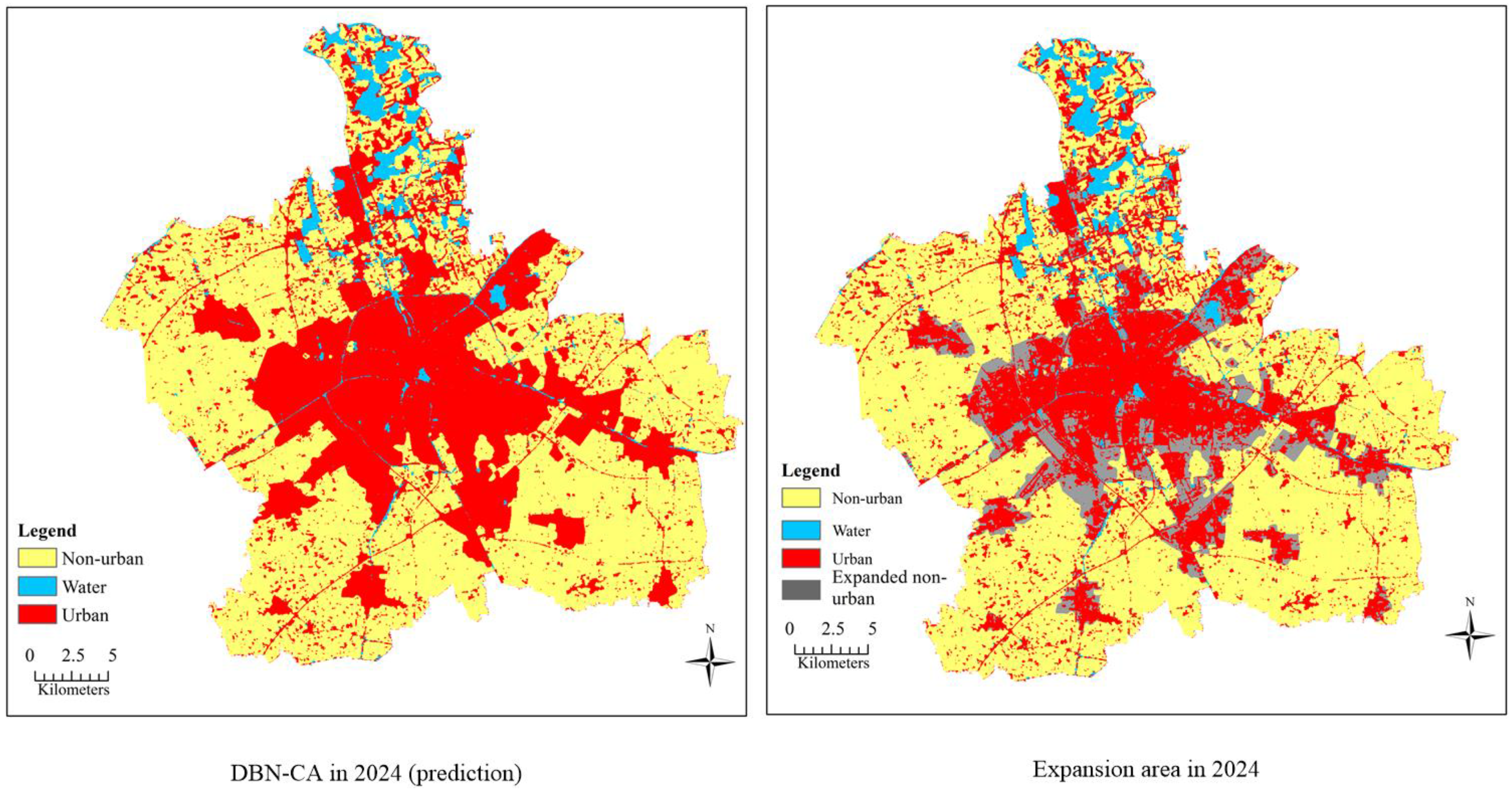
After simulation and validation, in order to estimate the non-urban loss during urbanization in the next decade, we predicted urban expansion for the year 2024. As we demonstrated that the DBN-CA model was more stable and had better performance than the ANN-CA model in 2015, it was used to simulate urban expansion based on the 2015 land use map and other global or constraint variables, as well as the 7 × 7 window Moore neighborhoods. Figure 11 shows the potential non-urban areas that were more likely to be converted into urban land in 2024. According to the statistics, there will be almost 8946.36 hectares (13.513%) of non-urban land that may be lost over the next ten years, and these are located along the border of each town. The results also showed the outward expansion trend of Jiaxing City.

5. Conclusions

This paper made a brief quantitative analysis of non-urban land conversion of Jiaxing City in Zhejiang Province from 2000–2015. The historical data showed that 18.175% of the non-urban land was converted to urban areas, and the urban areas had increased from 10.282%–28.925%. Furthermore, an integrated model by associating the bat algorithm, the deep belief network, cellular automata and GIS was developed to model non-urban land use changes and understand the processes of urban growth. The DBN-CA model framework was proposed, which included spatial data processing, DBN training, urban growth simulation, validation and effective prediction. The DBN-CA model framework with high simulation precision and strong self-adaptive ability was built for the public.
This paper obtained the urban growth transition rules from 2000–2008 in Jiaxing City based on the bat algorithm, unsupervised learning (pre-training) and the supervised learning (BP fine-tuning) of DBN. Land use from 2008–2015 was used to simulate and validate the optimum DBN structure. To reduce the random error of the models, 200 iterations of the DBN-CA and ANN-CA model simulations were conducted. The five-number summary of the simulation overall accuracy and kappa coefficient showed that the DBN-CA model was much more stable than the ANN-CA model. Analyzing the best results of these two models, the kappa coefficients are all greater than 75%, but the one for the DBN-CA model is 2.215% higher than that for the ANN-CA model. This demonstrates that DBN-CA and ANN-CA are both able to simulate complex and nonlinear urban growth. This also demonstrated that the DBN-CA is a new promising approach to simulate urban growth due to its higher simulation accuracy and stability. Finally, according to the prediction of urban growth of Jiaxing City for 2024, it will still present an expansion trend for towns. The predicted land use map indicated that 8946.36 hectares of non-urban areas will be converted to urban areas in 2015.
The proposed model used to simulate the urban growth in the example of Jiaxing City led to a new and effective land use change and urban expansion simulation approach. The DBN-CA model can be considered as a useful tool for urban planning and its related personnel, ecologists and resource managers who are committed to sustainable development. However, the bat algorithm requires more than 10 hours to optimize the DBN for 40 bats and 200 iterations on a personal computer with a 3.60-GHz CPU and 8 GB RAM. Therefore, a future study direction may be to investigate methods of improving the calculation speed. Moreover, as the “non-urban” category in this paper is very widely defined, a more refined classification would enable us to understand which type of land is more suitable to develop into urban land.

Acknowledgments

This work was supported by the National Natural Science Foundation of China (41471313, 41671391), the Science and Technology Project of Zhejiang Province (2014C33G20), the Public Science and Technology Research Funds’ Projects (2015418003) and the National Science Foundation ACI-1535031, 1535081.

Author Contributions

Ye Zhou contributed to the algorithm improvement and drafted the manuscript. Feng Zhang conceived of and designed the study and also provided the funding. Zhenhong Du was involved in data acquisition and analysis and worked on aspects of the experiment evaluation. Xinyue Ye improved the conceptual framework and updated the manuscript. Renyi Liu was involved in the study design and revision of the manuscript and drafted the manuscript. All authors have read and approved the final manuscript.

Conflicts of Interest

The authors declare no conflict of interest.

References

  1. Dale, V.H.; O'Neill, R.V.; Pedlowski, M.; Southworth, F. Causes and effects of land-use change in central Rondonia, Brazil. Photogramm. Eng. Remote Sens. 1993, 59, 997–1005. [Google Scholar]
  2. Pijanowski, B.C.; Brown, D.G.; Shellito, B.A.; Manik, G.A. Using neural networks and GIS to forecast land use changes: a Land Transformation Model. Comput. Environ. Urban Syst. 2002, 26, 553–575. [Google Scholar] [CrossRef]
  3. Xu, Y.; Mcnamara, P.; Wu, Y.; Dong, Y. An econometric analysis of changes in arable land utilization using multinomial logit model in Pinggu district, Beijing, China. J. Enviorn. Manag. 2013, 128, 324. [Google Scholar] [CrossRef] [PubMed]
  4. Li, H.; Wei, Y.H.D.; Huang, Z.J. Urban land expansion and spatial dynamics in globalizing Shanghai. Sustainability 2014, 6, 8856–8875. [Google Scholar] [CrossRef]
  5. Rasmussen, L.V.; Rasmussen, K.; Reenberg, A.; Proud, S. A system dynamics approach to land use changes in agro-pastoral systems on the desert margins of Sahel. Agric. Syst. 2012, 107, 56–64. [Google Scholar] [CrossRef]
  6. Clark, A.S. The political institutional determinants of land-use change and sprawl: a conceptual model. Theor. Empir. Res. Urban Manag. 2010, 5, 5–18. [Google Scholar]
  7. Muller, M.R.; Middleton, J. A Markov model of land-use change dynamics in the Niagara Region, Ontario, Canada. Landsc. Ecol. 1994, 9, 151–157. [Google Scholar]
  8. Li, X.; Li, X.; Peng, W.; Tong, C. Modelling urban sprawl with the optimal integration of Markov chain and spatial neighborhood analysis approach. Geosci. Remote Sens. Symp. 2004, 4, 2658–2661. [Google Scholar]
  9. Ralha, C.G.; Abreu, C.G.; Coelho, C.G.C.; Zaghetto, A.; Macchiavello, B.; Machado, R.B. A multi-agent model system for land-use change simulation. Environ. Modell. Softw. 2013, 42, 30–46. [Google Scholar] [CrossRef]
  10. Liu, D.; Zheng, X.; Zhang, C.; Wang, H. A new temporal–spatial dynamics method of simulating land-use change. Ecol. Model. 2017, 350, 1–10. [Google Scholar] [CrossRef]
  11. Losiri, C.; Nagai, M.; Ninsawat, S. Modeling Urban Expansion in Bangkok Metropolitan Region Using Demographic–Economic Data through Cellular Automata-Markov Chain and Multi-Layer Perceptron-Markov Chain Models. Sustainability 2016, 8, 686. [Google Scholar] [CrossRef]
  12. García, A.M.; Santé, I.; Boullón, M.; Crecente, R. Calibration of an urban cellular automaton model by using statistical techniques and a genetic algorithm. Application to a small urban settlement of NW Spain. Int. J. Geogr. Inf. Sci. 2013, 27, 1593–1611. [Google Scholar] [CrossRef]
  13. Ke, X.; Qi, L.; Zeng, C. A partitioned and asynchronous cellular automata model for urban growth simulation. Int. J. Geogr. Inf. Sci. 2016, 30, 1–23. [Google Scholar] [CrossRef]
  14. Tobler, W.R. A computer movie simulating urban growth in the Detroit region. Geogr. Econ. 1970, 46, 234–240. [Google Scholar] [CrossRef]
  15. White, R.; Engelen, G. Cellular automata and fractal urban form: a cellular modelling approach to the evolution of urban land-use patterns. Environ. Plan. A 1993, 25, 1175–1199. [Google Scholar] [CrossRef]
  16. Clarke, K.C.; Hoppen, S.; Gaydos, L. A self-modifying cellular automaton model of historical urbanization in the San Francisco Bay area. Environ. Plan. B Plan. Des. 1997, 24, 247–261. [Google Scholar] [CrossRef]
  17. Clarke, K.C.; Gaydos, L.J. Loose-coupling a cellular automaton model and GIS: long-term urban growth prediction for San Francisco and Washington/Baltimore. Int. J. Geogr. Inf. Sci. 1998, 12, 699–714. [Google Scholar] [CrossRef] [PubMed]
  18. Li, X.; Yeh, G.O. Neural-network-based cellular automata for simulating multiple land use changes using GIS. Int. J. Geogr. Inf. Sci. 2002, 16, 323–343. [Google Scholar] [CrossRef]
  19. Almeida, C.M.; Gleriani, J.M.; Castejon, E.F.; Soares-Filho, B.S. Using neural networks and cellular automata for modeling intra-urban land-use dynamics. Int. J. Geogr. Inf. Sci. 2008, 22, 943–963. [Google Scholar] [CrossRef]
  20. Liao, J.; Tang, L.; Shao, G.; Qiu, Q.; Wang, C.; Zheng, S. A neighbor decay cellular automata approach for simulating urban expansion based on particle swarm intelligence. Int. J. Geogr. Inf. Sci. 2014, 28, 720–738. [Google Scholar] [CrossRef]
  21. Basse, R.M.; Omrani, H.; Charif, O.; Gerber, P.; Bódis, K. Land use changes modelling using advanced methods: Cellular automata and artificial neural networks. The spatial and explicit representation of land cover dynamics at the cross-border region scale. Appl. Geogr. 2014, 53, 160–171. [Google Scholar] [CrossRef]
  22. Cao, K.; Huang, B.; Li, M.; Li, W. Calibrating a cellular automata model for understanding rural-urban land conversion: a Pareto front-based multi-objective optimization approach. Int. J. Geogr. Inf. Sci. 2014, 28, 1028–1046. [Google Scholar] [CrossRef]
  23. Azari, M.; Tayyebi, A.; Helbich, M.; Reveshty, M.A. Integrating cellular automata, artificial neural network, and fuzzy set theory to simulate threatened orchards: application to Maragheh, Iran. Gisci. Remote Sens. 2016, 53, 183–205. [Google Scholar] [CrossRef]
  24. Wu, F. Calibration of stochastic cellular automata: the application to rural-urban land conversions. Int. J. Geogr. Inf. Sci. 2002, 16, 795–818. [Google Scholar] [CrossRef]
  25. Silva, E.A.; Clarke, K.C. Complexity, emergence and cellular urban models: lessons learned from applying SLEUTH to two Portuguese metropolitan areas. Eur. Plan. Stu. 2005, 13, 93–115. [Google Scholar] [CrossRef]
  26. Rienow, A.; Goetzke, R. Supporting SLEUTH—Enhancing a cellular automaton with support vector machines for urban growth modeling. Comput. Environ. Urban Syst. 2015, 49, 66–81. [Google Scholar] [CrossRef]
  27. Wu, F. SimLand: a prototype to simulate land conversion through the integrated GIS and CA with AHP-derived transition rules. Int. J. Geogr. Inf. Sci. 1998, 12, 63–82. [Google Scholar] [CrossRef]
  28. Wu, F.; Webster, C.J. Simulation of land development through the integration of cellular automata and multicriteria evaluation. Environ. Plan. B Plan. Des. 1998, 25, 103–126. [Google Scholar] [CrossRef]
  29. Poelmans, L.; Rompaey, A.V. Complexity and performance of urban expansion models. Comput. Environ. Urban Syst. 2010, 34, 17–27. [Google Scholar] [CrossRef]
  30. Munshi, T.; Zuidgeest, M.; Brussel, M.; Maarseveen, M.V. Logistic regression and cellular automata-based modelling of retail, commercial and residential development in the city of Ahmedabad, India. Cities 2014, 39, 68–86. [Google Scholar] [CrossRef]
  31. Cao, M.; Bennett, S.J.; Shen, Q.; Xu, R. A bat-inspired approach to define transition rules for a cellular automaton model used to simulate urban expansion. Int. J. Geogr. Inf. Sci. 2016, 30, 1–19. [Google Scholar] [CrossRef]
  32. Li, X.; Lin, J.; Chen, Y.; Liu, X.; Ai, B. Calibrating cellular automata based on landscape metrics by using genetic algorithms. Int. J. Geogr. Inf. Sci. 2013, 27, 594–613. [Google Scholar] [CrossRef]
  33. Liu, X.; Li, X.; Liu, L.; He, J.; Ai, B. A bottom-up approach to discover transition rules of cellular automata using ant intelligence. Int. J. Geogr. Inf. Sci. 2008, 22, 1247–1269. [Google Scholar] [CrossRef]
  34. Tayyebi, A.; Pijanowski, B.C.; Tayyebi, A.H. An urban growth boundary model using neural networks, GIS and radial parameterization: An application to Tehran, Iran. Landsc. Urban Plan. 2011, 100, 35–44. [Google Scholar] [CrossRef]
  35. Hinton, G.E.; Osindero, S.; Teh, Y.W. A fast learning algorithm for deep belief nets. Neural Comput. 2006, 18, 1527–1554. [Google Scholar] [CrossRef] [PubMed]
  36. Dahl, G.E.; Yu, D.; Deng, L.; Acero, A. Context-dependent pre-trained deep neural networks for large-vocabulary speech recognition. Trance. Audio. Speech Lang. Process. 2011, 20, 30–42. [Google Scholar] [CrossRef]
  37. Yu, D.; Seltzer, M.L.; Li, J.; Huang, J.T.; Seide, F. Feature Learning in Deep Neural Networks—Studies on Speech Recognition Tasks. Available online: http://arxiv.org/pdf/1301.3605 (accessed on 2 October 2016).
  38. Shen, F.; Chao, J.; Zhao, J. Forecasting exchange rate using deep belief networks and conjugate gradient method. Neural Comput. 2015, 167, 243–253. [Google Scholar] [CrossRef]
  39. Hinton, G.E. Learning multiple layers of representation. Trends. Cogn. Sci. 2007, 11, 428–434. [Google Scholar] [CrossRef] [PubMed]
  40. Wei, Q.; Li, H.; Zhou, X. The Appropriate Hidden Layers of Deep Belief Networks for Speech Recognition; Intelligent Systems and Knowledge Engineering (ISKE): Taipei, Taiwan, 2015. [Google Scholar]
  41. Grekousis, G.; Manetos, P.; Photis, Y.N. Modeling urban evolution using neural networks, fuzzy logic and GIS: The case of the Athens metropolitan area. Cities 2013, 30, 193–203. [Google Scholar] [CrossRef]
  42. Mahboob, M.A.; Atif, I.; Iqbal, J. Remote sensing and GIS applications for assessment of urban sprawl in Karachi, Pakistan. Sci. Technol. Dev. 2015, 34, 179–188. [Google Scholar] [CrossRef]
  43. Alsharif, A.A.; Pradhan, B. Urban sprawl analysis of Tripoli Metropolitan City (Libya) using remote sensing data and multivariate logistic regression model. J. Indian Soc. Remote. 2014, 42, 149–163. [Google Scholar] [CrossRef]
  44. Triantakonstantis, D.; Stathakis, D. Urban growth prediction in Athens, Greece, using Artificial Neural Networks. Int. J. Civ. Environ. Struct. Constr. Archit. Eng. 2015, 9, 234–238. [Google Scholar]
  45. Kazemzadeh-zow, A.; Shahraki, S.Z.; Salvati, L.; Samani, N.N. A spatial zoning approach to calibrate and validate urban growth models. Int. J. Geogr. Inf. Sci. 2017, 31, 763–782. [Google Scholar] [CrossRef]
  46. Riccioli, F.; El Asmar, T.; El Asmar, J.-P.; Fagarazzi, C.; Casini, L. Artificial neural network for multifunctional areas. Environ. Monit. Assess. 2016, 188, 67. [Google Scholar] [CrossRef] [PubMed]
  47. Berberoğlu, S.; Akın, A.; Clarke, K.C. Cellular automata modeling approaches to forecast urban growth for adana, Turkey: A comparative approach. Landsc. Urban Plan. 2016, 153, 11–27. [Google Scholar]
  48. Riccioli, F.; El Asmar, T.; El Asmar, J.-P.; Fratini, R. Use of cellular automata in the study of variables involved in land use changes: an application in the wine production sector. Environ. Monit. Assess. 2013, 185, 5361–5374. [Google Scholar] [CrossRef] [PubMed]
  49. Yang, X.S. A new metaheuristic bat-inspired algorithm. Comput. Knowl. Technol. 2010, 284, 65–74. [Google Scholar]
  50. Von Neumann, J. Theory of Self-Reproducing Automata; Burks, A.W., Ed.; University of Illinois Press: Urbana, IL, USA; London, UK, 1966. [Google Scholar]
  51. Hinton, G.E. Training products of experts by minimizing contrastive divergence. Neural Comput. 2002, 14, 1771–1800. [Google Scholar] [CrossRef] [PubMed]
  52. Batty, M.; Xie, Y. From Cells to Cities. Environ. Plan. B Plan. Des. 1994, 21, 31. [Google Scholar] [CrossRef]
  53. Cao, M.; Tang, G.; Shen, Q.F.; Wang, Y.X. A new discovery of transition rules for cellular automata by using cuckoo search algorithm. Int. J. Geogr. Inf. Sci. 2015, 29, 806–824. [Google Scholar] [CrossRef]
Figure 1. Architecture of the deep belief network (DBN).
Sustainability 09 01786 g001
Figure 2. Architecture of the restricted Boltzmann machine (RBM).
Sustainability 09 01786 g002
Figure 3. The architecture of the DBN-cellular automata (CA) model. BA, bat algorithm.
Sustainability 09 01786 g003
Figure 4. Location of Jiaxing City, Zhejiang Province.
Sustainability 09 01786 g004
Figure 5. Land use maps of Jiaxing City in 2000, 2008 and 2015.
Sustainability 09 01786 g005
Figure 6. Global factors: (a) DEM, (b) slope, (c) Disrailway, (d) Distown, (e) Disroad2008, (f) Disroad2016, (g) Discounty, (h) Zoning2009, (i) Diswater2000, (j) Diswater2008, (k) Diswater2015, (l) Zoning2015.
Sustainability 09 01786 g006
Figure 7. Model processing.
Sustainability 09 01786 g007
Figure 8. The convergence of the fitness value in the BA process.
Sustainability 09 01786 g008
Figure 9. Data feature description of ANN-CA and DBN-CA.
Sustainability 09 01786 g009
Figure 10. Simulation and error results of DBN-CA and ANN-CA in 2015.
Sustainability 09 01786 g010
Figure 11. Prediction of non-urban conversion to urban obtained by DBN-CA in 2024.
Sustainability 09 01786 g011
Table 1. Summary of the ANN-CA and DBN-CA model inputs.
VariablesDescription
YDependent variable, designated as 0 if the state of a non-urban cell is unchanged or 1 if a non-urban cell developed into an urban cell
DEM/SlopeThe DEM and slope of Jiaxing City
DiswaterEuclidean distance from the cell to the nearest river calculated from land use maps in 2000, 2008 and 2015
DisrailwayEuclidean distance from the cell to the nearest railway
DisroadEuclidean distance from the cell to the nearest road in 2008 and 2016
DistownEuclidean distance from the cell to the nearest town center
DiscountyEuclidean distance from the cell to the nearest county center
Non-urban neighborhoodsNumber of non-urban cells in the 7 × 7 extended Moore neighborhood at different times
Urban neighborhoodsNumber of non-urban cells in the 7 × 7 extended Moore neighborhood at different times
Zoning suitabilityClasses from land use planning and high quality prime farmland data in 2009 and 2015
Table 2. Land use change in the 2000–2008, 2008–2015 and 2000–2015 periods.
Land Use TypeTotal DatasetGain and Loss
2000200820152000–20082008–20152000–2015
Non-urban#935,339829,325735,610−106,014−93,715−199,729
ha84,180.5174,639.2566,204.9−9541.26−8434.35−17,975.61
%85.11575.46866.94−9.647−8.528−18.175
Water#50,58748,91945,437−1668−3482−5150
ha4552.834402.714089.33−150.12−313.38−463.5
%4.6034.4524.135−0.151−0.317−0.468
Urban#112,987220,669317,866107,68297,197204,879
ha10,168.8319,860.2128,607.949691.388747.7318,439.11
%10.28220.0828.9259.7988.84518.643
total#1,098,9131,098,9131,098,913000
ha98,902.1798,902.1798,902.17000
%100100100000
Abbreviations: # means the number of cells, ha is hectares and % means percent.
Table 3. Simulation land use change by DBN-CA and ANN-CA.
Land Use Type2015 (Cell)
ObservedSimulated by ANN-CAErrorSimulated by DBN-CAError
Non-urban735,610731,762−3848731,463−4147
Water45,43748,919348248,9193482
Urban317,866318,232366318,531665
Sum1,098,9131,098,91301,098,9130
Table 4. Confusion matrix between ANN-CA simulated result and the observed data.
ANN-CA Simulated land Use in 2015 (Cells)Simulation Accuracy (%)
Observed land use in 2015non-urbanurbanProducer’s accuracyUser’s accuracyOverall accuracyKappa coefficient
726,96654,08193.07693.11990.19176.151
53,715264,15183.10183.006
Table 5. Confusion matrix between the DBN-CA simulated result and the observed data.
DBN-CA Simulated Land Use in 2015 (Cells)Simulation Accuracy (%)
Observed land use in 2015non-urbanurbanProducer’s accuracyUser’s accuracyOverall accuracyKappa coefficient
731,80849,23993.69693.77691.09978.366
48,574269,29284.71984.542

