
Exploring the Effects of Sampling Locations for Calibrating the Huff Model Using Mobile Phone Location Data


Abstract
:1. Introduction
- (1)
- Does using all sampling locations always perform better than small volume of sampling locations to calibrate the Huff model?
- (2)
- If not, what kinds of sampling locations are more effective for calibrating this model?
2. Study Area and Dataset
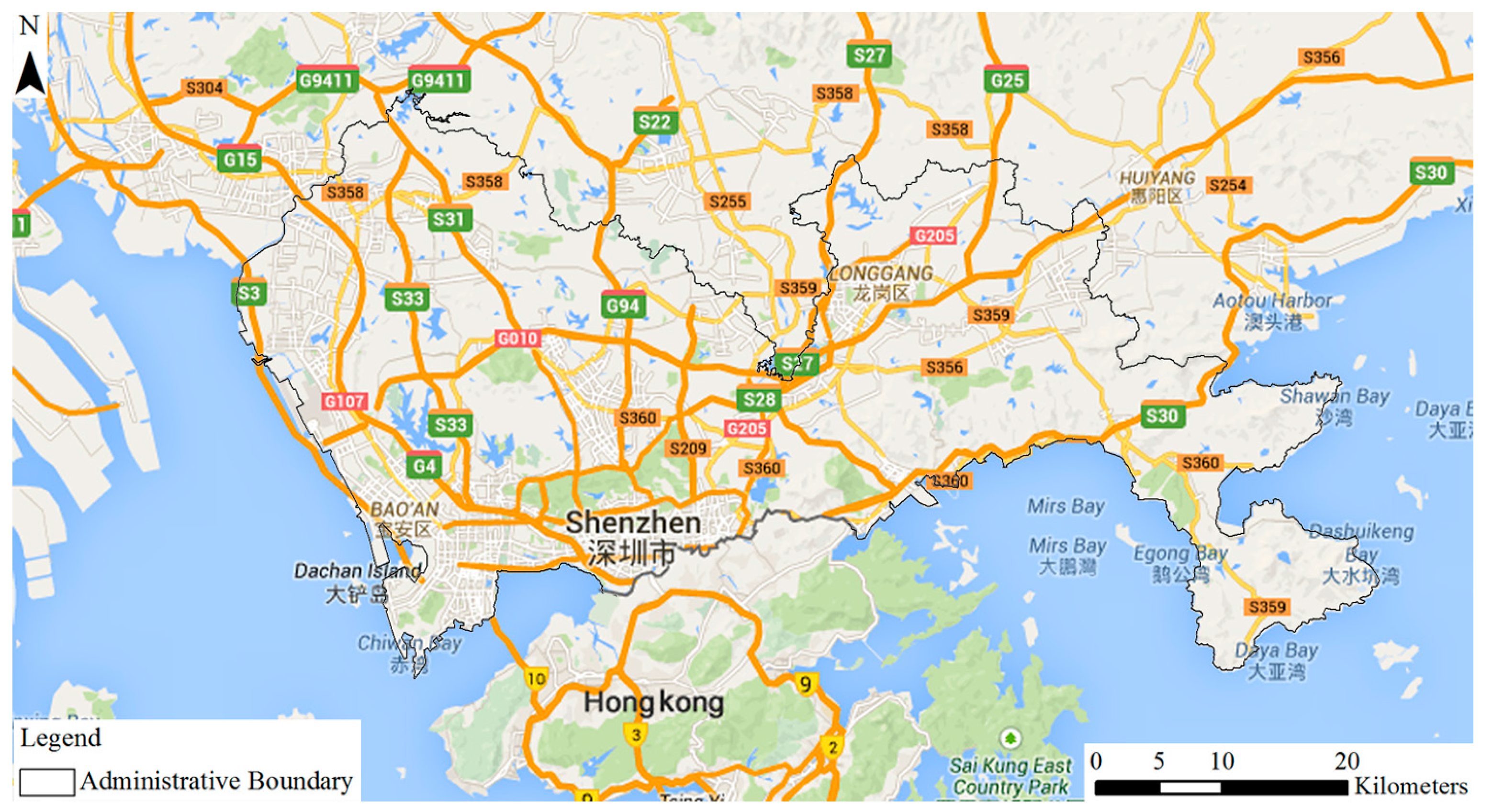
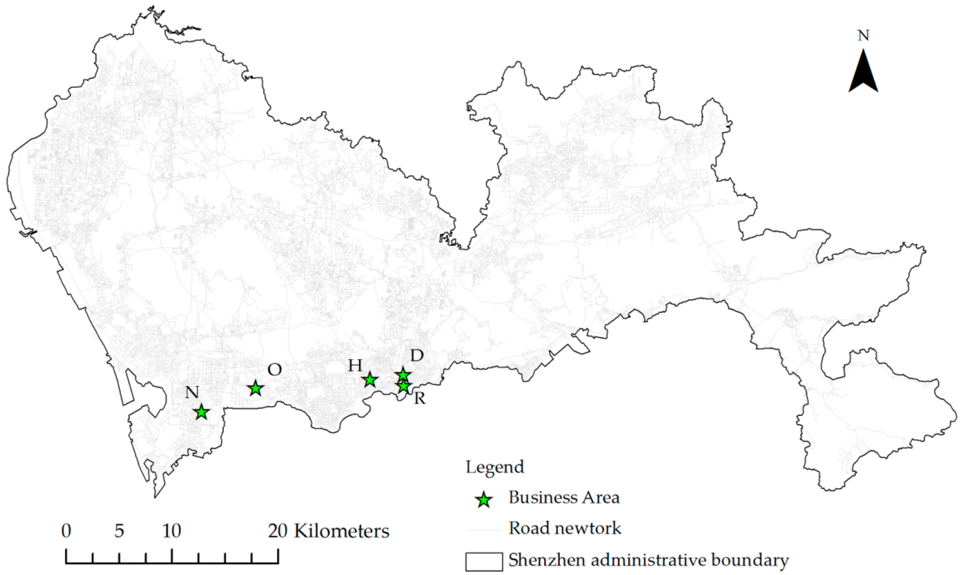
2.1. Study Area
2.2. Data Description
3. Methodology
3.1. Extracting Trips towards Commercial Areas
- Rule 1:
- Stay duration is no less than 1 h
- Rule 2:
- The arrival time is after 9:00 a.m.
- Rule 3:
- The leave time is before 11:00 p.m.
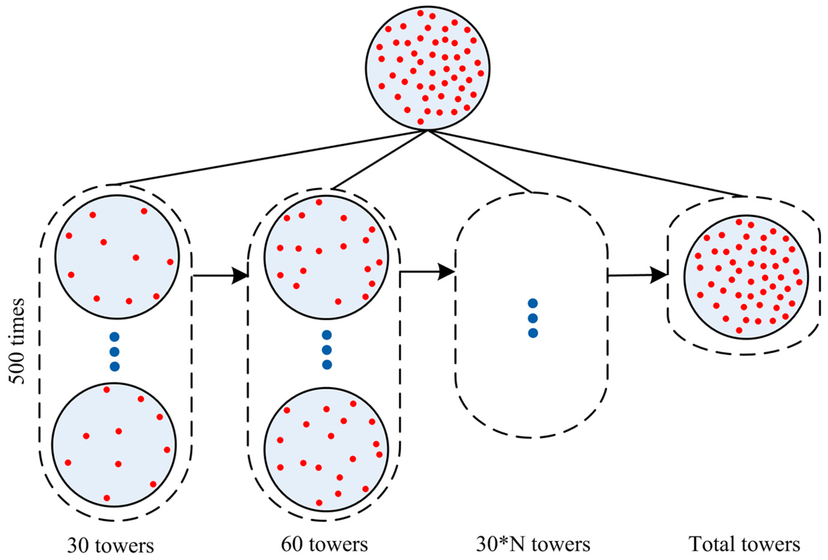
3.2. Randomly Calibrate the Huff Model
4. Results
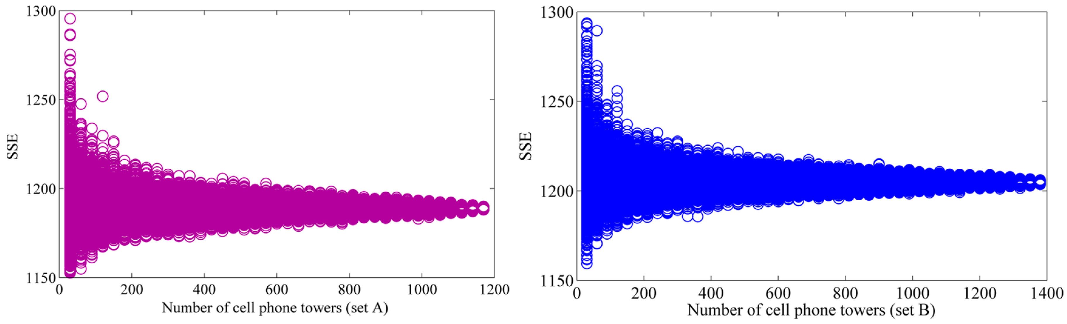
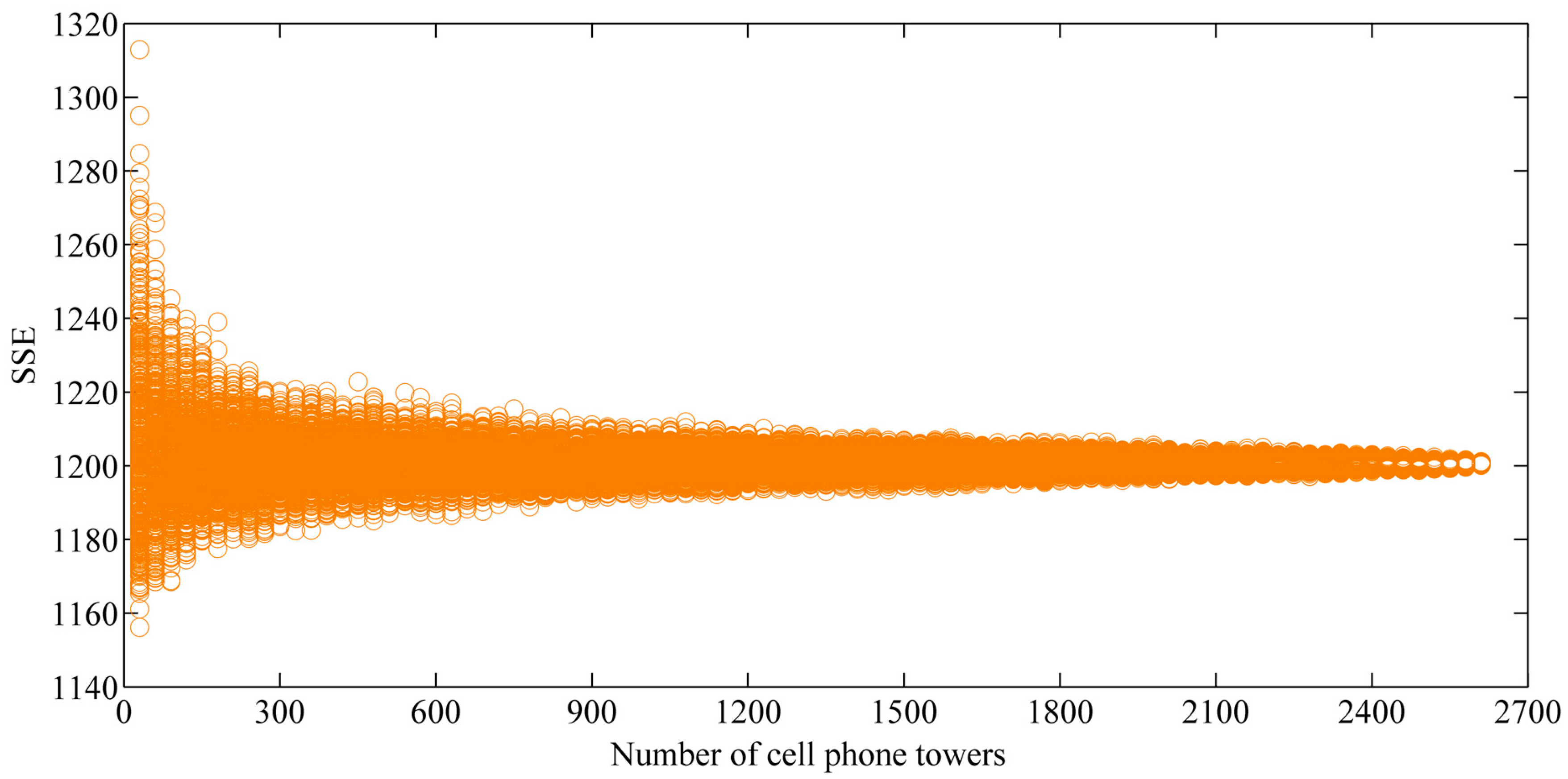
4.1. Distribution of SSE
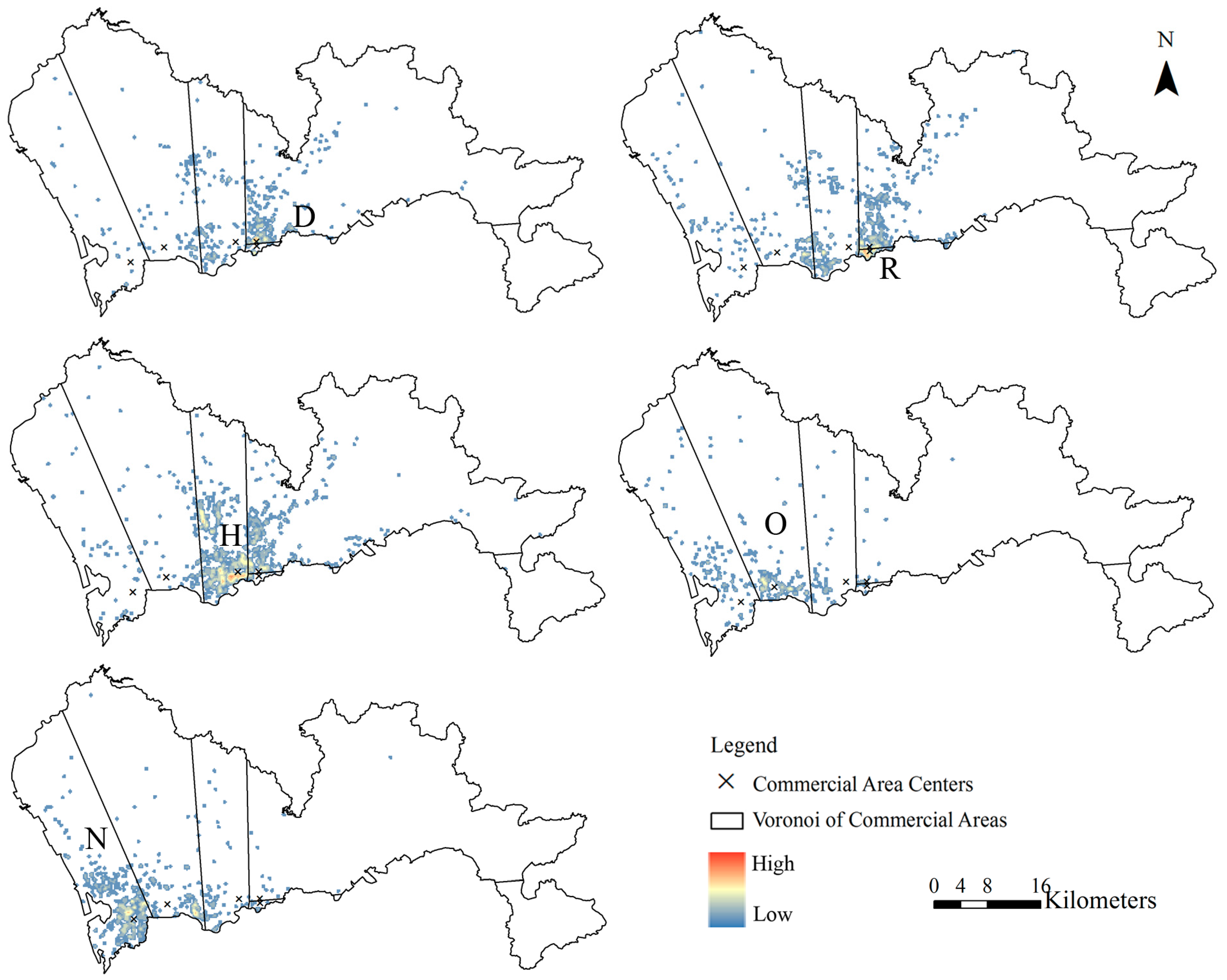
4.2. Finding Out Which Cell Phone Towers Best Fit Each Commercial Area
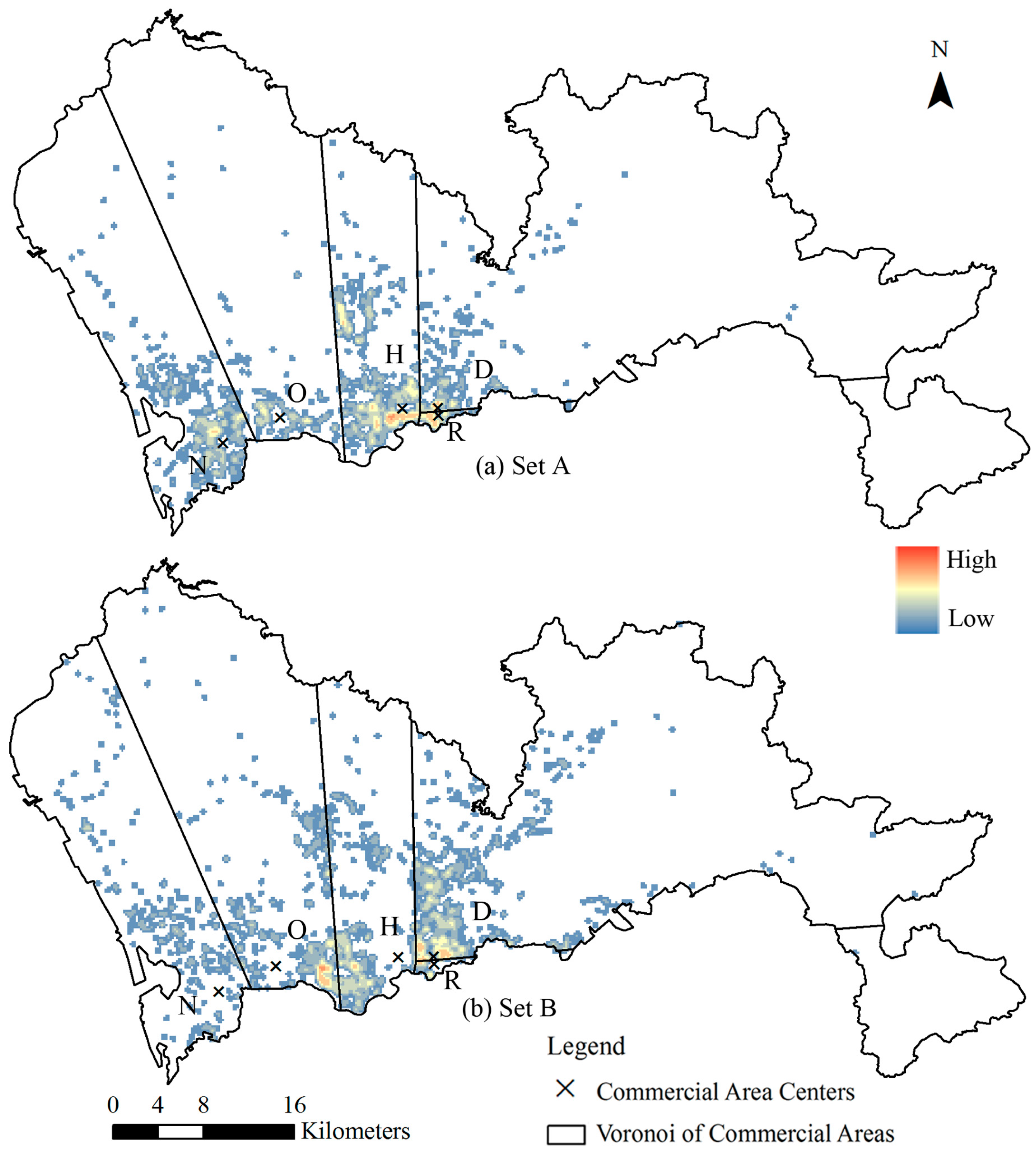
4.3. High-Accuracy Calibration by Using Spatial Adjacency
- (1)
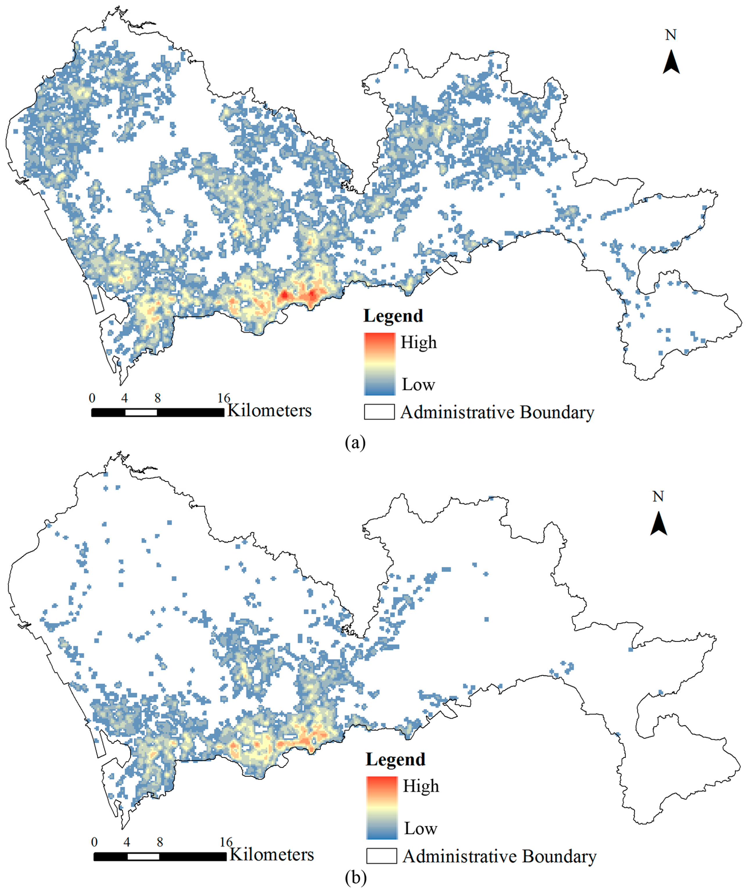
- Set A: The tower’s best fit commercial area is consistent with the tower’s most adjacent commercial area. This subset account for 45.64% of the 2621 cell phone towers, as shown in Figure 7a.
- (2)
- Set B: The tower’s best fit commercial area is not consistent with the tower’s most adjacent commercial area. This subset account for 54.36% of all the 2621 cell phone towers, as shown in Figure 7b.
4.4. High-Accuracy Calibration by Volume of Attracted Tirps
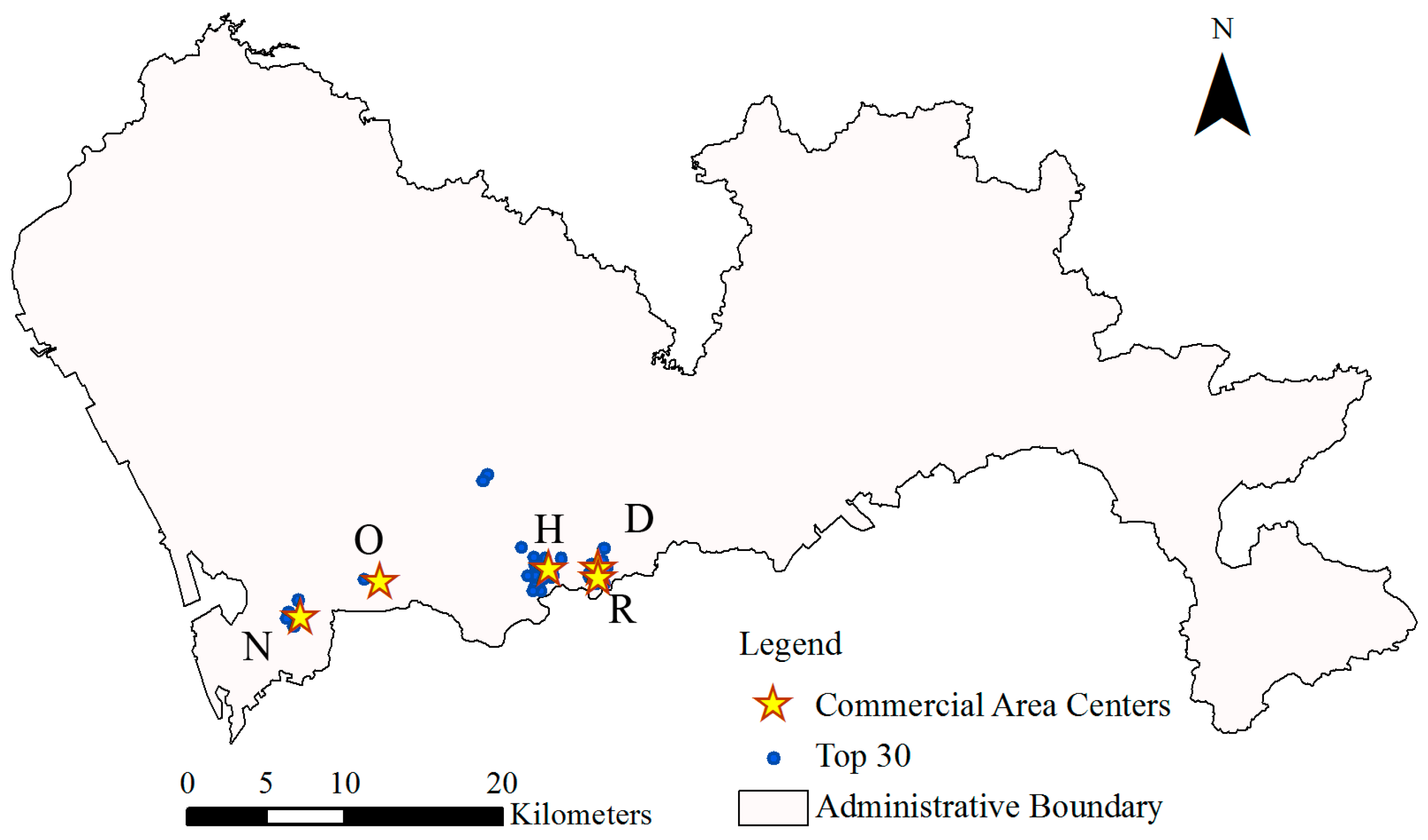
4.4.1. Calibration by Using Top 30 Cell Phone Towers with Highest Trips
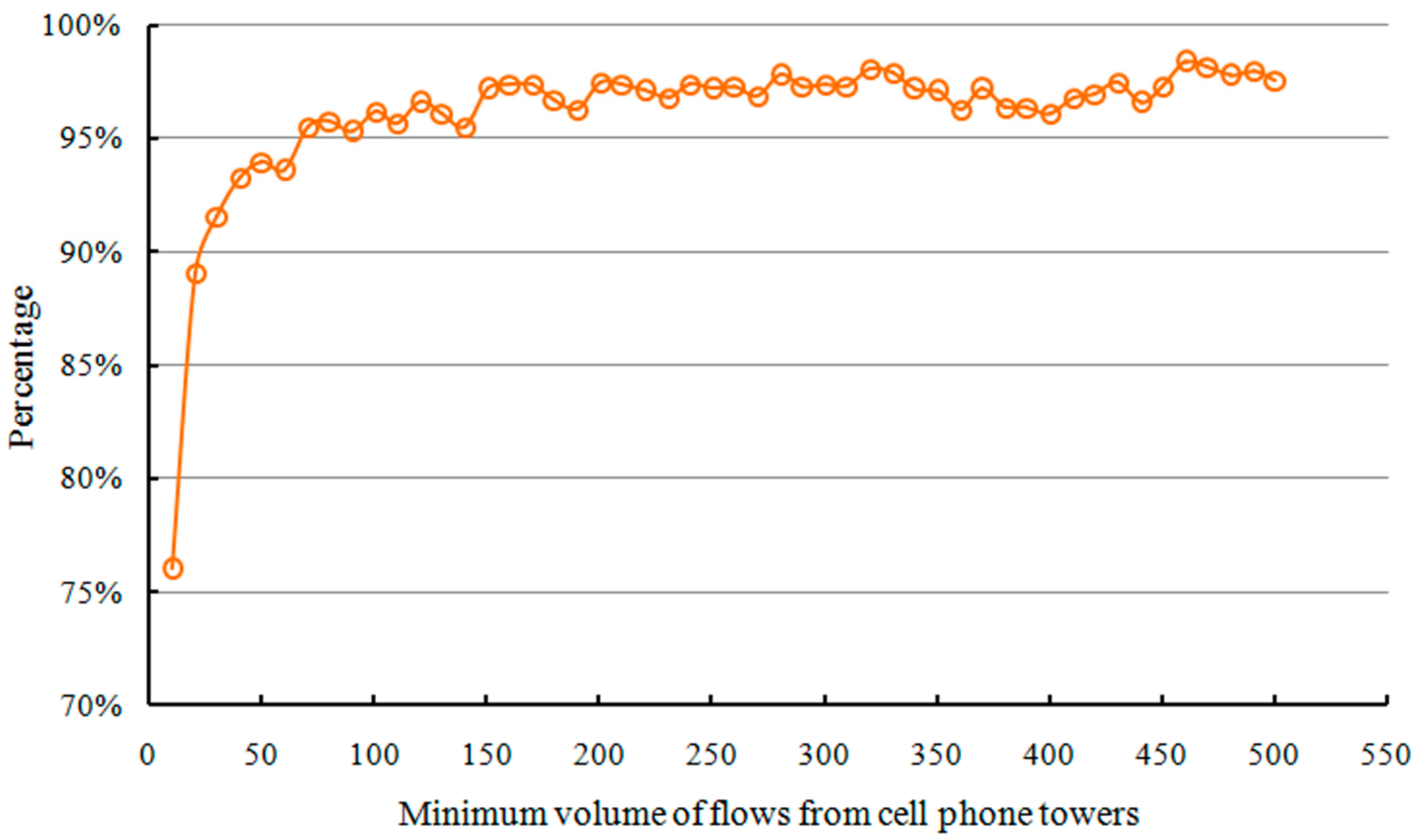
4.4.2. Calibration by Using Selected Towers with Higher Volume of Flows
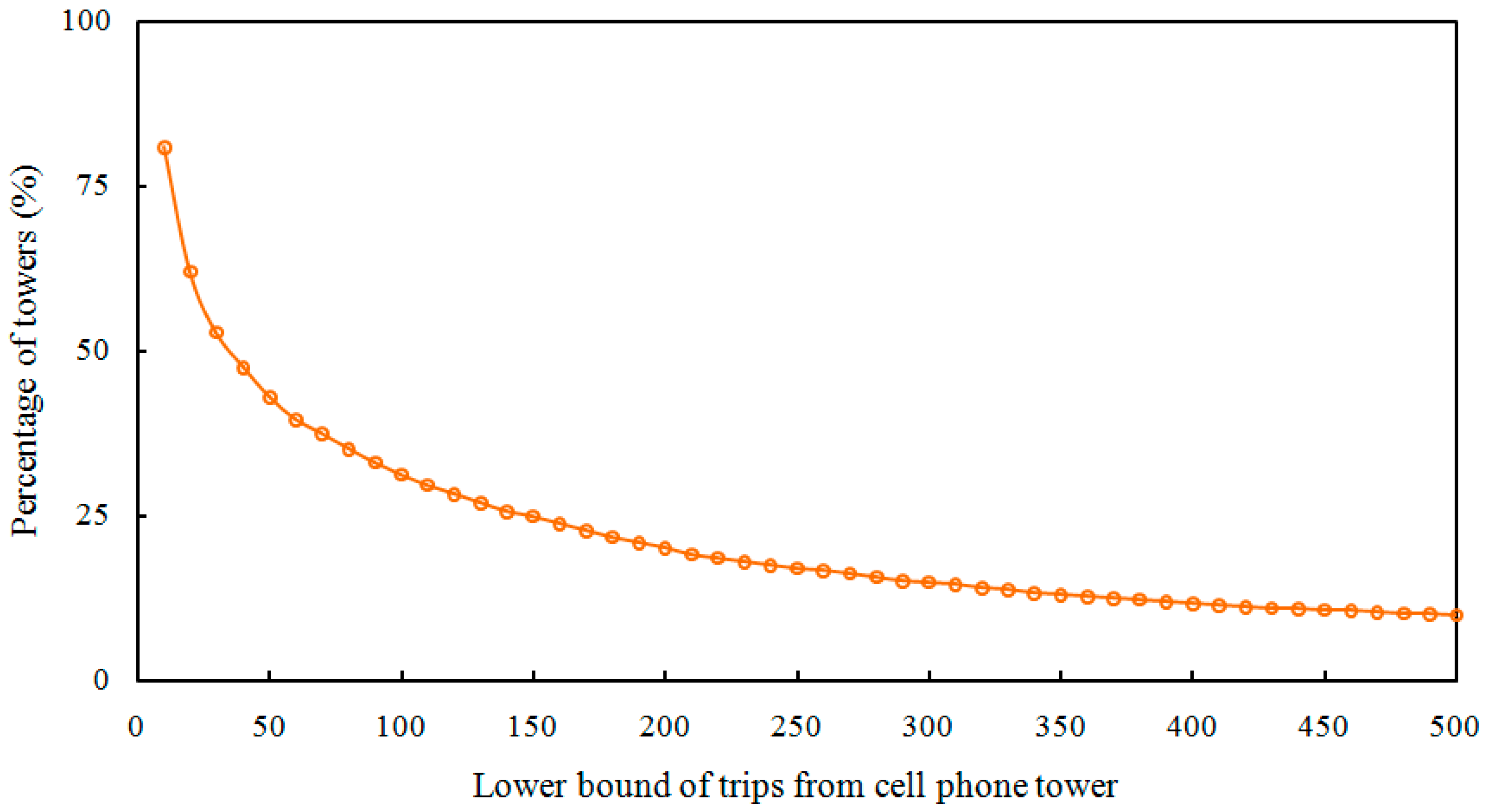
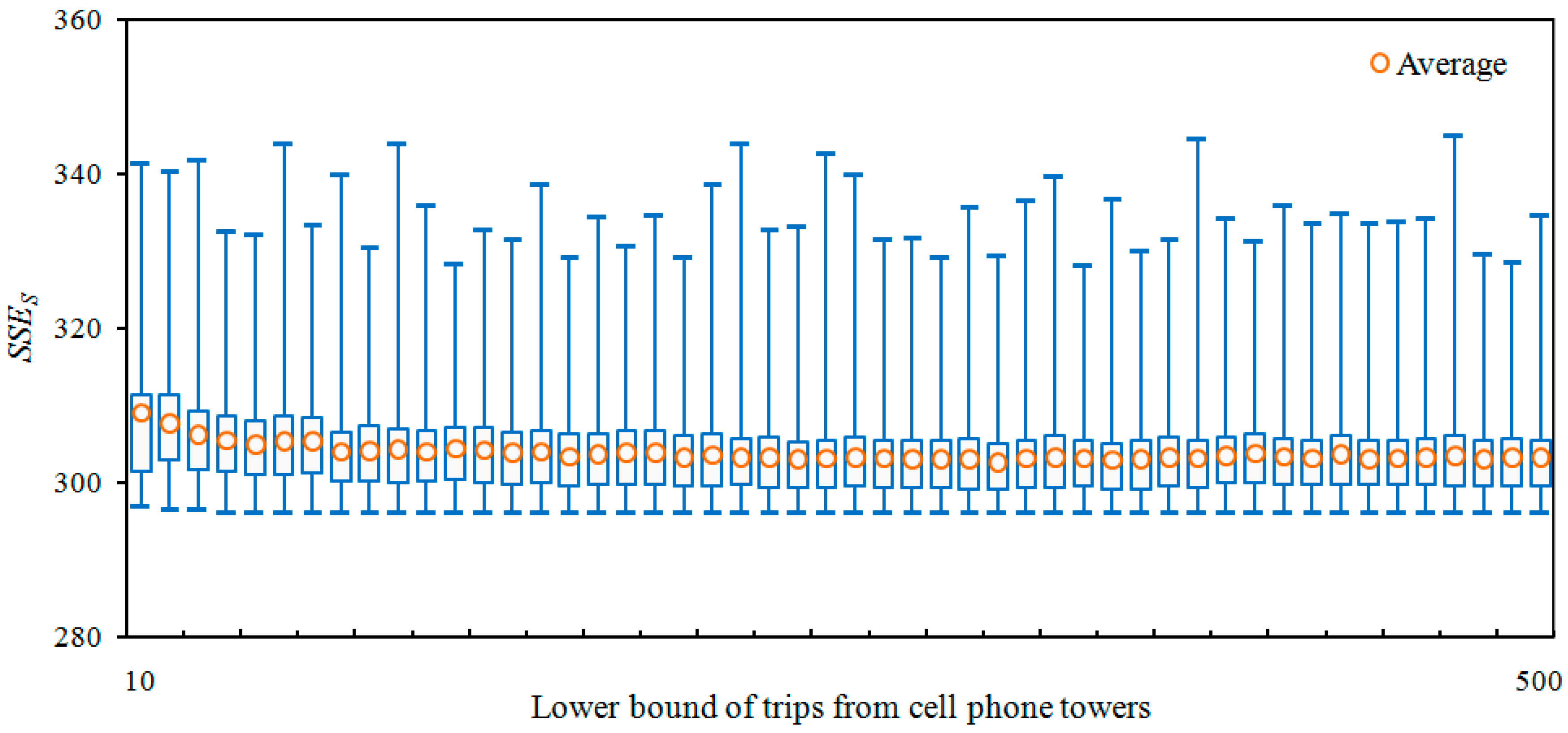
4.4.3. Effects on Towers with “Small” Volume of Trips
5. Conclusions
- (1)
- In this paper, we adopted the Huff model to define business area, and only used size to represent the attractiveness. This simplification created a mismatch between the predicted attracted areas and the observed data. Other factors such as the number of POIs, parking conditions, price level and types of companies, malls in business areas may also influence the attractiveness. In the future, additional research is needed to identify the detailed attractiveness factors and a proper spatial interaction model to better depict the relationships.
- (2)
- Another limitation is that we have not noted the social characteristics of these better performing locations. The combinations of other factors, such as resident distribution, income, land use type and so on, may reveal the social aspects of these better performing locations, which can provide better guidance to surveying or sampling.
- (3)
- In this paper, we investigated the effects of sampling locations on the calibration of spatial interaction model between urban environment and commercial areas. However, our findings may or may not be applicable to other land use types due to the reason that different land use patterns also play a role in the model calibration.
- (4)
- There may be some uncertainties in the extraction of origins/destinations from mobile phone data. It is possible that the “origins” used in this paper were just some passing-by locations, due to the reason that the footprints of mobile phone subscribers were sparsely sampled in space and time [50], so it is hard to limit the “origin” as a “stay” where the subscribers have spent a certain time duration. In the future, dataset like GPS tracking data could be used to reduce the potential uncertainty in extracting the origins or destinations.
Acknowledgments
Author Contributions
Conflicts of Interest
References
- Eppli, M.J.; Shilling, J.D. How critical is a good location to a regional shopping center? J. Real Estate Res. 1996, 12, 459–468. [Google Scholar]
- Lee, M.L.; Pace, R.K. Spatial distribution of retail sales. J. Real Estate Financ. Econ. 2005, 31, 53–69. [Google Scholar] [CrossRef]
- Suárez-Vega, R.; Gutiérrez-Acuña, J.L.; Rodríguez-Díaz, M. Locating a supermarket using a locally calibrated Huff model. Int. J. Geogr. Inf. Sci. 2015, 29, 217–233. [Google Scholar] [CrossRef]
- Lin, T.G.; Xia, J.C.; Robinson, T.P.; Olaru, D.; Smith, B.; Taplin, J.; Cao, B. Enhanced Huff model for estimating Park and Ride (PnR) catchment areas in Perth, WA. J. Transp. Geogr. 2016, 54, 336–348. [Google Scholar] [CrossRef]
- Luo, J. Integrating the Huff model and floating catchment area methods to analyze spatial access to healthcare services. Trans. GIS 2014, 18, 436–448. [Google Scholar] [CrossRef]
- Applebaum, W.; Cohen, S.B. The dynamics of store trading areas and market equilibrium 1. Ann. Assoc. Am. Geogr. 1961, 51, 73–101. [Google Scholar] [CrossRef]
- Ghosh, A.; Rushton, G. Spatial Analysis and Location-Allocation Models; Van Nostrand Reinhold Company: New York, NY, USA, 1987. [Google Scholar]
- Mendes, A.B.; Themido, I.H. Multi-outlet retail site location assessment. Int. Trans. Oper. Res. 2004, 11, 1–18. [Google Scholar] [CrossRef]
- Applebaum, W. Methods for determining store trade areas, market penetration, and potential sales. J. Mark. Res. 1966, 3, 127–141. [Google Scholar] [CrossRef]
- Haines, G.H., Jr.; Simon, L.S.; Alexis, M. Maximum likelihood estimation of central-city food trading areas. J. Mark. Res. 1972, 9, 154–159. [Google Scholar] [CrossRef]
- Wang, Y.; Jiang, W.; Liu, S.; Ye, X.; Wang, T. Evaluating trade areas using social media data with a calibrated huff model. ISPRS Int. J. Geo-Inf. 2016, 5, 112. [Google Scholar] [CrossRef]
- Rodrigue, J.P.; Comtois, C.; Slack, B. The Geography of Transport Systems; Routledge: New York, NY, USA, 2006. [Google Scholar]
- Batty, M. Exploratory calibration of a retail location model using search by golden section. Environ. Plan. A 1971, 3, 411–432. [Google Scholar] [CrossRef]
- Diplock, G.; Openshaw, S. Using simple genetic algorithms to calibrate spatial interaction models. Geogr. Anal. 1996, 28, 262–279. [Google Scholar] [CrossRef]
- Huff, D.L.; McCallum, B.M. Calibrating the Huff Model Using ArcGIS Business Analyst; ESRI White Paper; ESRI: Redlands, CA, USA, 2008. [Google Scholar]
- O’Kelly, M.E. Trade-area models and choice-based samples: Methods. Environ. Plan. A 1999, 31, 613–627. [Google Scholar] [CrossRef]
- Yue, Y.; Lan, T.; Yeh, A.G.O.; Li, Q. Zooming into individuals to understand the collective: A review of trajectory-based travel behaviour studies. Travel Behav. Soc. 2014, 1, 69–78. [Google Scholar] [CrossRef]
- Kirby, H.R.; Leese, M.N. Trip-distribution calculations and sampling error: Some theoretical aspects. Environ. Plann. A 1978, 10, 837–851. [Google Scholar] [CrossRef]
- Watters, J.K.; Biernacki, P. Targeted sampling: Options for the study of hidden populations. Soc. Probl. 1989, 36, 416–430. [Google Scholar] [CrossRef]
- Goodchild, M.F. The quality of big (geo) data. Dialogues Hum. Geogr. 2013, 3, 280–284. [Google Scholar] [CrossRef]
- Lu, S.; Fang, Z.; Shaw, S.L.; Zhang, X.; Yin, L. Quantitative analysis of the effects of spatial scales on intra-urban human mobility. Geom. Inf. Sci. Wuhan Univ. 2016, 41, 1199–1204. [Google Scholar]
- Lu, S.; Fang, Z.; Zhang, X.; Shaw, S.L.; Yin, L.; Zhao, Z.; Yang, X. Understanding the representativeness of mobile phone location data in characterizing human mobility indicators. ISPRS Int. J. Geo-Inf. 2017, 6, 7. [Google Scholar] [CrossRef]
- Haklay, M. How good is volunteered geographical information? A comparative study of OpenStreetMap and ordnance survey datasets. Environ. Plan. B Plan. Des. 2010, 93, 3–11. [Google Scholar] [CrossRef]
- Goodchild, M.F.; Li, L. Assuring the quality of volunteered geographic information. Spat. Stat. 2012, 1, 110–120. [Google Scholar] [CrossRef]
- Zhou, Q.; Li, Z. How many samples are needed? An investigation of binary logistic regression for selective omission in a road network. Cartogr. Geogr. Inf. Sci. 2015. [Google Scholar] [CrossRef]
- Zhao, Z.; Shaw, S.L.; Xu, Y.; Lu, F.; Chen, J.; Yin, L. Understanding the bias of call detail records in human mobility research. Int. J. Geogr. Inf. Sci. 2016, 30, 1738–1762. [Google Scholar] [CrossRef]
- Demirkan, H.; Delen, D. Leveraging the capabilities of service-oriented decision support systems: Putting analytics and big data in cloud. Decis. Support Syst. 2013, 55, 412–421. [Google Scholar] [CrossRef]
- Hashem, I.A.T.; Yaqoob, I.; Anuar, N.B.; Mokhtar, S.; Gani, A.; Khan, S.U. The rise of “big data” on cloud computing: Review and open research issues. Inf. Syst. 2015, 47, 98–115. [Google Scholar] [CrossRef]
- Gonzalez, M.C.; Hidalgo, C.A.; Barabasi, A.L. Understanding individual human mobility patterns. Nature 2008, 453, 779–782. [Google Scholar] [CrossRef] [PubMed]
- Siła-Nowicka, K.; Vandrol, J.; Oshan, T.; Long, J.A.; Demšar, U.; Fotheringham, A.S. Analysis of human mobility patterns from GPS trajectories and contextual information. Int. J. Geogr Inf. Sci. 2016, 30, 881–906. [Google Scholar] [CrossRef]
- Gao, S.; Liu, Y.; Wang, Y.; Ma, X. Discovering spatial interaction communities from mobile phone data. Trans. GIS 2013, 17, 463–481. [Google Scholar] [CrossRef]
- Liu, Y.; Sui, Z.; Kang, C.; Gao, Y. Uncovering patterns of inter-urban trip and spatial interaction from social media check-in data. PLoS ONE 2014, 9, e86026. [Google Scholar] [CrossRef] [PubMed]
- Chi, G.; Thill, J.C.; Tong, D.; Shi, L.; Liu, Y. Uncovering regional characteristics from mobile phone data: A network science approach. Pap. Reg. Sci. 2016, 95, 613–631. [Google Scholar] [CrossRef]
- Ratti, C.; Frenchman, D.; Pulselli, R.M.; Williams, S. Mobile landscapes: Using location data from cell phones for urban analysis. Environ. Plan. B Plan. Des. 2006, 33, 727. [Google Scholar] [CrossRef]
- Xu, Y.; Shaw, S.L.; Zhao, Z.; Yin, L.; Fang, Z.; Li, Q. Understanding aggregate human mobility patterns using passive mobile phone location data: A home-based approach. Transportation 2015, 42, 625–646. [Google Scholar] [CrossRef]
- Balcan, D.; Colizza, V.; Gonçalves, B.; Hu, H.; Ramasco, J.J.; Vespignani, A. Multiscale mobility networks and the spatial spreading of infectious diseases. Proc. Natl. Acad. Sci. USA 2009, 106, 21484–21489. [Google Scholar] [CrossRef] [PubMed]
- Kang, C.; Liu, Y.; Guo, D.; Qin, K. A generalized radiation model for human mobility: Spatial scale, searching direction and trip constraint. PLoS ONE 2015, 10, e0143500. [Google Scholar] [CrossRef] [PubMed]
- Yue, Y.; Wang, H.; Hu, B.; Li, Q.; Li, Y.; Yeh, A.G. Exploratory calibration of a spatial interaction model using taxi GPS trajectories. Comput. Environ. Urban Syst. 2012, 36, 140–153. [Google Scholar] [CrossRef]
- Markham, F.; Doran, B.; Young, M. Estimating gambling venue catchments for impact assessment using a calibrated gravity model. Int. J. Geogr. Inf. Sci. 2014, 28, 326–342. [Google Scholar] [CrossRef]
- Ministry of Industry and Information Technology of the People’s Republic of China. Quarter Book 2016. Available online: http://www.miit.gov.cn/n1146312/n1146904/n1648372/c4802518/content.html (accessed on 3 January 2017).
- Liang, X.; Zhao, J.; Li, D.; Xu, K. Unraveling the origin of exponential law in intra-urban human mobility. Sci. Rep. 2012, 3, 2983. [Google Scholar] [CrossRef] [PubMed]
- Simini, F.; González, M.C.; Maritan, A.; Barabási, A.L. A universal model for mobility and migration patterns. Nature 2011, 484, 96–100. [Google Scholar] [CrossRef] [PubMed] [Green Version]
- Vij, A.; Shankari, K. When is big data big enough? Implications of using GPS-based surveys for travel demand analysis. Trans. Res. Part C Emerg. Technol. 2015, 56, 446–462. [Google Scholar] [CrossRef]
- Batty, M.; Mackie, S. The calibration of gravity, entropy and related models of spatial interaction. Environ. Plann. A 1972, 4, 205–233. [Google Scholar] [CrossRef]
- Wu, C.B.; Sitter, R.R. A model-calibration approach to using complete auxiliary information from survey data. J. Am. Stat. Assoc. 2001, 96, 185–193. [Google Scholar] [CrossRef]
- Roy, J.R.; Thill, J.-C. Spatial interaction modelling. Pap. Reg. Sci. 2004, 83, 339–361. [Google Scholar] [CrossRef]
- Shenzhen Statistical Yearbook 2012. Available online: http://www.sztj.gov.cn/nj2012/indexeh.htm (accessed on 12 September 2016).
- Yang, Y.; Du, Z.; Hua, T. Research on Trade Areas in Other Cities of Pearl River Delta. Available online: http://www.pishu.com.cn/skwx_ps/literature/628924.html (accessed on 19 January 2017).
- Calabrese, F.; Diao, M.; Di Lorenzo, G.; Ferreira, J.; Ratti, C. Understanding individual mobility patterns from urban sensing data: A mobile phone trace example. Trans. Res. Part C Emerg. Technol. 2013, 26, 301–313. [Google Scholar] [CrossRef]
- Becker, R.; Cáceres, R.; Hanson, K.; Isaacman, S.; Ji, M.L.; Martonosi, M.; Rowland, J.; Urbanek, S.; Varshavsky, A.; Volinsky, C. Human mobility characterization from cellular network data. Commun. ACM 2013, 56, 74–82. [Google Scholar] [CrossRef]
- Fotheringham, A.; O’Kelly, M.E. Spatial Interaction Models: Formulations and Applications; Kluwer Academic Pub.: Boston, MA, USA, 1989; Volume 5. [Google Scholar]
- Huff, D.L. A probabilistic analysis of shopping center trade areas. Land Econ. 1963, 39, 81–90. [Google Scholar] [CrossRef]
- Huff, D.L. Defining and estimating a trading area. J. Mark. 1964, 28, 34–38. [Google Scholar] [CrossRef]
- Kim, P.J.; Kim, W.; Chung, W.K.; Youn, M.K. Using new huff model for predicting potential retail market in South Korea. Afr. J. Bus. Manag. 2011, 5, 1543–1550. [Google Scholar]
- Mitchell, A. The ESRI Guide to GIS Analysis: Geographic Patterns & Relationships; ESRI, Inc.: Redlands, CA, USA, 1999; Volume 1. [Google Scholar]
- Strehl, A.; Ghosh, J.; Mooney, R. Impact of similarity measures on web-page clustering. In Proceedings of the Workshop on Artificial Intelligence for Web Search (AAAI 2000), Austin, TX, USA, 30 July–1 August 2000; pp. 58–64.
- Haykin, S.S. (Ed.) Kalman Filtering and Neural Networks New York; Wiley: New York, NY, USA, 2001; pp. 221–269.
- Gold, C.M. The meaning of “neighbour”. In Theories and Methods of Spatio-Temporal Reasoning in Geographic Space; Springer: Heidelberg, Germany, 1992; pp. 220–235. [Google Scholar]


| Commercial Area | D | R | H | N | O |
|---|---|---|---|---|---|
| Area (1000 m2) | 279.10 | 729.20 | 1567.79 | 1155.95 | 1569.92 |
| ID | Date | Time | Longitude | Latitude |
|---|---|---|---|---|
| User1 | 2012/**/** | 07:39:27 | 114. ***** | 22. ***** |
| User1 | 2012/**/** | 08:21:36 | 114. ***** | 22. ***** |
| User1 | 2012/**/** | 08:53:36 | 114. ***** | 22. ***** |
| … | … | … | … | … |
| User2 | 2012/**/** | 03:28:41 | 114. ***** | 22. ***** |
| … | … | … | … | … |
| Cell Phone Towers | Fit D | Fit R | Fit H | Fit O | Fit N | Total |
|---|---|---|---|---|---|---|
| In Polygon D | 23.61% | 34.84% | 37.70% | 2.24% | 1.54% | 100% |
| In Polygon R | 14.89% | 70.22% | 11.70% | 1.06% | 2.13% | 100% |
| In Polygon H | 11.99% | 15.72% | 62.37% | 3.86% | 6.05% | 100% |
| In Polygon O | 12.77% | 19.70% | 12.99% | 28.58% | 25.98% | 100% |
| In Polygon N | 3.38% | 8.82% | 8.26% | 18.20% | 61.35% | 100% |
| Cell Phone Towers | Counts/Percentage | Average | Below 1205 | Above 1205 |
|---|---|---|---|---|
| Set A | 1196 (45.64%) | 1189.3 | 96.2% | 3.8% |
| Set B | 1425 (54.36%) | 1205.4 | 9.2% | 90.8% |
| Average | ≥150 | [100, 150] | [50, 100] | [0, 50] | |
|---|---|---|---|---|---|
| Set A | 370 | 31.9% | 5.9% | 10.9% | 51.1% |
| Set B | 150 | 19.7% | 6.5% | 12.5% | 61.3% |
| Distance (km) | Below Average | Above Average | Counts |
|---|---|---|---|
| [0, 3] | 76.80% | 23.20% | 961 |
| [3, 6] | 52.07% | 47.93% | 742 |
| [6, 9] | 27.92% | 72.08% | 351 |
| [9, 12] | 11.42% | 88.58% | 254 |
| [12, 15] | 5.74% | 94.26% | 122 |
| [15, 18] | 9.72% | 90.28% | 72 |
| [18, 21] | 9.09% | 90.91% | 44 |
| [21, 24] | 3.23% | 96.77% | 31 |
| ≥24 | 18.18% | 81.82% | 44 |
© 2017 by the authors; licensee MDPI, Basel, Switzerland. This article is an open access article distributed under the terms and conditions of the Creative Commons Attribution (CC BY) license (http://creativecommons.org/licenses/by/4.0/).
Share and Cite
Lu, S.; Shaw, S.-L.; Fang, Z.; Zhang, X.; Yin, L. Exploring the Effects of Sampling Locations for Calibrating the Huff Model Using Mobile Phone Location Data. Sustainability 2017, 9, 159. https://doi.org/10.3390/su9010159
Lu S, Shaw S-L, Fang Z, Zhang X, Yin L. Exploring the Effects of Sampling Locations for Calibrating the Huff Model Using Mobile Phone Location Data. Sustainability. 2017; 9(1):159. https://doi.org/10.3390/su9010159
Chicago/Turabian StyleLu, Shiwei, Shih-Lung Shaw, Zhixiang Fang, Xirui Zhang, and Ling Yin. 2017. "Exploring the Effects of Sampling Locations for Calibrating the Huff Model Using Mobile Phone Location Data" Sustainability 9, no. 1: 159. https://doi.org/10.3390/su9010159
APA StyleLu, S., Shaw, S.-L., Fang, Z., Zhang, X., & Yin, L. (2017). Exploring the Effects of Sampling Locations for Calibrating the Huff Model Using Mobile Phone Location Data. Sustainability, 9(1), 159. https://doi.org/10.3390/su9010159