A New Design of High-Performance Large-Scale GIS Computing at a Finer Spatial Granularity: A Case Study of Spatial Join with Spark for Sustainability

Abstract

Sustainability research faces many challenges as respective environmental, urban and regional contexts are experiencing rapid changes at an unprecedented spatial granularity level, which involves growing massive data and the need for spatial relationship detection at a faster pace. Spatial join is a fundamental method for making data more informative with respect to spatial relations. The dramatic growth of data volumes has led to increased focus on high-performance large-scale spatial join. In this paper, we present Spatial Join with Spark (SJS), a proposed high-performance algorithm, that uses a simple, but efficient, uniform spatial grid to partition datasets and joins the partitions with the built-in join transformation of Spark. SJS utilizes the distributed in-memory iterative computation of Spark, then introduces a calculation-evaluating model and in-memory spatial repartition technology, which optimize the initial partition by evaluating the calculation amount of local join algorithms without any disk access. We compare four in-memory spatial join algorithms in SJS for further performance improvement. Based on extensive experiments with real-world data, we conclude that SJS outperforms the Spark and MapReduce implementations of earlier spatial join approaches. This study demonstrates that it is promising to leverage high-performance computing for large-scale spatial join analysis. The availability of large-sized geo-referenced datasets along with the high-performance computing technology can raise great opportunities for sustainability research on whether and how these new trends in data and technology can be utilized to help detect the associated trends and patterns in the human-environment dynamics.

1. Introduction

Sustainability research faces many challenges as respective environmental, urban and regional contexts are experiencing rapid changes at an unprecedented spatial granularity level, which involves growing massive data and the need for spatial relationship detection at a faster pace. The amount and diversity of new data sources have grown dramatically in complex ways at degrees of detail and scope unthinkable until now. As a fundamental method of spatial analysis, spatial join relates an object or event at a certain location to other related data sources in the spatial context. Spatial join links unrelated data using space and, thus, integrates knowledge from scattered sources. It can make data more informative and reveal patterns that may be invisible [1]. For example, researchers quantify the contextual determinants of human behaviors and place-based information by analyzing data from mobile-phone subscribers, social media, floating cars, etc. [2,3,4,5,6]. The size of spatial data has grown dramatically. For instance, in China, the second national land survey has produced about 150 million polygons and 100 million linear roads yearly since 2007. In addition, the first national geography census produced about 2.4 trillion bytes of vector data. These datasets provide a goldmine for sustainability studies across spatial scales. However, existing spatial join tools can only deal with a limited amount of data due to computation constraints. In the face of such massive spatial data, the performance of traditional spatial join algorithms encounters a serious bottleneck. There is a growing consensus that improvements in high-performance computation will pave the new direction for distributed spatial analysis [7]. By deploying a high-performance spatial join computing framework, this study demonstrates that it is promising to leverage cutting-edge computing power for large-scale spatial relationship analysis.

Analyzing the spatial relationship among large-scale datasets in an interdisciplinary, collaborative and timely manner requires an innovative design of algorithms and computing resources. The solutions to these research challenges may facilitate a paradigm shift in spatial analysis methods. The research agenda is being substantially transformed and redefined in light of the data size and computing speed, which can transform the focus of suitability science towards human-environment dynamics in the high-performance computing environment.

Parallelization is an effective method for improving the efficiency of spatial joins [8,9,10,11]. With the emergence of cloud computing, many studies use open source big data computing frameworks, such as Hadoop MapReduce [12] and Apache Spark [13], to improve spatial join efficiency. These Hadoop-like spatial join algorithms including SJMR (Spatial Join with MapReduce) [14], DJ (Distributed Join) in SpatialHadoop [15] and Hadoop-GIS [16]. However, all of them need data preprocessing and cannot perform the entire spatial join in a single MapReduce job; hence, these methods may result in significant disk I/O and additional communication costs. SpatialSpark [17] uses Spark to implement broadcast-based spatial join and partition-based spatial join, then performs an in-depth comparison with SpatialHadoop and Hadoop-GIS [18]. Inheriting the advantages, such as low disk I/O and in-memory computing, of Spark, SpatialSpark improves the join efficiency significantly.

For distributed spatial join in a Hadoop-like framework, spatial data partition is a key point that affects the performance of spatial join. All current algorithms use the following method to do spatial partition: (1) sample the datasets to reduce the data volume; (2) create a spatial index on one or both dataset; (3) use the spatial index to partition the datasets or map the indexes, then do global join directly. However, all of the methods partition the datasets based on the spatial index, which considers the data size or number of data only, which may cause the processing skew of each partition. SpatialSpark partitions both input datasets with the spatial index of one dataset, thus resulting in an imbalance because of the data skew mismatch of the two datasets. Furthermore, both sampling and spatial indexing require extra computing cost, which is expensive, especially for the MapReduce framework. Faced with massive vector data, the performances of current Hadoop-like spatial join algorithms run into a bottleneck.

Based on the analysis of existing Hadoop-like high-performance spatial join algorithms, we found that the key factors for improving the performance of spatial join are: (1) simplification of the spatial partitioning algorithm to reduce the preprocessing time; (2) optimization of the partition results for both CPU and memory requirements; and (3) improvement of the performance of the local join algorithm. In this study, we propose a new spatial join method with Spark: Spatial Join with Spark (SJS). SJS uses a proven, extremely efficient fixed uniform grid to partition the datasets. Global join is achieved through built-in join transformation. Utilizing the iterative computation of Spark, we propose a calculation evaluating model and in-memory spatial repartition technology, which refine the initial partition results of both datasets to limit the processing time of each partition by estimating the time complexity of the local spatial join algorithm. In the last local join stage, we implement and compare the performances of plane-sweep join, R-tree, quadtree and R*-tree index nested-loop join. The experiments show that the R*-tree index nested-loop join is the best method with regard to high space utilization and query efficiency. From extensive experiments on real data, it is observed that SJS performs better than the earlier Hadoop-like spatial join approaches.

This research focuses on solving the computation challenge emerging from the large data size, which will serve as the solid foundation for further spatial analysis with other covariates and contextual information.

The main contributions of this study are as follows:

(1)

We propose SJS, a universally-distributed spatial join method with Spark. Experiment results show that SJS exhibits better performance than the earlier Hadoop-like spatial join approaches.

(2)

We utilize the in-memory iterative computing of Spark and present a non-disk I/O spatial repartition technology to optimize the initial partition based on the calculation-evaluating model.

(3)

We make performance comparisons among four common in-memory spatial join algorithms in Spark and conclude that the R*-tree index nested-loop join exhibits better performance than other algorithms in a real big data environment.

2. Background and Related Work

2.1. Spark Parallel Computing Framework

Spark is a fast and general engine for large-scale data processing. When compared with MapReduce, the most significant characteristics of Spark are the support for iterative computation on the same data and distributed in-memory computing. Spark uses Resilient Distributed Datasets (RDD) [19] to “transform”-persistent datasets on a disk to distributed main memory and provides a series of “transformations” and “actions” to simplify parallel programming. Spark inherits the advantages of MapReduce, such as high scalability, fault tolerance and load balancing. Further, Spark overcomes challenges, such as iterative computing, join operation and significant disk I/O and addresses many other issues. Currently, Spark is widely used in high-performance computing with big data. In addition, any MapReduce project can easily “translate” to Spark to achieve high performance.

2.2. Spatial Join Query

The spatial join method includes two-way and multi-way spatial join. It is a basic GIS tool to conduct impact assessments of change and development. This study focuses on two-way spatial join. For spatial datasets R and S, the two-way spatial join is defined as follows:

$$\text{SpatialJoin}\left(R,S\right) = \left\{\left(r,s\right)|r \in R,s \in S\right\},\text{where} SP\left(r,s\right) = \text{true}$$

(1)

where SP is a spatial predicate for the relationship between two spatial objects. A spatial predicate can be a topological relationship or spatial analysis function, such as the K Nearest Neighbor (KNN) query and buffer analysis. A spatial join is typically performed in two stages [20]: filter stage and refinement stage. In the filter stage, each $r \in R \mathrm{and} s \in S$ is expressed as an approximation, such as a Minimum Boundary Rectangle (MBR). Then, all of the pairs in R and S whose MBRs overlap are determined. In the refinement stage, each spatial approximate pair is restored to the full object pair, and finally, the object pairs that satisfy the given spatial predicate are provided as output.

Without any optimization, the time complexity of the basic nested loop spatial join is $O(\Vert R\Vert \times \Vert S\Vert )$, where $\Vert R\Vert$ and $\Vert S\Vert$ represent the sizes of the two join datasets, R and S, respectively. Certain improved methods that can be classified as internal and external memory spatial join have been proposed, such as plane-sweep [21], iterative spatial join [22], Partition Based Spatial-Merge join (PBSM) [11], TOUCH [23] and the index nested-loop join using R-tree [24], R*-tree [25] or quadtree. In spatial index synchronous approaches, spatial join is performed by indexing both datasets with a single [26] or double [8] R-tree variant. However, all of these approaches focus on the basic improvement of spatial join algorithms in a single-node case, which is difficult for managing massive spatial datasets.

Parallelization is an effective method for improving the performance of spatial join. The concept of parallel spatial join originated in the 1990s. The early parallel spatial join methods focused on fine-grained parallel computing, the creation of a spatial index in parallel and synchronous traversal of the index to perform a spatial join [8]. As data size increases, these parallel algorithms are no longer suitable. Patel and DeWitt evaluated many parallel partition-based spatial join algorithms in parallel databases and recommend the use of clone and shadow join [27]. Zhou et al. proposed the first parallel spatial join method based on grid partition [10]. Hoel and Samet [28] presented efficient data-parallel spatial join algorithms for PMR quadtrees and R-trees; spatial objects (line segments in the paper) are organized using hierarchical spatial data structures and joined through the map intersection. The Scan-And-Monotonic mapping (SAM) model is used for parallel computing. However, all of the spatial decomposing strategies in these approaches are based only on the number or size of objects in one or both datasets. None considers the computing cost of spatial join algorithms in each partition.

Many other works focus on parallel spatial join in distributed spatial databases. Niharika [29] is a parallel spatial data analysis infrastructure that exploits all available cores in a heterogeneous cluster. Spatial declustering in Niharika aims to assign neighboring tiles to the same node and reduce the data skew. However, the partition strategy in Niharika considers memory only; in other words, the recursive tiling is only based on the numbers of objects, which may cause uneven spatial join processing in each partition, especially when the number of objects of the two datasets are similar in the same partition. Skew-resistant Parallel IN-memOry spatial Join Architecture (SPINOJA) [30] focuses on the performance of the refinement stage by considering that the efficiency bottleneck is the processing skew caused by the uneven work metrics, including object size and point density. However, in this approach, objects ore decomposed by clipping against the tile boundaries in order to reduce processing skew on large objects, which could require additional storage space or calculation costs and increase the number of objects. In addition, SPINOJA focuses mainly on the running time of the refinement stage, but ignores the time complexity of the entire spatial join algorithms.

2.3. Hadoop-Like Spatial Join Approaches

MapReduce is a new and popular platform to parallelize spatial join. The first spatial join algorithm with MapReduce, SJMR [14], uses the map function to divide the uniform space into grid tiles ordered by Z-value and then maps the tiles to partitions using a round-robin approach to balance the processing. Then, each partition corresponds to a reducer, and the reduce function executes the local join. However, this study does not improve the performance by refining the grid-partition or using the spatial index.

SpatialHadoop is a MapReduce extension to Apache Hadoop designed specifically for spatial data. Eldawy and Mokbel [15] presented a MapReduce-based spatial join method built in SpatialHadoop. The method consists of three phases: (1) in the preprocessing stage, spatial indexes are created and used to partition the datasets; (2) in the global join stage, a new MapReduce job is created to join the partition and perform repartitioning, if necessary; and (3) in the local join stage, the filter and refinement step of each partition pair is performed using the pre-created spatial indexes. Thus, the algorithm includes at least two MapReduce jobs, and all intermediate results are serialized to the Hadoop Distributed File System (HDFS), which results in significant disk I/O. Further, although a partition with R+-tree can achieve better space utilization, it is considerably more time consuming, whereas a partition with the grid index consumes less time, but yields a result that is affected by data skew. A repartition step was designed to refine the partitions and only consider the memory and a single dataset; this step increases the burden of disk access for additional MapReduce jobs.

An improved spatial partitioning method, Sample-Analyze-Tear-Optimize (SATO) [31] in Hadoop-GIS [16], has been proposed. Using SATO, Hadoop-GIS reduces data skew in the preprocessing stage. In the local join stage, Hadoop-GIS builds an R*-tree on both datasets to perform a synchronous traversal spatial join. However, the spatial join in Hadoop-GIS, which is based on MapReduce, also has the same limitations as SpatialHadoop and SJMR.

The increasing demand for real-time computing has resulted in the emergence of many distributed in-memory computing frameworks, such as Apache Spark, which offer the potential of further improving the efficiency of spatial join. Some Spark-based spatial processing engines have been developed in the last several years, such as SpatialSpark, GeoSpark, SparkGIS and Simba.

SpatialSpark implements broadcast-based [17] and partition-based [18] spatial join with Spark. Broadcast-based spatial join resembles a “global” index nested-loop join. A spatial index is created on one dataset and broadcast to all nodes. Then, the other dataset is read into the main memory in the form of RDD and then traversed to perform an index nested-loop join with map transformation. However, this approach is suitable only for the point-in-polygon spatial join. The growth of the polygon dataset can cause the index building or broadcasting and in-memory storage to become a bottleneck, specifically in the case of insufficient main memory.

Partition-based spatial join uses the SATO partition method provided by Hadoop-GIS, but the partition method is applied on only one dataset. By querying the same index that is created after SATO, the Spark built-in join transformation is used to perform global join, which is more efficient. SpatialSpark avoids repartitioning and implements the local join using the index nested-loop in-memory join method. Finally, the built-in distinct transformation is used to remove duplicates after refinement; unfortunately, repetitive calculations already occur. In the case of SpatialSpark, the researchers believe that the partition result of SATO on one dataset is also applicable to the other dataset, and hence, they did not implement any refinement in the following stage. However, in most cases, the two datasets might not have the same data-skew; searching for the same index in one dataset could cause a serious skew in the other set. Although the in-memory parallel framework of Spark can handle skew by default, the extremely large partitions could lead to CPU and memory overload. In addition, duplicates are not avoided in a timely manner before the refinement phase of the local join phase. Furthermore, the researchers did not conduct a performance analysis of the Spark submit parameters or a comparison of the various in-memory spatial join methods.

GeoSpark [32] extends Spark with a Spatial Resilient Distributed Datasets (SRDD) layer and a spatial query processing layer. The approach of spatial join in GeoSpark does not involve any algorithm refinement. Spark-GIS [33], the Spark version of Hadoop-GIS, implements spatial join based on the Hadoop-GIS Real-time Spatial Query Engine (RESQUE). In addition, Spark-GIS improves the computational efficiency mainly through the Spark framework instead of the algorithm refinement. Simba [34] extends the Spark SQL engine to support rich spatial queries and analytics. Their studies mainly focus on providing a user-friendly programming interface and building a spatial query planner or optimizer. Spatial join in Simba concentrates on distance join instead of topological join as SpatialSpark and our approach do. As SpatialSpark first proposed a comprehensive Spark-based spatial join and others made few improvements, our approach mainly compares with SpatialSpark.

3. Methods

This section describes a novel spatial join method, SJS, that combines the key concept of clone-join with index nested-loop join and is implemented with Spark. The SJS phases are summarized as follows:

Phase 1. 

Partition phase: perform parallel calculation of the partition IDs of the uniform grid for each spatial object.

Phase 2. 

Partition join phase: group the objects with the same partition ID in each dataset, and join the datasets with the same partition ID.

Phase 3. 

Repartition phase: evaluate the calculation costs of each partition, and repartition those partitions whose costs result in overrun.

Phase 4. 

In-memory join phase: perform the R*-tree index nested-loop join on each repartition.

Different from other Hadoop-like spatial join algorithms, the SJS partition phase does not perform additional tasks, such as data sampling and spatial index building on one or both datasets, and does not execute any partition packaging or sorting tasks, such as round-robin tile-to-partition mapping [35] and Z-curve or Hilbert tile coding sort [36]. The reason for this behavior is discussed in Section 3.1. The partition join phase (similar to the global join phase) of SJS differs from MapReduce-based join methods because it uses a built-in join transform in Spark instead of separating the “IndexText” of the reduced input value. Next, the initial partition results are repartitioned by evaluating the time complexity of the in-memory join in each partition to decrease the process skew. All SJS repartition tasks are performed in memory with the RDD transformation, which improves the performance by eliminating the disk I/O. The in-memory join phase (similar to the local join phase) of SJS differs from the plane-sweep in SJMR or SpatialHadoop and the synchronous traversal of both R*-trees on each dataset in Hadoop-GIS. In this phase, SJS uses a single R*-tree index built on one dataset and traverses the other dataset in order to perform the index nested-loop join. Duplicates are avoided using the reference point method before calculating.

3.1. Uniform Spatial Grid Partition

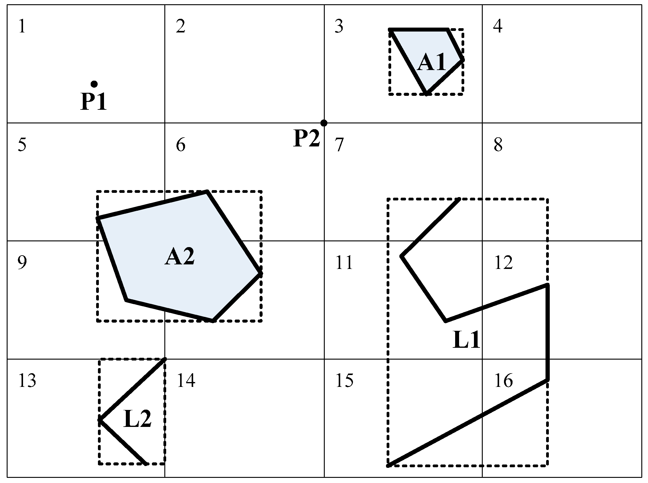
The goal of spatial partitioning is to reduce the data volume such that it fits in the memory and to perform coarse-grained parallel computing (bulk computing). As shown in Figure 1, Grid Tiles 1–16 represent the uniform grids. The spatial objects are partitioned into the tile overlap with their MBRs.

Grid count is the key factor in the algorithm. If the number of grids is low, each partition fitting in the memory or the CPU computing requirements cannot be guaranteed. If the number of grids is high, the large number of duplicates could increase the calculation. Therefore, we determine the number of partitions in a manner similar to the method described in [11]. Furthermore, we propose a dynamic spatial repartition technology to refine the partition result.

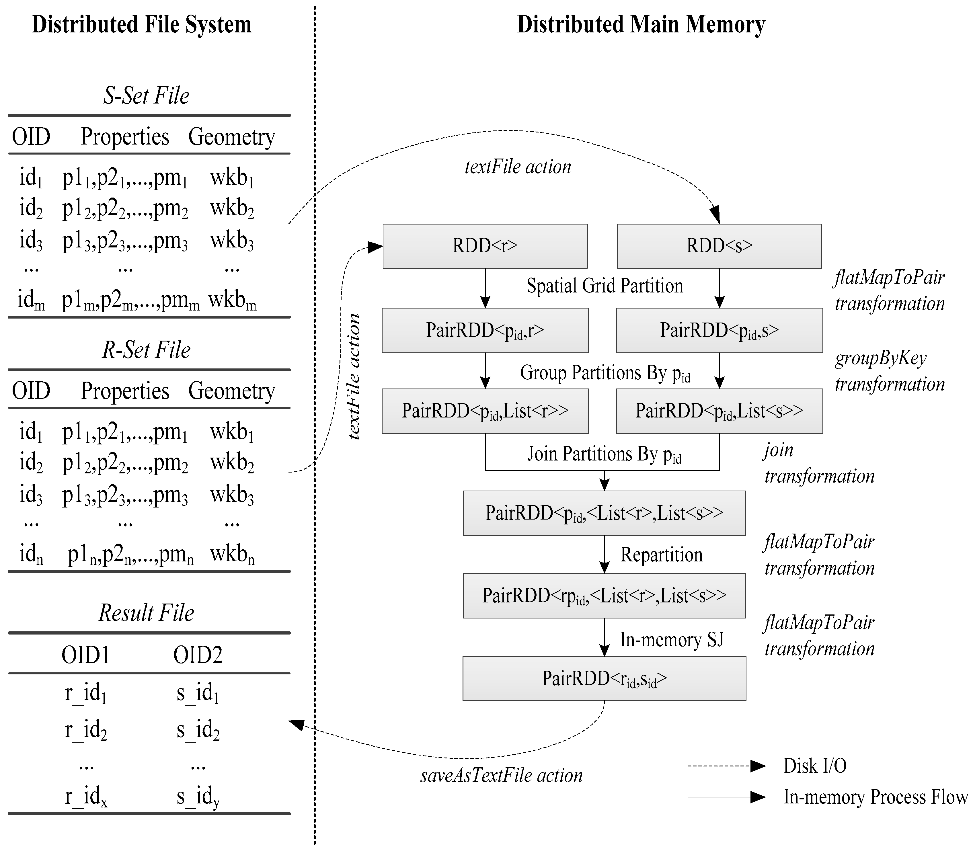
For datasets R and S stored in the distributed file system, we use the “textFile” action in Spark to read the files to RDDs cached in the distributed main memory. Then, the “flatMapToPair” transformation, indicated in Algorithm 1, is used to perform the spatial partitioning. Each flatMap calculates the grid tiles that overlap with their MBR. Then, the spatial partitioning phase returns the pairs of partition ID and geometry of each spatial object.

Algorithm 1 Spatial Partitioning

PairRDD<Partition ID, Geometry>$\leftarrow$RDD<Geometry>.flatMapToPair(SpatialPartition)

Input: line: each line of spatial dataset file

Output: R: partitioned objects

Function SpatialPartition(line)

1 $R=\varnothing ;$

2 $o=read the geometry of the spatial object from line;$

3 $T=o tain overlap grid tiles of o.MBR;$

4 $\mathit{f}\mathit{o}\mathit{r}\mathit{e}\mathit{a}\mathit{c}\mathit{h} t \in T \mathit{d}\mathit{o}$

5 $R\leftarrow R{{\displaystyle \cup }}^{\text{}}\left(t.getID,o\right);$

6 $\mathit{e}\mathit{m}\mathit{i}\mathit{t}\left(R\right);$

3.2. In-Memory Spatial Partition Join

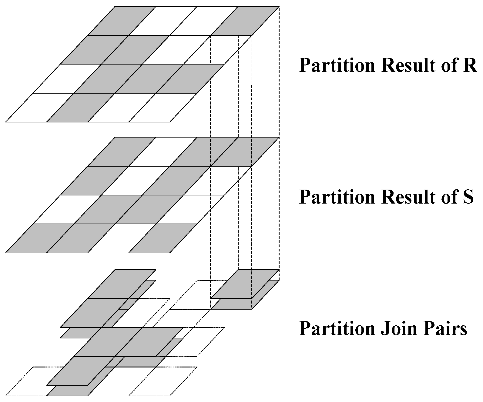
This phase consists of the following two steps. Step 1: group the spatial objects of both the datasets with the same partition ID using the “groupByKey” transformation in Spark. Step 2: use the “join” transformation to join both datasets with the same partition ID. As shown in Figure 2, the first and second layers represent the R and S dataset partition groups, respectively. A gray tile implies that it contains at least one spatial object, whereas a white tile implies that there are no spatial objects inside it. The partitions are joined, and the result is shown in the third layer. The operation executes only on the partitions whose corresponding R and S partitions are gray. Partitions with only one or no gray partitions are removed from the main memory.

The spatial join operation of the entire R and S datasets is reduced to the join operation on the partition pairs; this is the first filter of the entire spatial join. By utilizing this feature, SJS reduces disk I/O costs further in the partition phase when compared with other spatial join techniques with MapReduce [15,16], where the objects in the dotted partition as shown in Figure 2 are moved to the disk in order to execute the reduce function.

3.3. Calculation Evaluating-Based Spatial Repartition Technology

3.3.1. Spatial Repartition Strategy in Spark

From the previous two phases, we know that the proposed spatial partition refers to uniform grid tiles. As mentioned in Section 3.1, the goal of spatial partitioning is to reduce the amount of data in order to accommodate data in the memory of nodes and to increase computational parallelism. However, based on the grids specified for the partitioning of spatial data and considering the data skew and data replication, partitions that contain an excessive number of spatial objects would directly affect the performance of the overall spatial join.

The traditional method is to reset the grid size and repartition the dataset to meet the requirements. However, this approach discards the initial partition computation, and the partition results after adjustment might still not meet the requirements. Another method is to optimize the partition strategy, by iteratively decomposing the tiles when the number of objects in the partition exceeds the threshold. This strategy contributes to limiting the size of data in each partition, but only works on one dataset, respectively, and requires an additional structure to map the partitions of two datasets. In particular, this strategy considers memory only; the uniform total number in each partition cannot guarantee uniform processing time, and thus, the CPU cost in each partition must be taken into consideration. In the most recent spatial join algorithms with MapReduce, the spatial partitioning occurs during the entire map stage or MapReduce job, and the partition results must be written to HDFS for subsequent calculations. When the partition fails, the entire process must be executed again, thus resulting in considerable unnecessary disk I/O.

The Directed Acyclic Graph (DAG) scheduler of Spark dispatches the calculation of each partition to those nodes whose current number of running tasks has not reached the maximum number. Thus, when a node completes a task, the next task is allocated to the node and executed immediately. The total number of tasks that run on each node is considerably fewer than the number of partitions; hence, the bottleneck of spatial join in Spark is the extremely large partition caused by data skew and not the lack of balance in the intensity of the partition. Therefore, we use grid tiles as partitions directly and the tile ID as the partition ID.

Based on this analysis, if data skew or a large number of data replications occur, the bottleneck of spatial join is the overhead from the calculation of partitions. When the original grid is not sufficiently appropriate, the large partition could lead to CPU overload. Hence, the repartition strategy for refinement in Spark must take the calculation amount of large partitions into consideration. We propose an improved in-memory spatial repartition method based on the calculation amount of local join algorithms in order to refine the partition results.

3.3.2. Calculation Evaluating Model

For partition P, we define the calculation evaluating model as follows:

$$CalculationAmount\left(P\right) = f \left(n,p,O\right)$$

(2)

where O denotes the time complexity of the algorithm; n denotes the number of spatial objects in P; p denotes the total number of vertices of every object in P, which also refers to the complexity of objects. For different algorithms, the valid parameters and parameter values are different. For instance:

(1)

For the area calculating algorithm, the time complexity is only related to parameter p:

$$CalculationAmount\left(P\right) = f \left(null,p,O\left(p\right)\right) = p$$

(3)

(2)

For the nested-loop spatial join algorithm, the time complexity is mainly related to parameter n:

$$CalculationAmount\left(P\right) = f \left(\left(n_r,n_s\right),null,O\left(n_r·n_s\right)\right) = n_r\times n_s$$

(4)

Here, since after partition join, each P contains spatial objects belong to R and S, thus n is expressed as tuple $\left(n_r,n_s\right)$. $n_r$ denotes the number of spatial objects that belong to R in P, the same with $n_s$.

This study uses the calculation evaluating model to compute the calculation amount of each partition, then judges the partition for whether it needs repartition or not. Repartition is a course of iteration, so a Threshold Value (TV) is imported to terminate recursion. For dataset R, we define the Equation of TV as follows:

$$TV=f\left(N,S,M\right)= k\times \frac{N\times M}{S}$$

(5)

where N denotes the number of objects in R; S denotes the data size of R; M denotes the total allocated memory size of all nodes; k denotes the ratio factor, which is determined by the algorithm. For the R*-tree index nested-loop spatial join algorithm, we set k = 0.01 as the reference value.

3.3.3. Spatial Repartition Phase in SJS

In SJS, the partitions of two datasets are joined directly without any other correspondence or mapping, such that the repartition strategy can consider both datasets. Because the objects of two datasets are cached as forms of RDD in memory, disk I/O skew no longer exists. Thus, the repartition phase in SJS focuses mainly on the processing skew of each partition. In order to evaluate the calculation amount of the in-memory spatial join algorithm and estimate the CPU consumption of each partition, we choose the typical nested-loop spatial join to represent others. In the calculation evaluating model, we use Equation (4) to calculate the valuation. By setting a threshold value using Equation (5), the calculation amount of each partition is limited.

Spark supports iterative calculation with the same data; any intermediate results from the calculations are cached in memory in the form of RDD. We use the “flatMapToPair” transformation to transform the initially-partitioned RDD to the repartitioned RDD. As shown in Algorithm 2, first, the sizes of R and S within the current partition are calculated; if their product (the valuation) is greater than a preset threshold value, the current partition is divided into four equivalent sub-partitions, and the divide and replicate strategy is the same as that in the previous phase. If the product is less than the threshold value, the original partition is returned. Algorithm 2 executes recursively (Line 12) on each initial partition distributed among the nodes; the iterative processes need not communicate with each other. Thus, the in-memory spatial repartition technology completely utilizes the advantage of the in-memory computing architecture of Spark, and the disk I/O is reduced to a minimum. The repartition result is sufficient for the various in-memory join algorithms to execute the next phase.

Algorithm 2 Dynamic In-Memory Spatial Repartition

PairRDD<pid, Tuple<RP, SP>>$\leftarrow$PairRDD<pid, Tuple<RP, SP>>.flatMapToPair (Repartition)

Input: RP, SP: two partial datasets in current partition;

pid: ID of current partition

Output: RP: the repartition result of the current partition

Data: TV: preset threshold value

Function Repartition (pid, RP, SP)

1 $RP=\varnothing ;$

2 $n=size of R_P;$

3 $m=size of S_P;$

4 $\mathit{i}\mathit{f} n \times m \ge TV \mathit{t}\mathit{h}\mathit{e}\mathit{n}$

5 $R_{RP},S_{RP}=\varnothing ;$

6 $R_{RP}=repartition R_P to four equal sub-parts;$

7 $S_{RP}=repartition S_P to four equal sub-parts;$

8 $\mathit{f}\mathit{o}\mathit{r}\mathit{e}\mathit{a}\mathit{c}\mathit{h} r_{rp} \in R_{RP} and s_{rp} \in S_{RP} \mathit{d}\mathit{o}$

9 $r{p}_{id}=sub-part id;$

10 $\mathit{i}\mathit{f} r_{rp}\ne \varnothing and s_{rp} \ne \varnothing \mathit{t}\mathit{h}\mathit{e}\mathit{n}$

11 $RP\leftarrow RP{{\displaystyle \cup }}^{}\left(r{p}_{id,}{r}_{rp,}{s}_{rp}\right);$

12 $RepartitionFun\left(r{p}_{id,}{r}_{rp,}{s}_{rp}\right);$

13 $\mathit{e}\mathit{l}\mathit{s}\mathit{e}$

14 $RP=\left(p_{id},R_P,S_P\right);$

15 $\mathit{e}\mathit{m}\mathit{i}\mathit{t}\left(RP\right);$

3.4. In-Memory Spatial Join

After the partition adjustment, theoretically, we can use any type of in-memory method to complete spatial join. All spatial entities have been cached as RDD, and hence, we can process the filter and refinement step of the spatial join synchronously. Furthermore, the traditional random access of data entities in the refinement stage, which could lead to high disk I/O costs, will be omitted. In this study, we implement four methods, i.e., the classic plane-sweep, in addition to the R-tree, R*-tree and quadtree index nested-loop join. Finally, we choose the R*-tree index for SJS because of its high space utilization and the retrieval speed. Several experiments show that the R*-tree index nested-loop join has better performance in most cases. The R*-tree nested-loop join is described as follows (see Algorithm 3):

Algorithm 3 R*-Tree Nested-Loop Join

PairRDD<rid, sid>$\leftarrow$PairRDD<pid, Tuple<RP, SP>>.flatMapToPair(LocalJoin)

Input: pid: ID of current partition

RP, SP: two spatial datasets in the current partition;

Output: P: the spatial join result pairs of the current partition

Function LocalJoin(pid, RP, SP)

1 $P=\varnothing ;$

2 $I=build R*-tree index of R_P;$

3 $\mathit{f}\mathit{o}\mathit{r}\mathit{e}\mathit{a}\mathit{c}\mathit{h} s \in S_P \mathit{d}\mathit{o}$

4 $T=search I by s.MBR for overlap items;$

5 $\mathit{f}\mathit{o}\mathit{r}\mathit{e}\mathit{a}\mathit{c}\mathit{h} t \in T \mathit{d}\mathit{o}$

6 $r=obtain object from R_P by t.ID;$

7 $\hspace{1em}\hspace{1em}RP=reference point of r.MBR and s.MBR;$

8 $\mathit{i}\mathit{f} RP is in partition p_{id} \mathit{t}\mathit{h}\mathit{e}\mathit{n}$

9 $if r and s have the preset spatial relation then$

10$P\leftarrow P{{\displaystyle \cup }}^{}\left(r.ID,s.ID\right);$

11 $\mathit{e}\mathit{m}\mathit{i}\mathit{t}\left(P\right);$

where the $p_{id}$ denotes the ID of the current partition and $R_P$ and $S_P$ denote the sub-datasets of input datasets R and S, respectively, in partition $p_{id}$. First, the R*-tree index of $R_P$ is built. Next, each spatial object s in $S_P$ is traversed; R*-tree is searched for the spatial objects in $R_P$ whose MBR overlaps with the MBR of s. Prior to the spatial predicate verification, we use the reference point method [37] to avoid duplicates. 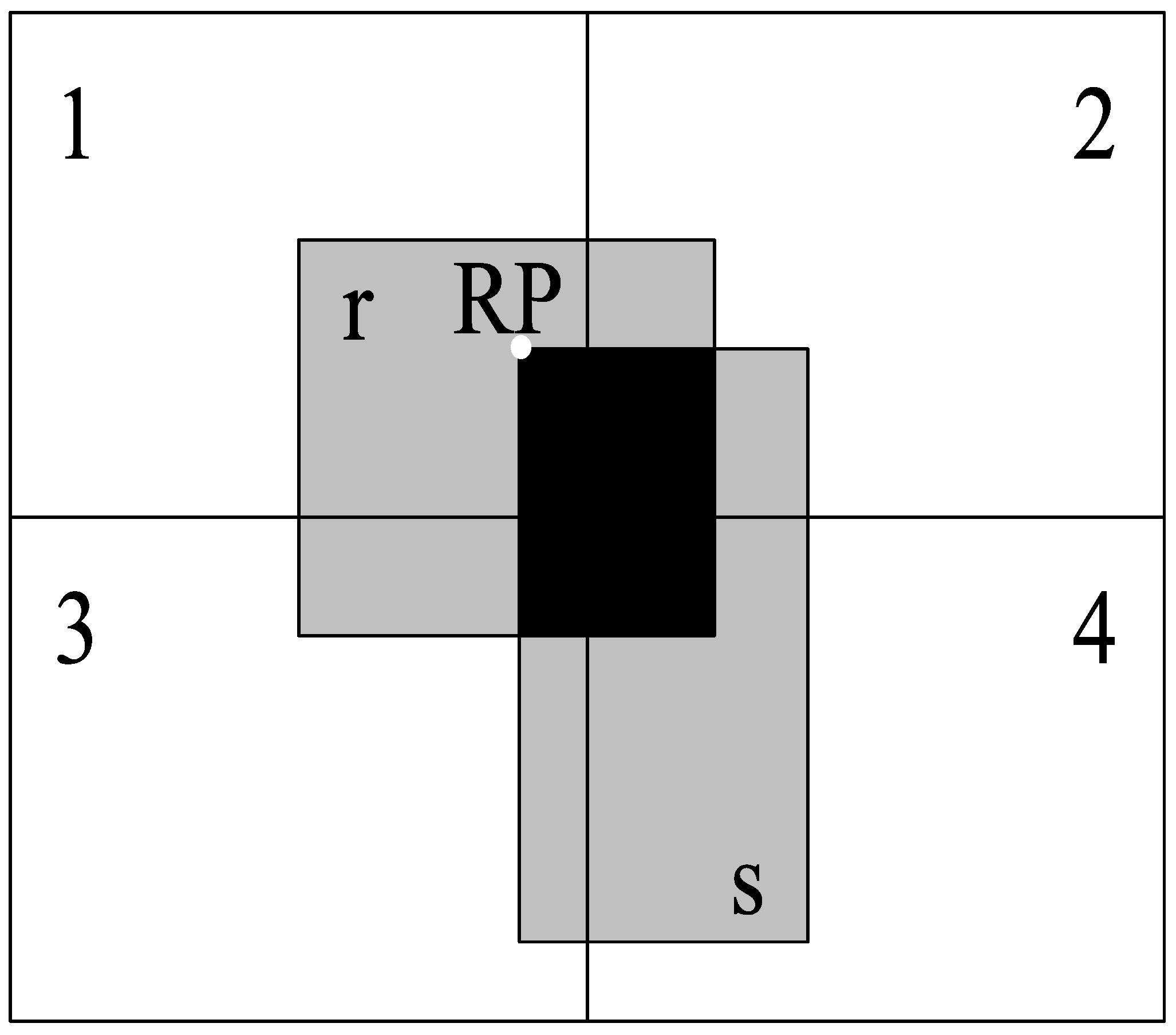If the reference point of r and s is not in the partition, the current calculation is terminated. As shown in Figure 3, the black area represents the intersect-MBR of spatial objects r and s; we define the left-top corner of the intersect-MBR as the reference point of r and s, i.e., RP. RP lies in Partition 1. Hence, although the spatial objects r and s are divided into four partitions (as stated in Section 3.1), the spatial relationship is calculated only in Partition 1. Thus, the calculations are not repeated for Partitions 2, 3 and 4.

Finally, if two spatial entities meet a predetermined spatial predicate, their ID pairs are the output, i.e., the in-memory spatial join result of the current partition.

The data storage, data flow and main processing stage of the SJS are shown in Figure 4.

4. Experiments and Evaluation

In this section, we measure the impact of cluster scale, partition number, repartition threshold value and dataset characteristics on the performance of SJS. Given the same operating environment, we compare SJS with the three spatial joins designed for MapReduce and Spark, i.e., SJMR on SpatialHadoop (SHADPOOP-SJMR), Distributed Join on SpatialHadoop (SHADOOP-DJ) [15] and SpatialSpark (SSPARK) [18]. In addition, we also compare three other in-memory spatial join algorithms for SJS: plane-sweep, quadtree index nested-loop and R-tree index nested-loop. The nested loop spatial join is the theoretical worst case of a join and shows poor performance for large datasets, and thus, we did not consider it.

4.1. Experiment Setup and Datasets

The experiments are performed with Hadoop 2.6.0 and Spark 1.0.2 running on JDK 1.7 on DELL PowerEdge R720 servers, each consisting of an Intel Xeon E5-2630 v2 2.60-GHz processor, 32 GB main memory and 500 GB SAS disk. SUSE Linux Enterprise Server 11 SP2 operating system and ext3 file system are present on each server. In order to compare the performance with that of SpatialHadoop, we deploy SpatialHadoop release Version 2.3 with Hadoop 1.2.1 on the same hardware environment described above.

The datasets used in the experiments are from Topologically-Integrated Geographic Encoding and Referencing (TIGER) and OpenStreet Map, as listed in

Table 1. Datasets.

Dataset	Abbreviation	Records	Size	Format
all ways	AWY	164,448,446 Polylines	59.55 GB	tsv
edges	ED	72,729,686 Polygons	62 GB	csv
linearwater	LW	5,857,442 Polylines	18.3 GB	csv
areawater	AW	2,298,808 Polygons	6.5 GB	csv
arealm	LM	121,960 Polygons	406 MB	csv
primaryroads	PR	13,373 Polylines	77 MB	csv

. All of the files can be downloaded from the website of SpatialHadoop [38].

We deploy the Spark projects on a Hadoop cluster and perform the execution on Hadoop YARN (next generation of MapReduce). In the case of Spark in YARN mode, executor number, executor cores and executor memory refer to the total task progression on all nodes, task threads per executor and maximum main memory allocated in each executor, respectively. All of the parameters should be preset before submitting the Spark job, which are shown in detail in

Table 2. Experiment parameters.

Experiment-Figure	Datasets	Spatial Predicate	Partitions	Nodes	Executors	Executor Cores	Executor Memory
Section 4.2-Figure 5	LW and AW	intersects	150 × 300	X-axis	nodes	series	2 GB
Section 4.3-Figure 6	LW and ED	intersects	X-axis	8	8	6	6 GB
Section 4.3-Figure 7	LW and ED	intersects	250 × 500	8	8	6	6 GB
Section 4.4-Figure 8	X-axis	intersects	200 × 400	8	8	6	6 GB
Section 4.4-Figure 9	AWY and ED	X-axis	400 × 400	8	8	6	6 GB
Section 4.5-Figure 10a	X-axis	intersects	150 × 300	8	8	6	6 GB
Section 4.5-Figure 10b	LW and AW	intersects	X-axis	8	8	6	6 GB

.

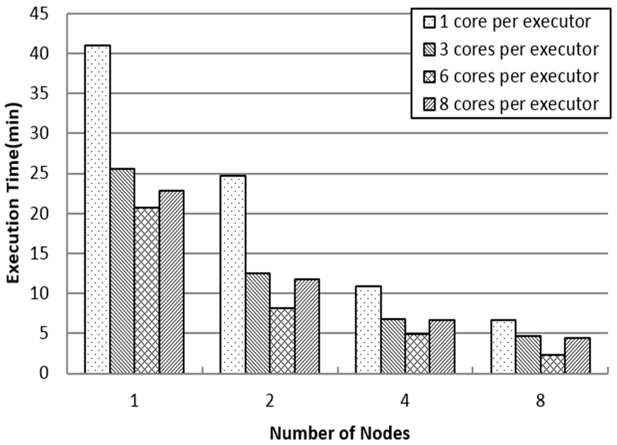
4.2. Impact of Number of Nodes and Executor Cores

Figure 5 shows the impact of the number of nodes and executor cores on SJS performance. There is a direct relationship between SJS performance and the number of nodes. When the number of executors per node is fixed at one, SJS performance improves significantly with an increase in the number of nodes. Thus, in this case, SJS shows high scalability. However, with an increase in the number of cores per executor, the execution time of SJS may not always decrease. For instance, notwithstanding the number of nodes, the execution time for eight cores per executor is significantly greater than that for six cores per executor. Hence, when the number of executors equals the number of nodes (each node runs one executor) and the cores per executor is set to six, which is equal to the CPU cores of each node, SJS performs the best. As the number of cores per executor increases, the number of tasks scheduled on a CPU also increases, thus leading to poor performance.

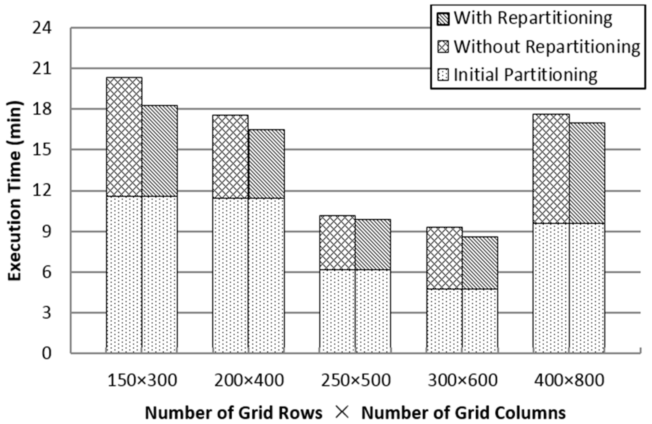
4.3. Impact of Number of Partitions and Repartitioning

As shown in Figure 6, when the number of partitions is small, there is a large amount of data in each partition, which can trigger memory overflow or larger computation time. Furthermore, as the number of partitions increases, an excessive number of duplicates can lead to unnecessary calculation. Repartitioning can refine the data size and limit the processing time of each partition to support the in-memory spatial join in a better manner. Notwithstanding the number of partitions, SJS with repartitioning can reduce total execution time by 5%–25%, without considering the initial partitioning.

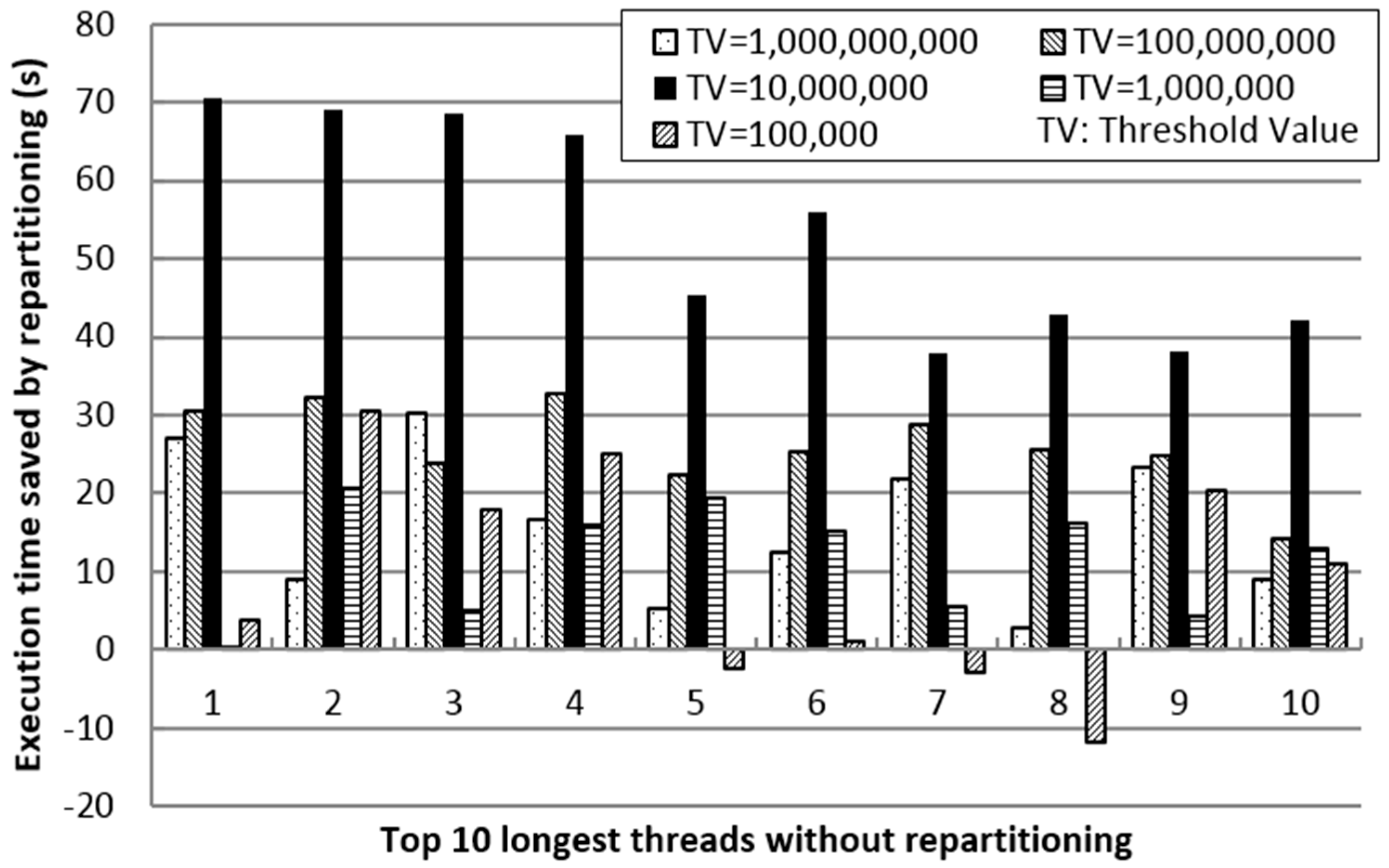
Figure 7 shows the impact of the threshold value in repartitioning on saved execution time. The negative value means the time is wasted by repartitioning; negative contributes to improve the performance. First, we sort the execution time of the processing threads (each partition is processed in one thread) of SJS without repartitioning in every node to obtain a list of the top 10 longest threads. Then, we vary TV from 100,000–1,000,000,000 in order to compare the time saved by repartitioning for each corresponding thread. From the results, we can observe that when TV is 10,000,000, significant time is saved by repartitioning. Thus, as TV decreases, the number of duplicates increases. However, as TV increases, partition refinement decreases. Hence, by efficiently reducing the execution time of the longest threads of SJS without repartitioning, in-memory repartitioning improves the performance of SJS significantly.

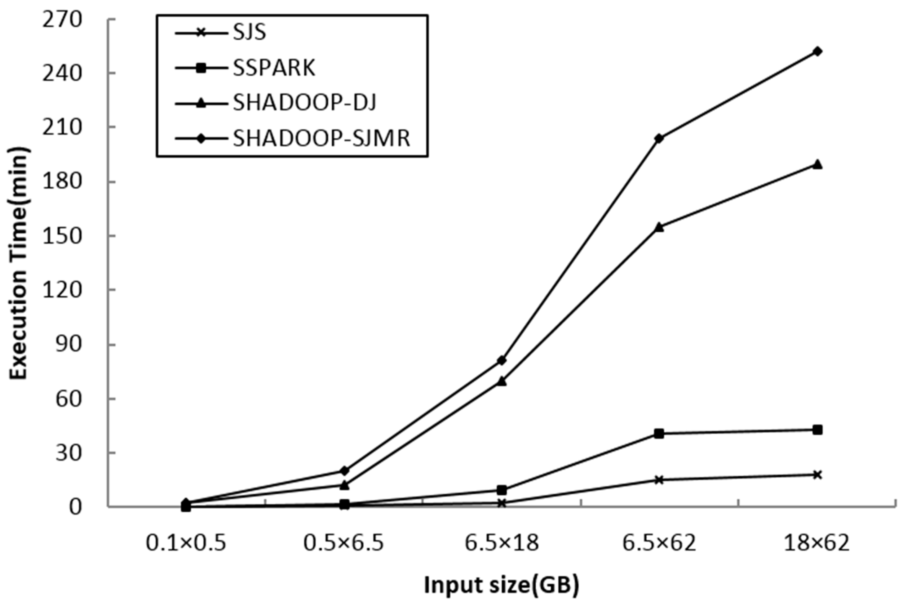
4.4. Comparison between SHADOOP-SJMR, SHADOOP-DJ, SSPARK and SJS

In order to compare the performance of other spatial join algorithms designed for MapReduce or Spark, such as SHADOOP-SJMR, SHADOOP-DJ and SSPARK, we performed a comparison test using the various dataset sizes that are listed in Section 4.1 as input. For the algorithms that run on SpatialHadoop, we measure the execution time including the preprocessing time (such as the index creation time). All of the tests are executed on the same cluster with a suitable software framework.

We vary the input dataset size from 0.1 GB × 0.5 GB to 18 GB × 62 GB. From Figure 8, it is observed that SJS’s performance is significantly better than that of the other algorithms. The results prove that SJS can manage massive spatial datasets and also deliver the best performance among the parallel spatial join algorithms.

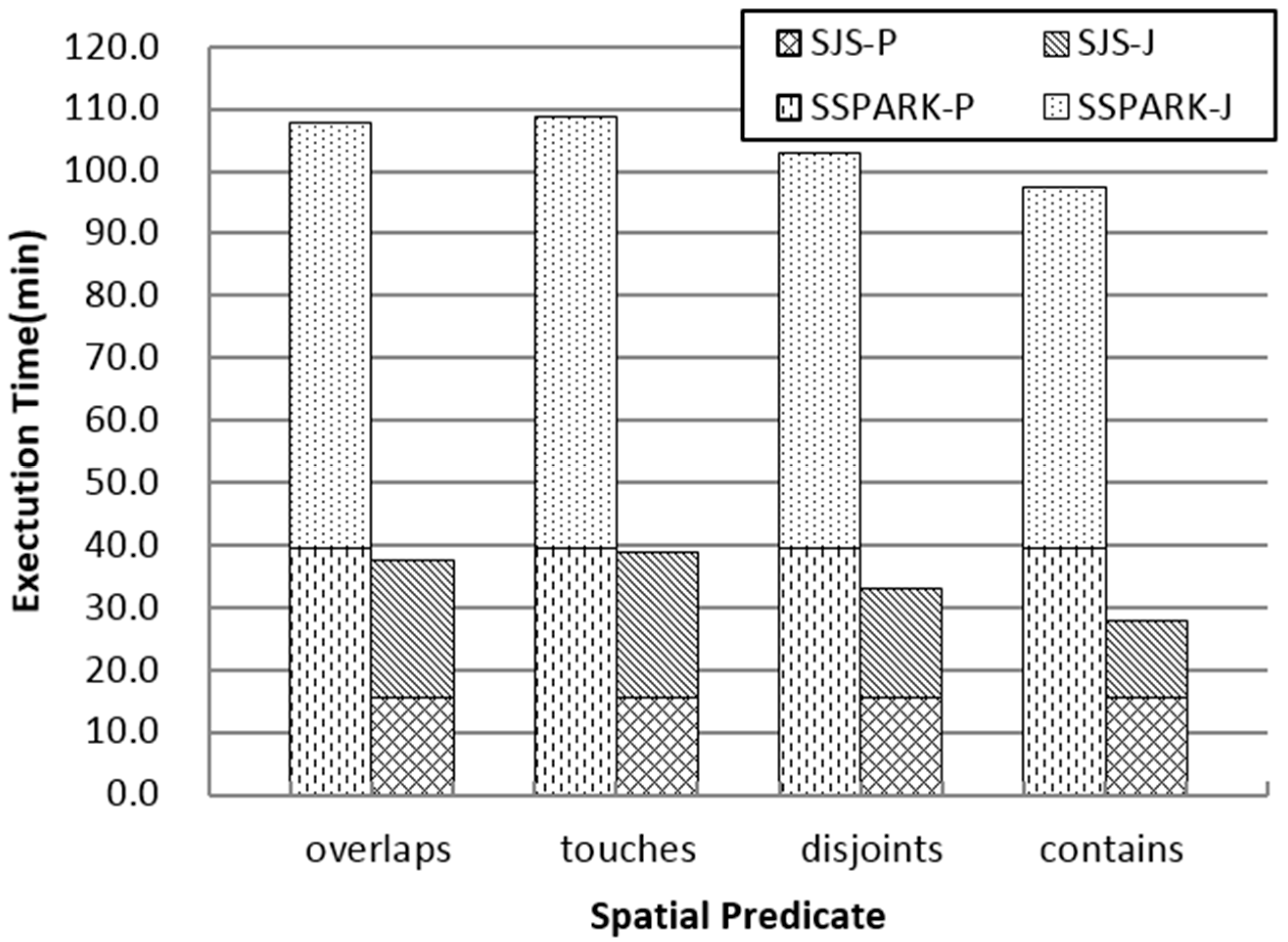
Both Hadoop-GIS and SpatialHadoop are Hadoop-based and write their intermediate results to disk, and thus, we make a detailed comparison with SpatialSpark. Given that SpatialSpark uses Java Topology Suite (JTS) as the topological analysis library, we performed the comparison test using various spatial predicates, such as overlaps, touches, disjoints and contains. In the case of SpatialSpark, we use the sort tile partition method, set the sample ratio at 0.01, and the others are same as SJS.

Since transformations in Spark only execute when an action occurs, the actions in SJS are only “groupBy” in the partition phase and “saveAsTextFile” (“distinct” in SSPARK) in the last. Thus, we separate both SJS and SSPARK mainly in two phases, one is the partition phase; the other is the partition join and local join phase (including the repartition phase in SJS).

As shown in Figure 9, because SJS uses grid partition, which is more efficient than SATO in SSPARK, the execution time in the partition and partition join phase of SJS is significantly reduced. Given that (1) the repartition phase in SJS limits the processing time of each partition, which is suitable for the task schedule strategy of Spark; (2) the duplicates are avoided before refinement; and (3) the R*-tree local join algorithm in SJS outperforms R-tree nested-loop join in SpatialSpark, SJS performs better than SpatialSpark. Figure 9 also shows that both SpatialSpark and SJS support various topological analyses on large spatial datasets, and different spatial predicates obviously affect the final performance.

4.5. Performance Comparison between Various in-Memory Spatial Join Algorithms for SJS

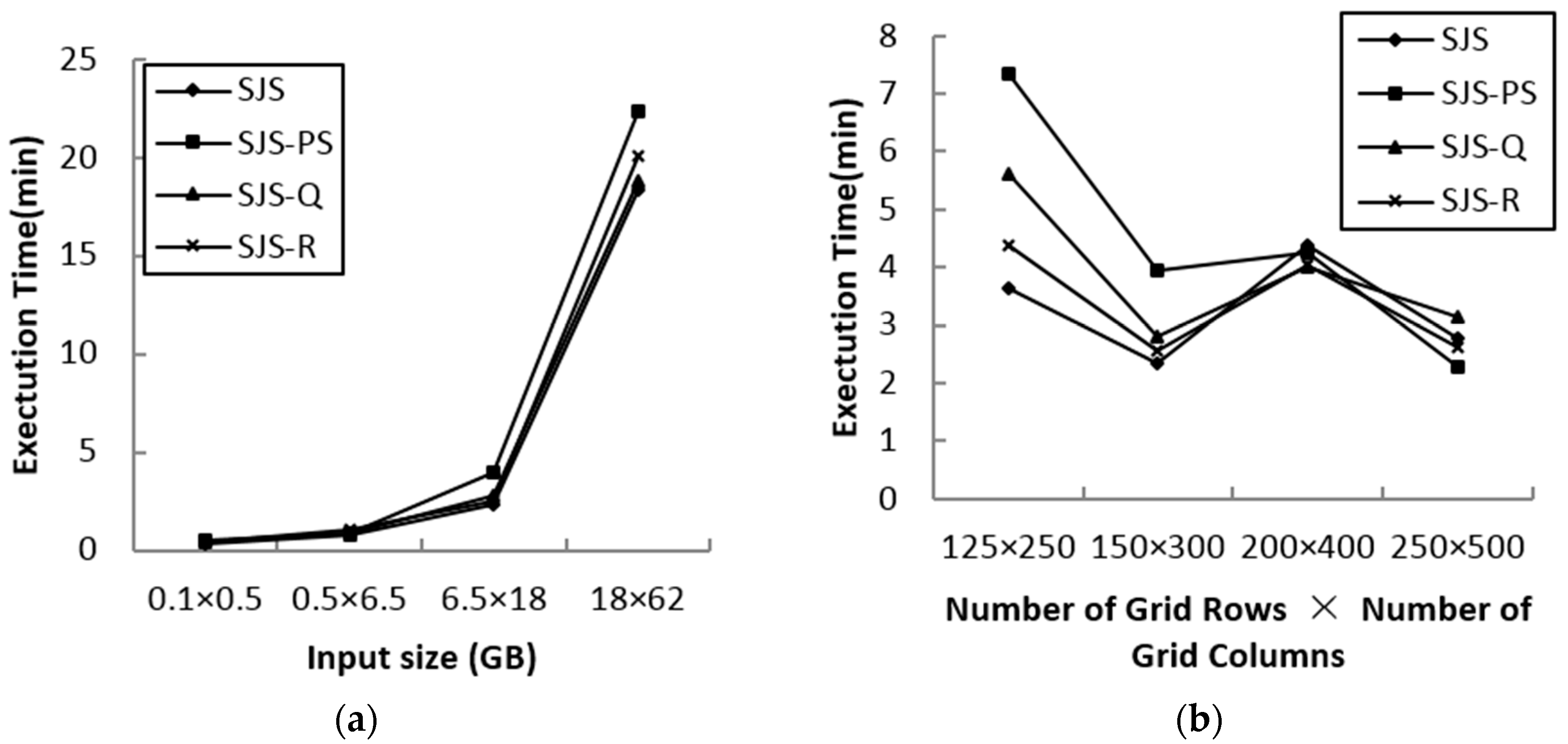
In order to test the performance of various in-memory join algorithms used in the SJS in-memory join phase, Plane-Sweep (SJS-PS), Quadtree index nested-loop join (SJS-Q) and R-tree index nested-loop join (SJS-R) are compared. Figure 10a shows the performance comparison results for various input data sizes. Figure 10b shows the performance comparison results for various grid sizes using linearwater (LW) and areawater (AW) as the input datasets.

We can observe that the default R*-tree index nested-loop join has the best performance for all input and grid sizes in most cases. The size of each partition is suitable for every in-memory spatial join method after repartitioning refinement; thus, although the data scale is large, the performance difference between the methods is smaller than the approaches in [23].

5. Conclusions and Future Work

Recent advances in geocomputation techniques greatly enhance the abilities of spatial and sustainability scientists to conduct large-scale data analysis. Such large-scale data analytics will stimulate the development of new computational models. In turn, these newly-developed methods get adopted in real-world practice, forming a positive feedback loop [39]. Rigorous spatial analysis and modeling of socioeconomic and environmental dynamics opens up a rich empirical context for scientific research and policy interventions [40]. A robust spatial join can serve as a fundamental analytical power to understand how everything is related and to what extent, such as how a firm’s location is related to a specific site in a large national dataset [41] or disaster risk related to multiple spatially-related factors [42,43]. In this study, we proposed and described SJS, a high-performance spatial join algorithm with Spark. SJS can be deployed easily on large-scale cloud clusters, and it significantly improves the performance of spatial join on massive spatial datasets. This research proves that the availability of large-size geo-referenced datasets along with the high-performance computing technology can raise great opportunities for sustainability research on whether and how these new trends in data and technology can be utilized to help detect the associated trends and patterns in the human-environment dynamics. In other words, such computing power allows for the measuring and monitoring of sustainability in a very large datasets and can respond within a very short time period. The iterative computation characteristics of Spark make it possible to perform in-memory parallel spatial join with minimal disk access. In particular, the calculation-evaluating-based in-memory repartition technology evaluates the CPU cost of each partition, thus differing from the repartitioning method that considers only the memory or a single dataset; hence, the result is more suitable for in-memory spatial join in Spark. The reference point method that we implemented in Spark was adopted in order to avoid duplicates instead of the built-in distinct transformation, which eliminates repetitive calculations. Benefitting from the high space utilization and retrieval speed of R*-tree, each partition executes a high-performance index nested-loop spatial join in parallel. Based on extensive evaluation of real datasets, we demonstrate that SJS performs significantly better than earlier Hadoop-like spatial join approaches.

The coupling relationship between multiple driving forces in the spatial context has been heatedly debated in a variety of environmental studies [44]. This pilot study demonstrated the promising feature of high-performance computing on the solution of large-scale spatial join to explore geographical relationships. In future work, we will improve the accuracy of the calculation evaluating model and apply recent in-memory spatial join methods, such as TOUCH, to Spark in order to maximize local join performance. In addition, the temporal dimension will also be added to investigate spatiotemporal join, and high-dimensional geographic objects will also be explored. It warrants noticing that an efficient 2D spatial index, such as R*-tree, will no longer be suitable in the high dimensional space.