The Multilevel Index Decomposition of Energy-Related Carbon Emission and Its Decoupling with Economic Growth in USA

Abstract

The United States of America is not only an important energy consuming country, but also in the dominant position of energy for many years. As one of the two largest emitters, the US has always been trying to register a decline in energy-related CO₂. In order to make a further analysis of the phenomenon, we choose a new decoupling analysis with the multilevel logarithmic mean Divisia index (LMDI) method. This study examined the contribution of factors influencing energy-related carbon emissions in the United States of America during 1990–2014, quantitatively analyzed decoupling indicators of economic development and environmental situations. As is indicated in the results, economy development and activities have a significant effect in increasing carbon emission, however, measures of energy optimization such as the improvement of energy efficiency has played a crucial role in inhibiting the carbon dioxide emission. Furthermore, as is indicated in decoupling relationship, “relative decoupling” and “no decoupling” are the main states during the examined period. In order to better investigate the long-run equilibrium relationship between total carbon dioxide emissions of each effect and the relationship between CO₂ emissions and economic growth, on the basis of a static decomposition analysis, we applied a dynamic analysis method-cointegration test. At last, recommendations and improvement measures aiming at the related issues were put forward.

1. Introduction

Recently, how to decouple economic growth from carbon emission has become a hot issue [1,2,3,4,5,6,7]. The United States has been the world’s first largest economy and second largest emitter of CO₂. According to the International Energy Agency, the US reduced energy-related carbon emissions more than any country or region, falling 7.7% during 2006–2011 [8]. It also should be noted that the US economy kept growing during the same time. In this paper, we try to figure out the factors and system that influence the energy-related carbon emissions, and then effective measures and policies for decoupling economic growth and carbon emissions are developed based on the analysis of driving factors.

There are many studies on CO₂ emissions, however, most of the studies before tend to focus more on the impacts brought by the change of CO₂ emissions [9,10,11,12,13,14,15,16] and how the greenhouse effect influences economic activities [17,18,19,20,21,22,23]. As for research methods, generally speaking, there are two approaches to the research: econometric analysis [24,25,26,27,28,29,30,31,32,33,34,35,36,37,38] and decomposition methods [39,40,41,42,43,44]. By using the cointegration analysis method, Ozturk [45] explored the relationship between economic growth and carbon dioxide emissions in Turkey. Diakoulaki [46] analyzed the driving forces of CO₂ emissions from the perspective of manufacturing sector in European Union and González [47] studied from electricity sector. In order to analyze the influencing factor of carbon emissions in Beijing–Tianjin–Hebei economic band of China quantitatively, Wang used decomposition method and got a promising result [22]. Among various index decomposition analysis methods of the IDA model, logarithmic mean Divisia index method was considered the most suitable and widely applied [48,49]. In addition, studies on decoupling tended to focus more on the exploration of the link between human economic activities and environmental changes [50,51,52], using Tapio method [53].

Based on the previous studies, this article analyzed the decomposition of energy-related carbon emissions in the USA during 1990–2014, applying the LMDI method. In order to probe the relationship between economic activities and carbon dioxide emissions better, we applied a novel decoupling index, demonstrating the decoupling status influenced by different effects in four aspects. The reason why the period was chosen was that it witnessed rapid economic development in this stage in the USA, as a consequence, it was most likely to bring about changes in carbon dioxide emissions. Furthermore, this paper introduced a new decoupling method to illuminate the relationship between economic growth and carbon emissions.

2. Methodologies and Date Definitions

2.1. Methodologies

2.1.1. Index Decomposition Analysis

As is shown in the Kaya identity, there are four principal factors affecting carbon emissions, based on expanded Kaya identity [54,55] and the researches of Ang [56,57], this study applied both additive LMDI and multiplicative LMDI to show how the four driving factors affect the carbon dioxide emissions. The aggregate carbon dioxide emissions in America can be evaluated as follows:

$$C={\displaystyle \sum _i{C}_i}={\displaystyle \sum _{i}P\times \frac{Q}{P}}\times \frac{E}{Q}\times \frac{E_i}{E}\times \frac{C_i}{E_i}={\displaystyle \sum _{i}P\times G\times I\times }{M}_i\times F_i$$

(1)

where C is the total energy-related carbon dioxide emissions, P is the total population (10⁴ person), G refers to total economic activity condition and we choose gross domestic product (GDP) as the indicator (constant US dollars of 2005), E is total primary energy consumption (Mtce), E_i is energy consumption of fuel i (Mtce); Q/P is per-capita GDP, I = E/Q is the energy intensity of GDP (we use primary energy as a proxy of final energy consumption), M_i = E_i/E is denotes the energy share of the fuel i, F_i = C_i/E_i is carbon dioxide emissions coefficient of fossil energy.

According to the LMDI method [58,59], the carbon dioxide emission from year 0 to year t can be expressed in additive and multiplicative forms by the following Equations (2) and (3):

$$\Delta C=C^T-C^0=\Delta C_{pop}^T+\Delta C_{act}^T+\Delta C_{int}^T+\Delta C_{mix}^T+\Delta C_{fac}^T$$

(2)

$$D=C^T/C^0=D_{pop}{D}_{act}{D}_{int}{D}_{mix}{D}_{fac}$$

(3)

where $\Delta C$ refers to total changes in carbon emissions from year 0 to year T, which can be further decomposed to five indictors: $\Delta C_{pop}$ (the effect of population), $\Delta C_{act}$ (the effect of human economic activities effect), $\Delta C_{int}$ (the effect of energy intensity), $\Delta C_{mix}$ (the effect of energy mix), $\Delta C_{fac}$ (the effect of carbon dioxide emission factor).

$D$ is the total carbon dioxide growth rate, which can be decomposed to five aspects: $D_{pop}$ (population effect), $D_{act}$ (human economic activities effect), $D_{int}$ (energy intensity effect), $D_{mix}$ (energy-mix effect), $D_{fac}$ (carbon emission effect). Total effect can be described in two ways: additive decomposition and multiplicative decomposition.

Additive decomposition is as follows:

$$\Delta C_{pop}^T={\displaystyle \sum _i}\frac{C_i^T-C_i^0}{\ln C_i^0-\ln C_i^0}\ln \frac{P^T}{P^0}$$

(4)

$$\Delta C_{act}^T={\displaystyle \sum _i}\frac{C_i^T-C_i^0}{\ln C_i^0-\ln C_i^0}\ln \frac{G^T}{G^0}$$

(5)

$$\Delta C_{int}^T={\displaystyle \sum _i}\frac{C_i^T-C_i^0}{\ln C_i^0-\ln C_i^0}\ln \frac{I^T}{I^0}$$

(6)

$$\Delta C_{mix}^T={\displaystyle \sum _i}\frac{C_i^T-C_i^0}{\ln C_i^0-\ln C_i^0}\ln \frac{M^T}{M^0}$$

(7)

$$\Delta C_{fac}^T={\displaystyle \sum _i}\frac{C_i^T-C_i^0}{\ln C_i^0-\ln C_i^0}\ln \frac{F^T}{F^0}$$

(8)

Multiplicative decomposition is as follows:

$$D_{pop}=\exp ({\displaystyle \sum _i\frac{(C_i^T-C_i^0)/(\ln C_i^T-\ln C_i^0)}{(C^T-C^0)/(\ln C^T-\ln C^0)}}\ln \frac{P^T}{P^0}$$

(9)

$$D_{act}=\exp ({\displaystyle \sum _i\frac{(C_i^T-C_i^0)/(\ln C_i^T-\ln C_i^0)}{(C^T-C^0)/(\ln C^T-\ln C^0)}}\ln \frac{G^T}{G^0}$$

(10)

$$D_{int}=\exp ({\displaystyle \sum _i\frac{(C_i^T-C_i^0)/(\ln C_i^T-\ln C_i^0)}{(C^T-C^0)/(\ln C^T-\ln C^0)}}\ln \frac{I^T}{I^0}$$

(11)

$$D_{mix}=\exp ({\displaystyle \sum _i\frac{(C_i^T-C_i^0)/(\ln C_i^T-\ln C_i^0)}{(C^T-C^0)/(\ln C^T-\ln C^0)}}\ln \frac{M^T}{M^0}$$

(12)

$$D_{fac}=\exp ({\displaystyle \sum _i\frac{(C_i^T-C_i^0)/(\ln C_i^T-\ln C_i^0)}{(C^T-C^0)/(\ln C^T-\ln C^0)}}\ln \frac{F^T}{F^0}$$

(13)

2.1.2. The Decoupling Measurement between CO₂ Emissions and Economic Growth

There are many index decomposition methods, LMDI is a useful method which is widely used. Generally speaking, the decoupling index can be measured by the ratio defined by Tapio [53], based on the LMDI results, we analyzed the decoupling elasticity from five aspects:

$$\begin{gathered} \epsilon =\frac{\Delta C/C^T}{\Delta G/G^T}=\frac{\Delta C_{pop}/C^T}{\Delta G/G^T}+\frac{\Delta C_{act}/C^T}{\Delta G/G^T}+\frac{\Delta C_{int}/C^T}{\Delta G/G^T}+\frac{\Delta C_{mix}/C^T}{\Delta G/G^T}+\frac{\Delta C_{fac}/C^T}{\Delta G/G^T} \\ ={\mathsf{\epsilon }}_{pop}+{\mathsf{\epsilon }}_{act}+{\mathsf{\epsilon }}_{int}+{\mathsf{\epsilon }}_{mix}+{\mathsf{\epsilon }}_{fac} \end{gathered}$$

(14)

where $\Delta C/C$ refers to energy-related CO₂ emission changes ratio, $\Delta G/G$ refers to the ratio of GDP changes. Where ε represents to the decoupling elasticity index, ${\mathsf{\epsilon }}_{pop}$, ${\mathsf{\epsilon }}_{act}$, ${\mathsf{\epsilon }}_{int}$, ${\mathsf{\epsilon }}_{mix}$, ${\mathsf{\epsilon }}_{fac}$ are the decoupling elasticity values of population effect, economic activities effect, energy intensity effect, energy mix effect, and CO₂ emission factor effect.

In order to probe the decoupling status in a convenient and intuitive way, a novel decoupling index is proposed. In this article, based on the additive decomposition results of energy-related CO₂ emission changes, we combine the LMDI with a decoupling index which was advanced by Diakoulaki [46] and Vehmas [60].

America’s economy has developed rapidly during the study period, causing the increase of carbon dioxide emissions. Meanwhile, thanks to some government measures such as improving energy efficiency, setting tight restrictions on the amount of energy used, and optimizing energy mix, the carbon dioxide emissions, to some degree, can be reduced. In order to show the total inhibiting effect, we use the equation as follows:

$$\Delta C_T=\Delta C^T-\Delta C_{act}^T=\Delta C_{pop}^T+\Delta C_{int}^T+\Delta C_{mix}^T+\Delta C_{fac}^T$$

(15)

where $\Delta C_T$ is the total inhibiting effect on CO₂ emission. In order to obtain a further understanding of the influencing mechanism, we apply a new decoupling measurement between CO₂ emissions and economic growth. The decoupling index presents intuitive relationship between environmental impacts and economic development in different aspects.

The decoupling index is defined as follows:

$${\delta }_T=-\frac{\Delta C_T}{\Delta C_{act}^t}=-\frac{\Delta C_{pop}^T}{\Delta C_{act}^T}-\frac{\Delta C_{int}^T}{\Delta C_{act}^T}-\frac{\Delta C_{mix}^T}{\Delta C_{act}^T}-\frac{\Delta C_{\text{fac}}^T}{\Delta C_{act}^T}={\mathsf{\delta }}_{pop}^T+{\mathsf{\delta }}_{int}^T+{\mathsf{\delta }}_{mix}^T+{\mathsf{\delta }}_{fac}^T$$

(16)

where ${\mathsf{\delta }}_T$ refers to the total decoupling index, and ${\mathsf{\delta }}_{pop}$, ${\mathsf{\delta }}_{int}$, ${\mathsf{\delta }}_{mix}$, ${\mathsf{\delta }}_{fac}$ indicate the population, the effect of energy intensity, energy mix effect and carbon dioxide emission factor on the decoupling between carbon dioxide emissions and economy.

If ${\mathsf{\delta }}_T$ ≥ 1, it refers to a strong decoupling effect. In other words, the total CO₂ emissions inhibiting effect is more significant than the effect of economic growth. If 0 < ${\mathsf{\delta }}_T$ < 1, it indicates the relative decoupling effect, showing that the CO₂ emission inhibiting effect is weaker than the effect of economic growth. If ${\mathsf{\delta }}_T$ ≤ 0, it indicates no decoupling effect representing that the possible inhibiting factors cannot reduce CO₂ efficiently, on the contrary, it brings about an increase. The results can help us to probe the relative contribution of each factor to the overall decoupling progress.

2.2. Date Definitions

Data for this study period (from 1990 to 2014) was acquired primarily from the World Bank [61]. Energy data including the total primary energy consumption, CO₂ emissions and the rate of every energy form data came from the World Bank [61] and BP Statistical Review of World Energy [62] The gross domestic product (GDP) and the population data was also obtained from the World Bank [61]. Economic data measured by GDP was taken in constant prices of 2005 to eliminate the error caused by inflation.

3. Results and Discussion

3.1. The Trajectory of CO₂ Emissions in USA

As is shown in Figure 1, per capita CO₂ emissions and CO₂ emissions intensity can be analyzed in two stages: 1990–2005 and 2006–2014. In the first stage, the change of per capita CO₂ emissions was not very significant, but the change of CO₂ emission intensity decreased a lot. In the second stage, per capita CO₂ emissions decreased sharply but CO₂ emission intensity has a smooth and moderate decline. In general, the average annual growth rate of CO₂ emission intensity was −2.06%, however, in the first stage, the average annual growth rate of CO₂ emission intensity was −1.95%. The average annual growth rate of per capita CO₂ emissions was −0.65%, disappointingly, the average annual growth rate of per capita CO₂ emissions in stage 1 was −0.002%. In the second stage, the average annual growth rate of CO₂ emission intensity was −2.03% and the average annual growth rate of per capita CO₂ emissions was −1.67%.

Figure 2 shows that total CO₂ emission was on the rise and per capita CO₂ emission did not show a decreasing trend at first while dropped in next phase. Total CO₂ emissions, on the whole, were on the rise. While per capita CO₂ emissions increased first and then decreased. As stated above, it can be divided into two stages. During the first stage (1990–2005), in general, per capita CO₂ emissions were on the rise, however, in stage 2, it appeared a decreasing trend. When it comes to total CO₂ emissions, although there was a short growth, in general, it could be concluded that it decreased.

3.2. Decomposition Results of CO₂ Emissions

3.2.1. The Additive Decomposition Results of CO₂ Emissions Changes

Figure 3 indicates the changes of carbon dioxide emission of different factors (ΔC_pop, ΔC_act, ΔC_int, ΔC_mix, ΔC_fac), and the changes of the CO₂ emissions expresses in the form of a line chart. From 1990 to 2014, various factors has different effects in America. Among the five factors, the population effect and activity effect played a positive role, however, intensity effect contributed to decreasing the CO₂ emissions. The other two factors varied from year to year. From the perspective of effect level, population effect and intensity effect made more contributions to the carbon emissions, mix effect was relatively weak.

In the first phase, although there is a certain amount of CO₂ emissions fluctuations, but the trend is rising, anyway, in stage 2, in a certain range of fluctuations, the overall trend is declining.

In general, economic activity effect contributed to decrease the carbon emissions during the study period. In the first stage, economic activity effect is the most important impact, however, in the second half of the first stage, the effect became more significant. In the first stage, the total change of CO₂ emissions was 1656.33 Mt. Generally speaking, in stage 1, the economic activities effect increased carbon emissions, in the second phase, changes of economic activities effect on carbon dioxide emissions experienced a sharp decline at first and then rebounded. On the whole, the effect on carbon dioxide emissions decreased in the second stage. In addition, the change of CO₂ emissions was 1826.26 Mt during the study period.

Population effect influence degree in the first stage experienced some fluctuations, but overall, the influence degree decreased, during the first study phase, the carbon dioxide emissions changed by 948.70 Mt. During the next period, population effect contributed less with some fluctuations. Overall, the effect caused by the population weakened in 2014 compared with 1990 with the change of 1311.35 Mt.

Intensity effect played a negative role in the carbon emissions, in other words, intensity effect helped to decrease the carbon emissions. Furthermore, in phase 1, the effect caused by energy intensity of GDP was on the rise, causing the carbon emissions declined by 1605.35 Mt. The effect weakened during the second stage. On the whole, it played a more and more important role during the study period. When it comes to the share of intensity effect as a factor, it increased at first while there was a decline in stage 2, and despite of some fluctuations, it grew on the whole, with the amount of 4114.62 Mt.

Energy-mix effect did not show a significant impact on carbon dioxide emissions even though it contributed to increase the emissions. In stage 1, the influence did not change much and it increased a little in the second phase. However, in phase 2, with the adjustment of energy mix, it shows a step to independence from traditional fossil energy. The most efficient way to reduce carbon dioxide emissions is to increase non-fossil energy consumption such as nuclear, hydro power and other renewable sources. As a result, phase 2 shows a more significant impact than the former stage.

Influence cause by energy penetration effect was complex, that’s say, sometimes it played a positive role but sometimes are not. When it comes to the share of energy penetration effect as a factor, it did not change at first while there was little increase next. When it comes to the share of energy penetration effect as a factor, it changed little with only the increase of 2.98 Mt at first, however, while it increased next, during the whole study period, the carbon dioxide emissions decreased by 260.44 Mt.

As is shown in

Table 1. Share of each factor’s change rate (%).

Time Period	ΔCpop	ΔCact	ΔCint	ΔCmix	ΔCfac
1990–1991	31.1523	32.8800	0.9570	15.5715	19.4392
1991–1992	23.6153	35.8731	32.3751	5.3448	2.7918
1992–1993	31.4543	33.1592	14.9793	3.3631	17.0442
1993–1994	18.1975	40.5408	31.6274	1.3629	8.2713
1994–1995	25.5246	31.9785	11.9563	19.9365	10.6041
1995–1996	25.8559	56.9428	10.0439	3.5547	3.6027
1996–1997	12.2844	32.5007	36.7013	6.7527	11.7610
1997–1998	13.9543	38.1625	44.5112	1.1491	2.2229
1998–1999	12.9858	38.7924	32.7986	5.8562	9.5670
1999–2000	15.9878	41.6357	24.9462	8.3924	9.0379
2000–2001	20.9767	0.3919	70.6941	5.4686	2.4687
2001–2002	29.9921	27.2369	8.1880	25.4090	9.1740
2002–2003	14.5511	32.3132	40.9228	7.0152	5.1978
2003–2004	15.3264	46.2096	28.1866	0.8786	9.3988
2004–2005	13.5676	34.8683	46.9220	3.5683	1.0738
2005–2006	13.5342	23.4041	47.1666	6.9561	8.9389
2006–2007	44.1762	37.7118	5.5073	5.6186	6.9861
2007–2008	18.4496	24.1462	37.1578	11.9808	8.2656
2008–2009	8.6553	36.4459	22.0188	19.6517	13.2282
2009–2010	19.9643	39.7433	24.5132	10.6869	5.0923
2010–2011	12.0115	12.9448	38.2849	23.7540	13.0048
2011–2012	7.7047	15.4375	48.2081	13.3110	15.3387
2012–2013	25.2346	47.9798	18.0334	1.7039	7.0482
2013–2014	18.1164	39.4498	26.8782	8.1075	7.4481

, economic activities and energy intensity were the major factors that influencing the CO₂ emissions even though energy intensity effect had a negative effect. Furthermore, population and emissions factor also played a relatively important role, but the energy mix did not show significant influence.

3.2.2. The Multiplicative Decomposition Results of CO₂ Emissions Changes

In order to make the results more accurate, we further exploration with the method of multiplicative decomposition. From the results above we can conclude that both population and economic activities played a role in increasing carbon dioxide emissions, On the contrary, the energy intensity contributed to decrease the CO₂ emissions. In addition, energy mix varied from year to year, but in general it had a positive effect.

To further refine dynamic comparative analysis, multiplicative decomposition is applied. Compared with addictive LMDI decomposition, the multiplicative LMDI decomposition method can rationalize the driving factors of CO₂ emissions better. The multiplicative decomposing result shown in

Table 2. Multiplicative LMDI decomposition of CO₂ emissions.

Time Period	$D_{\mathit{p}\mathit{o}\mathit{p}}$	$D_{\mathit{a}\mathit{c}\mathit{t}}$	$D_{\mathit{i}\mathit{n}\mathit{t}}$	$D_{\mathit{m}\mathit{i}\mathit{x}}$	$D_{\mathit{f}\mathit{a}\mathit{c}}$	$D_{\mathit{t}\mathit{o}\mathit{t}}$
1990–1991	1.0047	0.9950	0.9996	1.0070	1.0002	1.0066
1991–1992	1.0140	1.0213	0.9812	1.0031	1.0042	1.0235
1992–1993	1.0133	1.0140	0.9937	1.0014	0.9919	1.0142
1993–1994	1.0123	1.0277	0.9789	0.9991	0.9988	1.0163
1994–1995	1.0120	1.0150	0.9944	0.9907	0.9955	1.0075
1995–1996	1.0117	1.0260	0.9955	1.0016	1.0013	1.0363
1996–1997	1.0121	1.0324	0.9647	1.0066	0.9945	1.0090
1997–1998	1.0117	1.0324	0.9635	1.0010	1.0071	1.0145
1998–1999	1.0115	1.0349	0.9714	0.9948	0.9960	1.0076
1999–2000	1.0112	1.0294	0.9828	1.0059	1.0073	1.0365
2000–2001	1.0099	0.9998	0.9672	1.0026	0.9999	0.9791
2001–2002	1.0093	1.0085	0.9975	0.9922	0.9934	1.0007
2002–2003	1.0086	1.0193	0.9761	1.0042	1.0046	1.0123
2003–2004	1.0093	1.0283	0.9831	0.9995	1.0014	1.0212
2004–2005	1.0093	1.0240	0.9686	1.0024	1.0041	1.0075
2005–2006	1.0097	1.0168	0.9670	0.9951	0.9979	0.9857
2006–2007	1.0096	1.0082	0.9988	1.0012	0.9989	1.0167
2007–2008	1.0095	0.9877	0.9811	0.9939	0.9971	0.9695
2008–2009	1.0088	0.9638	0.9779	0.9803	0.9845	0.9177
2009–2010	1.0084	1.0168	1.0103	1.0045	0.9996	1.0402
2010–2011	1.0077	1.0083	0.9759	0.9850	0.9892	0.9661
2011–2012	1.0076	1.0153	0.9536	0.9873	0.9850	0.9487
2012–2013	1.0075	1.0144	1.0054	0.9995	1.0021	1.0291
2013–2014	1.0074	1.0162	0.9891	0.9968	0.9970	1.0063

clearly reveals the change of carbon dioxide emissions and provides more ways to impose restrictions on carbon emissions. On the whole, population factor, economy activity factor, and the energy mix effect made a contribution to increasing aggregate CO₂ emissions, nevertheless, the energy intensity played a negative role on the emissions. However, carbon emission effect varied from year to year. It is worth mentioning that economy activities factor played a negative role in curbing the carbon dioxide emission was the stage that economic recession took place.

3.3. The Decoupling Results

3.3.1. Decoupling Elasticity

Decoupling elasticity value of different factors based on the LMDI method demonstrates the contribution to decoupling of each effect. As is shown in

Table 3. The Decoupling elasticity value based on decomposition factors.

Time Period	${\epsilon }_{\mathit{p}\mathit{o}\mathit{p}}$	${\epsilon }_{\mathit{a}\mathit{c}\mathit{t}}$	${\epsilon }_{\mathit{i}\mathit{n}\mathit{t}}$	${\epsilon }_{\mathit{m}\mathit{i}\mathit{x}}$	${\epsilon }_{\mathit{f}\mathit{a}\mathit{c}}$
1990–1991	−16.9856	17.9277	0.5218	8.4903	10.5991
1991–1992	0.3780	0.5741	−0.5182	0.0855	−0.0447
1992–1993	0.4613	0.4863	−0.2197	0.0493	0.2500
1993–1994	0.2965	0.6605	−0.5153	−0.0222	−0.1348
1994–1995	0.4236	0.5306	−0.1984	−0.3308	−0.1760
1995–1996	0.2941	0.6476	−0.1142	0.0404	0.0410
1996–1997	0.2609	0.6902	−0.7794	0.1434	0.2498
1997–1998	0.2567	0.7021	−0.8189	0.0211	−0.0409
1998–1999	0.2418	0.7224	−0.6108	−0.1091	−0.1782
1999–2000	0.2655	0.6914	−0.4143	0.1394	0.1501
2000–2001	0.9869	−0.0184	−3.3260	0.2573	0.1161
2001–2002	0.5043	0.4580	−0.1377	−0.4272	−0.1543
2002–2003	0.2987	0.6634	−0.8401	0.1440	0.1067
2003–2004	0.2391	0.7209	−0.4397	−0.0137	−0.1466
2004–2005	0.2694	0.6924	−0.9317	0.0709	0.0213
2005–2006	0.3540	0.6122	−1.2337	−0.1820	−0.2338
2006–2007	0.5102	0.4355	−0.0636	0.0649	−0.0807
2007–2008	−3.1003	4.0576	6.2441	2.0133	1.3890
2008–2009	−0.3024	1.2734	0.7693	0.6866	0.4622
2009–2010	0.3142	0.6256	0.3858	0.1682	0.0802
2010–2011	0.4626	0.4986	−1.4746	−0.9149	−0.5009
2011–2012	0.3305	0.6621	−2.0676	−0.5709	−0.6579
2012–2013	0.3351	0.6371	0.2395	−0.0226	0.0936
2013–2014	0.3031	0.6600	−0.4497	−0.1356	−0.1246

, economic activities and energy intensity, two major factors contributed to an increasing trend of CO₂ emissions. Conversely, energy intensity effect had a negative effect. Furthermore, energy intensity effect also played a relatively important role. But the energy mix did not show significant influence compared with other influencing factors.

In general, the decoupling elasticity value of economic activities effect is the most significant among the five factors, as a result, we use the decoupling index to probe the decoupling more deeply. The eighth economic crisis after the war from 1990, first serious shock since the 1990s, influenced decoupling elasticity value of every effect, especially the population effect and human economic activities effect. Energy intensity effect had a curbing impact in most years, in other words, it contributed to the decrease of carbon dioxide emissions and showed a positive effect on the health relationship between the development of economy and environmental issues. In addition, the ratio of every factor not only shows different impacts for the reason that share of each factor’s change rate of CO₂ emissions but also represent the proportion of each factor’s elasticity value, in other words, the decoupling elasticity value can be the supplement to the previous decomposition ratio analysis of each effect. For example, human economic activities effect is not only the most significant influencing factor of CO₂ emissions as is shown in Table 1 but also a key impact affecting decoupling elasticity value. Moreover, decoupling elasticity value can reflect the deep-seated influencing system of different effects.

3.3.2. The Decoupling State in America

In order to explore the relation between CO₂ emissions and economic growth in America, we use the decoupling index to represent. According to Equation (16), results are shown in

Table 4. The Decoupling between CO₂ emissions and economic growth.

Time Period	$\delta$	${\delta }_{\mathit{p}\mathit{o}\mathit{p}}$	${\delta }_{\mathit{i}\mathit{n}\mathit{t}}$	${\delta }_{\mathit{s}\mathit{t}\mathit{r}}$	${\delta }_{\mathit{f}\mathit{a}\mathit{c}}$	Decoupling State
1990–1991	−0.1465	0.9475	−0.0291	−0.4736	−0.5912	No decoupling
1991–1992	0.1730	−0.6583	0.9025	−0.1490	0.0778	Relative decoupling
1992–1993	−1.1123	−0.9486	0.4517	−0.1014	−0.5140	No decoupling
1993–1994	0.5689	−0.4489	0.7801	0.0336	0.2040	Relative decoupling
1994–1995	0.5307	−0.7982	0.3739	0.6234	0.3316	Relative decoupling
1995–1996	−0.4034	−0.4541	0.1764	−0.0624	−0.0633	No decoupling
1996–1997	0.1816	−0.3780	1.1292	−0.2078	−0.3619	Relative decoupling
1997–1998	0.8288	−0.3657	1.1664	−0.0301	0.0582	Relative decoupling
1998–1999	0.9083	−0.3348	0.8455	0.1510	0.2466	Relative decoupling
1999–2000	−0.2035	−0.3840	0.5992	−0.2016	−0.2171	No decoupling
2000–2001	106.6065	53.5242	−180.3835	13.9536	6.2992	No decoupling
2001–2002	0.4692	−1.1012	0.3006	0.9329	0.3368	Relative decoupling
2002–2003	0.4382	−0.4503	1.2664	−0.2171	−0.1609	Relative decoupling
2003–2004	0.5007	−0.3317	0.6100	0.0190	0.2034	Relative decoupling
2004–2005	0.8234	−0.3891	1.3457	−0.1023	−0.0308	Relative decoupling
2005–2006	2.1162	−0.5783	2.0153	0.2972	0.3819	Strong decoupling
2006–2007	−0.9891	−1.1714	0.1460	−0.1490	0.1853	No decoupling
2007–2008	−1.6133	0.7641	−1.5389	−0.4962	−0.3423	No decoupling
2008–2009	−1.2688	0.2375	−0.6041	−0.5392	−0.3630	No decoupling
2009–2010	−1.5161	−0.5023	−0.6168	−0.2689	−0.1281	No decoupling
2010–2011	4.8693	−0.9279	2.9576	1.8350	1.0046	Strong decoupling
2011–2012	4.4796	−0.4991	3.1228	0.8623	0.9936	Strong decoupling
2012–2013	−1.0132	−0.5259	−0.3759	0.0355	−0.1469	No decoupling
2013–2014	0.6164	−0.4592	0.6813	0.2055	0.1888	Relative decoupling

.

As presented above, the decoupling effort ($\mathsf{\delta }$) can be divided into three states: strong decoupling, relative decoupling and no decoupling. Strong decoupling means that even though economy grew rapidly, there was less carbon dioxide emissions, which is a healthy and ideal way for development. Relative decoupling state is that with the development of economy, carbon dioxide emissions were on the rise, but economic grew faster. However, no decoupling state is the last thing we want to see, despite of faster economic growth, the amount of energy consumption and CO₂ emissions is on the rise. In other words, we has to pay a lot in seeking economic development such as causing more carbon dioxide emissions. Analyzing the results in Table 4, we can draw some conclusions:

Even though relative decoupling was the most commonly available, there were many years showed with “no decoupling” state. From October 1990 to March 1991, the United States fell into the eighth economic crisis after the war, as a consequence, it came as a ”no decoupling” state. Since 1992, the U.S. economy has entered a new round of business cycle expansion period, as a result, a brief recession took place in this year. The United States quickly transferred to the economic recession in 1999, furthermore, the economy began to decline in early 2000.The economic recession period did not expire till the year 2001. From 2006 to 2010, it was a tough stage for America’s economy condition. The United States financial crisis from 2007, which was the most serious financial crisis since 1929, caused “no decoupling” state for years. However, the economy had rebounded after plunging into deep recession for four years.

The population effect played a negative role in curbing CO₂ emissions, that is to say it stunted decoupling. As the population was growing larger, it gave a tough ride in decoupling. Since more and more immigrants were willing to move to America, it hindered decoupling.

The energy intensity effect has positive effect in dissociating the connection between economy growth and CO₂ emissions during the study period.

Generally speaking, during the study period, energy mix effect had a negative impact on decoupling. That is, due to the rapid economic development, the energy consumption was not reasonable, and what is worse was that it did not receive its deserved attention. Even though America kept seeking for renewable energy, share of fossil fuels in total energy consumption was still 83.26% in 2011. Measures should be taken to make energy sources mix more rational to make a contribution to decreasing carbon dioxide emissions. At least during the study period, carbon dioxide emissions were tremendously dwarfed by energy mix of America.

However, carbon emission effect varied from year to year. In other words, in some years, carbon emission effect contributed to curbing the emissions of carbon dioxide, on the other side, the emission effect could also become a barrier to coordinate economic development and carbon emissions in the rest years. It should be noted that offshoring processes can influence carbon dioxide emissions to some degree. The USA has outsourced its carbon pollution to other countries, primarily to the developing countries, such as China and other rising economies. Outsourcing of emissions comes in the form of electronic devices such as smartphones, cheap clothes, and other goods manufactured in China and other rising economies but consumed in the US. The net result is that the U.S. outsources about 11% of total consumption-based emissions [63].

4. Cointegration Test

In order to analyze the long-run equilibrium relationship between total carbon dioxide emissions and the effect of each factor, we applied the cointegration test. Every independent variable in the test is in one-to-one correspondence relationship with each of the effect stated above in the LMDI decomposition and we choose CO₂ emissions as the dependent variable. It should be pointed out that the stationarity of nonstationary time series data need to be tested first, so we applied Augmented Dickey-Fuller Unite root test to assure the stationary property before the following Johansen Cointegration Test.

4.1. Augmented Dickey-Fuller Unite Root Test

Many economic and financial time series exhibit trending behavior or nonstationarity. Firstly, we test the stationarity of all variables sequence to prevent the occurrence of spurious regression, after the logarithm to all the variables, we applied ADF (Augmented Dickey-Fuller) Unite root test to make stationary analysis on all variable quantities before the cointegration analysis. After the supposed calculation, we analyze the ADF test by comparing the calculated result and the hypothetical ADF value: if critical value is greater than test value of ADF, then the result is stationary, otherwise, the testing result is nonstationary.

The testing results are shown in

Table 5. ADF Unite root test.

Item		Test Value of ADF	Critical Value	Judging Conclusion
The logarithm	ln C	−1.9057	−3.7379 *	Nonstationary
	ln P	−3.9381	−3.7880 *	Stationary
	ln G	−1.3297	−3.7379 *	Nonstationary
	ln I	−0.1342	−3.7379 *	Nonstationary
	ln M	−0.2011	−3.7379 *	Nonstationary
	ln F	−2.8417	−3.7379 *	Nonstationary
First order difference	ln C	−4.9402 *	−3.7529 *	Stationary
	ln G	−3.3397	−2.9981 *	Stationary
	ln I	−4.2515	−3.7696 *	Stationary
	ln M	−6.2576	−3.7529 *	Stationary
	ln F	−5.0909	−3.7696 *	Stationary

* Indicates the effect is significant at the 1% level.

, the original sequence of variables has a unit root process while the sequence is stationary after first order difference is utilized. The population effect is stationary at the 1% level and other variables are stationary after first order difference, G is remarkable at the degree of 5%, the rest effects are stationary at 10% significance level.

4.2. Johansen Cointegration Test

Due to we deal with multiple variables, Johansen Cointegration Test is more suitable than Engle-Granger Cointegration Test in our paper. Based on the Augmented Dickey-Fuller Unite root test, we probe the long-run equilibrium relationship between total carbon dioxide emissions and the effect of each factor.

Table 6. Unrestricted Cointegration Rank Test (Trace).

Hypothesized No. of CE(s)	Eigenvalue	Trace Statistic	0.05 Critical Value	Prob. **
None *	0.983646	188.2283	95.75366	0.0000
At most 1 *	0.902351	97.73629	69.81889	0.0001
At most 2	0.675967	46.55610	47.85613	0.0659
At most 3	0.387161	21.76405	29.79707	0.3118
At most 4	0.315372	10.99167	15.49471	0.2120
At most 5	0.113738	2.656336	3.841466	0.1031

Trace test indicates 2 cointegration eqn(s) at the 0.05 level; * Denote rejection of the hypothesis at the 0.05 level; ** MacKinnon-Haug-Michelis (1999) p-values.

reports results for testing the number of cointegrating relations. The block reports the so-called trace statistics, the first column is the number of cointegrating relations under the null hypothesis, the second column is the ordered eigenvalues of the matrix, the third column is the test statistic, and the last two columns are the 5% and 1% critical values. In summary, the calculated results demonstrate at least one cointegrating relation exists between carbon dioxide emissions and the five effects after the logarithm of all the variables.

5. Conclusions and Policy Implications

5.1. Conclusions

By analyzing the trajectory of CO₂ emissions in America and decomposing the influencing factors of CO₂ emissions [64], we analyzed the results from five aspects. Then we used the addictive decomposition method and multiplicative decomposition method to compare the effects of five factors. Furthermore, we used a new decoupling index to figure out the connection between economy development and carbon dioxide emissions and how much the five factors influenced the decoupling progress. After using the cointegration test, we arrived at some conclusions:

(1)

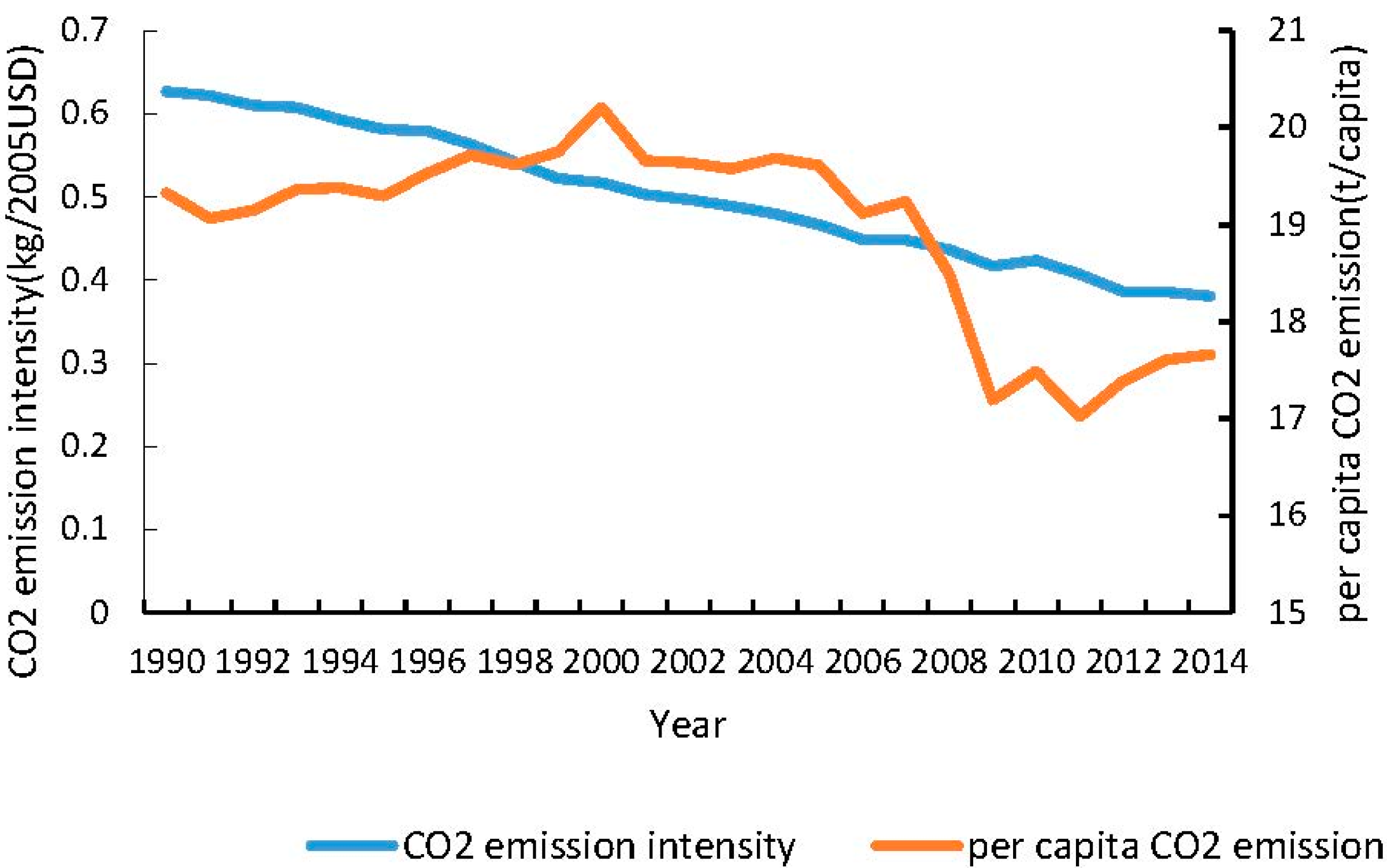
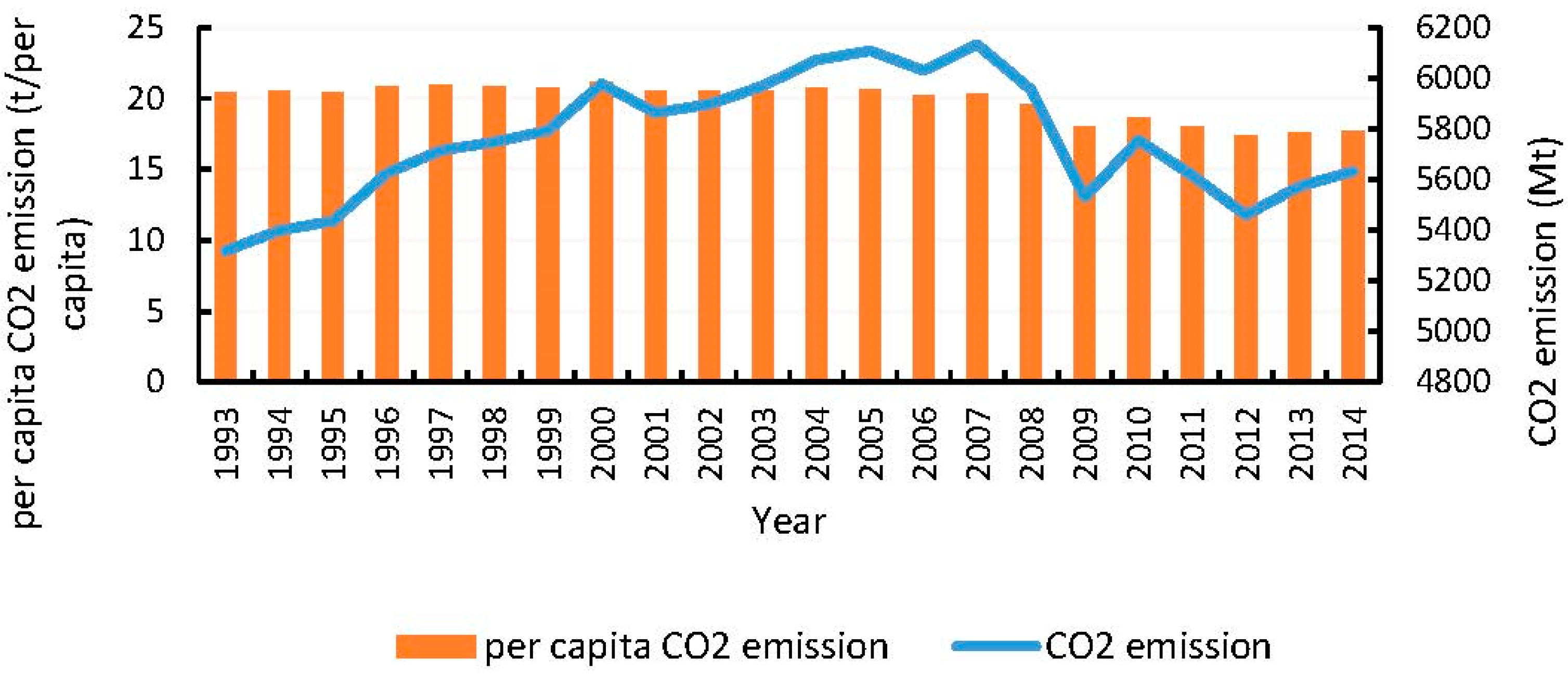
In the first stage (1990–2005), CO₂ emissions were on the rise, and the emission was 5795. 16 Mt in 2005 compared with 5161.03 Mt in 2005. However, in stage two (2006–2014), carbon dioxide emissions decreased to 5631.22 Mt in 2014. Per capita CO₂ emissions increased in the first stage while in stage 2 the figure started to fall. In general, per capita CO₂ emissions decreases by 14.58% from 1990 to 2014, and CO₂ emissions intensity has been dropping during the study period.

(2)

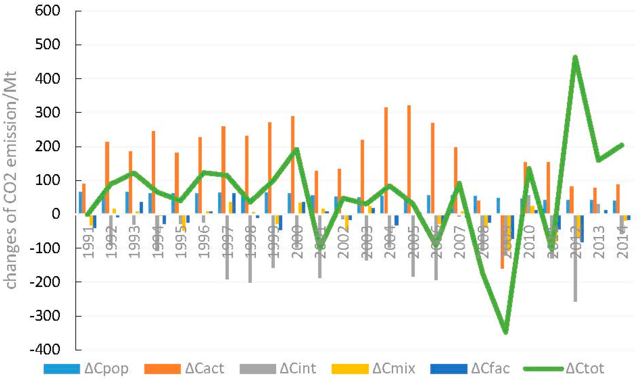
From the addictive decomposition of CO₂ emissions, we can arrive at some conclusions: economic activities effect was the chief factor of increasing the carbon dioxide emissions and energy intensity effect had significant impact on curbing the increase, in other words, it contributed to decreasing the carbon emissions. On the whole, population effect played a positive role in increasing CO₂ emissions and emission factor had a negative influence on it. Besides, energy mix effect had only a modest impact.

(3)

As indicated by the decoupling elasticity value from different effects, economic activities effect is the most significant among the five factors. When it comes to the decoupling effort index “relative decoupling” and “no decoupling” were the most common states. During stage 1, there were three years in the state of no decoupling which was caused by a short recession, nevertheless, the rest was “relative decoupling”. However, in the second phase, 5 years appeared to be in a “no decoupling” state, the rest mainly came with a state of “strong decoupling”, referring to an efficient and healthy way of economic growth.

5.2. Policy Implications

Emission reduction targets for the United States was to reduce greenhouse gas emissions by 28% by 2025, compared with 2005. Based on the actual situation, effective measures and policies should be taken to achieve this objective. At this point, some recommendations are put forward:

The economic activity effect was inextricably bound up with economy, there is no doubt that sound economic development constructs a major factor in restrict the exhaust of greenhouse gas. Moreover, developing low-carbon economy and adjusting industry structure are also sensible choices. In addition, educational programs make a positive impact on the decrease of carbon dioxide emissions. It is true that those earning master’s, doctoral, or professional degrees still earn more during their careers than those with less education. According to a report published by the Georgetown University Center for Education and the Workforce [65], those holding bachelor’s degrees earn about $2.27 million over their lifetime, while those with master’s, doctoral, and professional degrees earn $2.67 million, $3.25 million, and $3.65 million, respectively. As a result, the advancement of education level can make a contribution to the decrease of CO₂ emissions. As a result, the advancement of education level can make a contribution to the decrease of CO₂ emissions and the promotion of the relationship between economic activities and environmental changes.

Furthermore, energy intensity effect should be treated as a key issue. As stated above, energy intensity effect contributed to reducing CO₂ emissions. Research on improving the using efficiency of energy should be encouraged.

Though energy mix effect did not seem to be a key element that influenced carbon emissions, upgrading energy mix can be a beneficial way to limiting the growth of CO₂ and diminishing the harm on environment. Fossil fuel still provided the majority of energy consumption, which constricted the diminution of CO₂ emissions. In that case, it is urgent to optimize the energy mix. Generally speaking, reduction opportunities for CO₂ emissions were fulfilled in some aspects as follows: energy efficiency, energy conservation, fuel switching, and carbon capture and sequestration. Specifically, reducing personal energy use by turning off lights and electronics when not in use, the use of more efficient electrical appliances, using more renewable sources and fuels with lower carbon contents, improvement of CO₂ capture and sequestration technology in power plants and industrial processes are all ways to reduce carbon emissions. In particular, main policies and projects of America on energy efficiency are listed in

Table 7. Key energy-efficiency policies and programs.

Energy Policies	Date Effective
ENERGY STAR Program	1992
The Tax Incentives Assistance Project (TIAP)	2005
Revised Tax for investments in energy efficient commercial building	2005
Promoted research on GHG capture and storage options	2007
New efficiency standards for external power supplies	2007
New efficiency standards for in-home appliances	2007
New efficiency standards for electric motors	2007
Economy, Energy and Environment Program (E3)	2009
Energy efficiency upgrades in private and federal building	2009
$4.5 billion to increase energy efficiency in federal buildings (GSA)	2009
Greenhouse gas emissions new standards for cars and light trucks	2010
Tax credits for energy efficiency upgrades to existing homes purchased	2011
Incandescent light bulbs were slated to be phased out	2012
More funding for clean energy technology and efficiency improvement	2013
Builder incentives for energy efficient new homes	2014

[66,67,68,69,70,71,72,73,74,75].

Emission coefficient effect also played an important role in influencing carbon dioxide emissions. High-carbon energy mode should be transformed by low-carbon energy, for example, coal can be displaced by natural solar and nuclear power.

Although greenhouse gases have got people’s attention, people do not have enough attention to the specific factors that cause carbon emissions. To achieve the low carbon target, how to make people pay enough attention to curbing carbon dioxide emissions is the very issue the government should rethink.

References

1. Al-Mulali, U.; Fereidouni, H.G.; Lee, J.Y.M.; Che, N.B.C.S. Exploring the relationship between urbanization, energy consumption, and CO2 emission in MENA countries. Renew. Sustain. Energy Rev. 2013, 23, 107–112. [Google Scholar] [CrossRef]
2. Zhang, Y.J.; Da, Y.B. The decomposition of energy-related carbon emission and its decoupling with economic growth in China. Renew. Sustain. Energy Rev. 2015, 41, 1255–1266. [Google Scholar] [CrossRef]
3. Vavrek, R.; Chovancova, J. Decoupling of Greenhouse Gas Emissions from Economic Growth in V4 Countries. Procedia Econ. Financ. 2016, 39, 526–533. [Google Scholar] [CrossRef]
4. Dong, J.F.; Wang, Q.; Deng, C.; Wang, X.M.; Zhang, X.L. How to Move China toward a Green-Energy Economy: From a Sector Perspective. Sustainability 2016, 8, 337. [Google Scholar] [CrossRef]
5. Wang, Q.; Chen, Y. Energy saving and emission reduction revolutionizing China’s environmental protection. Renew. Sustain. Energy Rev. 2009, 14, 535–539. [Google Scholar] [CrossRef]
6. Komal, R.; Abbas, F.; Komal, R.; Abbas, F. Linking financial development, economic growth and energy consumption in Pakistan. Renew. Sustain. Energy Rev. 2015, 44, 211–220. [Google Scholar] [CrossRef]
7. Grand, M.C. Carbon emission targets and decoupling indicators. Ecol. Indic. 2016, 67, 649–656. [Google Scholar] [CrossRef]
8. Global Carbon-Dioxide Emissions Increase by 1.0 Gt in 2011 to Record High. Available online: http://www.iea.org/newsroOmandevents/news/2012/may/global-carbon-dioxide-emissions-increase-by-10-gt-in-2011-to-record-high.html (accessed on 24 May 2012).
9. Steckel, J.C.; Jakob, M.; Marschinski, R.; Luderer, G. From carbonization to decarbonization—Past trends and future scenarios for China’s CO2 emissions. Energy Policy 2011, 39, 3443–3455. [Google Scholar] [CrossRef]
10. Stelling, P. Policy instruments for reducing CO2 emissions from the Swedish freight transport sector. Res. Trans. Bus. Manag. 2014, 12, 47–54. [Google Scholar] [CrossRef]
11. Francey, R.J.; Trudinger, C.M.; Schoot, M.V.D.; Law, R.M.; Krummel, P.B.; Langenfelds, R.L.; Steele, L.P.; Allison, C.E.; Stavert, A.R.; Andres, R.J.; et al. Atmospheric verification of anthropogenic CO2 emission trends. Nat. Clim. Chang. 2013, 3, 520–524. [Google Scholar] [CrossRef]
12. Wang, Q. Cheaper oil challenge and opportunity for climate change. Environ. Sci. Technol. 2015, 49, 1997–1998. [Google Scholar] [CrossRef] [PubMed]
13. Wang, Q. Effective policies for renewable energy—The example of China’s wind power—Lessons for China’s photovoltaic power. Renew. Sustain. Energy Rev. 2010, 14, 702–712. [Google Scholar] [CrossRef]
14. Wang, Q.; Chen, X. Rethinking and reshaping the climate policy: Literature review and proposed guidelines. Renew. Sustain. Energy Rev. 2013, 21, 469–477. [Google Scholar] [CrossRef]
15. Baldwin, J.G.; Wing, I.S. The spatiotemporal evolution of U.S. carbon dioxide emissions: Stylized facts and implications for climate policy. Reg. Sci. 2013, 53, 672–689. [Google Scholar] [CrossRef]
16. Shahbaz, M.; Khraief, N.; Jemaa, M.M.B. On the causal nexus of road transport CO2 emissions and macroeconomic variables in Tunisia: Evidence from combined cointegration tests. Renew. Sustain. Energy Rev. 2015, 51, 89–100. [Google Scholar] [CrossRef]
17. Wang, Q. China’s citizens must act to save their environment. Nature 2013, 497, 159–159. [Google Scholar] [CrossRef] [PubMed]
18. Jain, N.; Arora, P.; Tomer, R.; Mishra, S.V.; Bhatia, A.; Pathak, H.; Chakraborty, D.; Kumar, V.; Dubey, D.S.; Harit, R.C.; et al. Greenhouse gases emission from soils under major crops in northwest India. Sci. Total Environ. 2016, 542, 551–561. [Google Scholar] [CrossRef] [PubMed]
19. Timilsina, G.R.; Shrestha, A. Transport sector CO2 emissions growth in Asia: Underlying factors and policy options. Energy Policy 2009, 37, 4523–4539. [Google Scholar] [CrossRef]
20. Wang, Q. China should aim for a total cap on emissions. Nature 2014, 512, 115. [Google Scholar] [CrossRef] [PubMed]
21. Wang, Q.; Li, R.R. Cheaper Oil: A turning point in Paris climate talk? Renew. Sustain. Energy Rev. 2015, 52, 1186–1192. [Google Scholar] [CrossRef]
22. Wang, Z.H.; Yang, L. Delinking indicators on regional industry development and carbon emissions: Beijing–Tianjin–Hebei economic band case. Ecol. Indic. 2015, 48, 41–48. [Google Scholar] [CrossRef]
23. Wang, Q. China has the capacity to lead in carbon trading. Nature 2013, 493, 273. [Google Scholar] [CrossRef] [PubMed]
24. Wang, Q.; Chen, X. Energy policies for managing China’s carbon emission. Renew. Sustain. Energy Rev. 2015, 50, 470–479. [Google Scholar] [CrossRef]
25. Štreimikienė, D. Residential energy consumption trends, main drivers and policies in Lithuania. Renew. Sustain. Energy Rev. 2014, 35, 285–293. [Google Scholar] [CrossRef]
26. Guan, D.; Peters, G.P.; Weber, C.L.; Hubacek, K. Journey to world top emitter: An analysis of the driving forces of China’s recent CO2 emissions surge. Geophys. Res. Lett. 2009. [Google Scholar] [CrossRef]
27. Wang, Q.; Li, R.R. Journey to burning half of global coal: Trajectory and drivers of China’s coal use. Renew. Sustain. Energy Rev. 2016, 58, 341–346. [Google Scholar] [CrossRef]
28. Wang, Q.; Chen, Y. Status and outlook of China’s free-carbon electricity. Renew. Sustain. Energy Rev. 2010, 14, 1014–1025. [Google Scholar] [CrossRef]
29. Yu, S.W.; Zhang, J.J.; Zheng, S.H.; Sun, H. Provincial carbon intensity abatement potential estimation in China: A PSO-GA-optimized multi-factor environmental learning curve method. Energy Policy 2015, 77, 46–55. [Google Scholar] [CrossRef]
30. Wang, Q.; Chen, X. China’s electricity market-oriented reform: From an absolute to a relative monopoly. Energy Policy 2012, 51, 143–148. [Google Scholar] [CrossRef]
31. Xu, B.; Lin, B.Q. How industrialization and urbanization process impacts on CO2 emissions in China: Evidence from nonparametric additive regression models. Energy Econ. 2015, 48, 188–202. [Google Scholar] [CrossRef]
32. Wang, Q.; Li, R. Impact of cheaper oil on economic system and climate change: A SWOT analysis. Renew. Sustain. Energy Rev. 2016, 54, 925–931. [Google Scholar] [CrossRef]
33. Aydin, G. The Development and Validation of Regression Models to Predict Energy-related CO2 Emissions in Turkey. Energy Sources Part B 2015, 10, 176–182. [Google Scholar] [CrossRef]
34. Wang, Q.; Chen, X.; Jha, A.N.; Rogers, H. Natural gas from shale formation—The evolution, evidences and challenges of shale gas revolution in United States. Renew. Sustain. Energy Rev. 2014, 30, 1–28. [Google Scholar] [CrossRef]
35. Wang, Q.; Li, R. Natural gas from shale formation: A research profile. Renew. Sustain. Energy Rev. 2016, 57, 1–6. [Google Scholar] [CrossRef]
36. Wang, Q.; Li, R. Drivers for energy consumption: A comparative analysis of China and India. Renew. Sustain. Energy Rev. 2016, 62, 954–962. [Google Scholar] [CrossRef]
37. Wang, Q.; Li, R. Sino-Venezuelan oil-for-loan deal—The Chinese strategic gamble? Renew. Sustain. Energy Rev. 2016, 64, 817–822. [Google Scholar] [CrossRef]
38. Andreoni, V.; Galmarini, S. Decoupling economic growth from carbon dioxide emissions: A decomposition analysis of Italian energy consumption. Energy 2012, 44, 682–691. [Google Scholar] [CrossRef]
39. Cansino, J.M.; Sánchez-Braza, A.; Rodríguez-Arévalo, M.L. Driving forces of Spain’s CO2 emissions: A LMDI decomposition approach. Renew. Sustain. Energy Rev. 2015, 48, 749–759. [Google Scholar] [CrossRef]
40. Hasanbeigi, A.; Price, L.; Fino-Chen, C.; Lu, H.; Ke, J. Retrospective and prospective decomposition analysis of Chinese manufacturing energy use and policy implications. Energy Policy 2013, 63, 562–574. [Google Scholar] [CrossRef]
41. Xie, S.C. The driving forces of China’s energy use from 1992 to 2010: An empirical study of input-output and structural decomposition analysis. Energy Policy 2014, 73, 401–415. [Google Scholar] [CrossRef]
42. Valeria, A.; Stefano, G. Drivers in CO2 emissions variation: A decomposition analysis for 33 world countries. Energy 2016, 103, 27–37. [Google Scholar]
43. Inglesi-Lotz, R.; Pouris, A. Energy efficiency in South Africa: A decomposition exercise. Energy 2012, 42, 113–120. [Google Scholar] [CrossRef]
44. Tunç, G.I.; Türüt-Aşık, S.; Akbostanci, E. A decomposition analysis of CO2 emissions from energy use: Turkish case. Energy Policy 2009, 37, 4689–4699. [Google Scholar] [CrossRef]
45. Ozturk, I.; Acaravci, A. CO2 emissions, energy consumption and economic growth in Turkey. Renew. Sustain. Energy Rev. 2010, 14, 3220–3225. [Google Scholar] [CrossRef]
46. Diakoulaki, D.; Mandaraka, M. Decomposition analysis for assessing the progress in decoupling industrial growth from CO2 emissions in the EU manufacturing sector. Energy Econ. 2007, 29, 636–64. [Google Scholar] [CrossRef]
47. González, P.F.; Moreno, B. Analyzing driving forces behind changes in energy vulnerability of Spanish electricity generation through a Divisia index-based method. Energy Convers. Manag. 2015, 92, 459–468. [Google Scholar] [CrossRef]
48. Ang, B.W.; Liu, F.L.; Chew, E.P. Perfect decomposition techniques in energy and environmental analysis. Energy Policy. 2003, 31, 1561–1566. [Google Scholar] [CrossRef]
49. Ang, B.W. Decomposition analysis for policymaking in energy: Which is the preferred method? Energy Policy 2004, 32, 1131–1139. [Google Scholar] [CrossRef]
50. Schandl, H.; Hatfield-Dodds, S. Decoupling global environmental pressure and economic growth: Scenarios for energy use, materials use and carbon emissions. J. Clean. Prod. 2016, 132, 45–56. [Google Scholar] [CrossRef]
51. Wang, Q.W.; Hang, Y. Decoupling and attribution analysis of industrial carbon emissions in Taiwan. Energy 2016, 113, 728–738. [Google Scholar] [CrossRef]
52. Dong, J.F.; Deng, C.; Wang, X.M.; Zhang, X.L. Multilevel Index Decomposition of Energy-Related Carbon Emissions and Their Decoupling from Economic Growth in Northwest China. Energies 2016, 9, 680. [Google Scholar] [CrossRef]
53. Tapio, P. Towards a theory of decoupling: Degrees of decoupling in the EU and the case of road traffic in Finland between 1970 and 2001. Transp. Policy 2005, 12, 137–151. [Google Scholar] [CrossRef]
54. Kaya, Y.; Yokoburi, K. Environment, Energy, and Economy: Strategies for Sustainability, 1st ed.; United Nations University Press: Tokyo, Japan, 1997; pp. 16–26. [Google Scholar]
55. Wang, Q.; Chen, Y. Barriers and opportunities of using the clean development mechanism to advance renewable energy development in China. Renew. Sustain. Energy Rev. 2010, 14, 1989–1998. [Google Scholar] [CrossRef]
56. Ang, B.W. The LMDI approach to decomposition analysis: A practical guide. Energy Policy 2005, 33, 867–871. [Google Scholar] [CrossRef]
57. Ang, B.W. LMDI decomposition approach: A guide for implementation. Energy Policy 2015, 86, 233–238. [Google Scholar] [CrossRef]
58. Zhao, M.; Tan, L.R.; Zhang, W.G.; Ji, M.H.; Liu, Y.; Yu, L.Z. Decomposing the influencing factors of industrial carbon emissions in Shanghai using the LMDI method. Energy 2010, 35, 2505–2510. [Google Scholar] [CrossRef]
59. Wang, W.W.; Zhang, M.; Zhou, M. Using LMDI method to analyze transport sector CO2 emissions in China. Energy 2011, 36, 5909–5915. [Google Scholar] [CrossRef]
60. Vehmas, J.; LuUKkanen, J.; Kaivo-oja, J. Linking analyses and environmental Kuznets curves for material flows in the European Union 1980–2000. J. Clean. Prod. 2007, 15, 1662–1673. [Google Scholar] [CrossRef]
61. The World Bank. Available online: http://www.worldbank.org/html (accessed on 25 July 2016).
62. BP Statistical Review of World Energy. Available online: http://www.bp.com/en/global/corporateenergy-economics/statistical-review-of-world-energy.html (accessed on 25 July 2016).
63. Consumption-Based Accounting of CO2 Emissions. Available online: http://www.pnas.org/content/107/12/5687 (accessed on 25 July 2016).
64. The China-US Climate Change Agreement Is a Step forward for Green Power Relations. Available online: https://www.theguardian.com/commentisfree/2014/nov/14/the-china-us-climate-change-agreement-is-a-step-forward-for-green-power-relations (accessed on 25 July 2016).
65. How Higher Education Affects Lifetime Salary. Available online: http://www.usnews.com/education/best-colleges/articles/2011/08/05/how-higher-education-affects-lifetime-salary (accessed on 25 July 2016).
66. The Simple Choice for Energy Efficiency-Energy Star. Available online: https://www.energystar.gov/ (accessed on 25 July 2016).
67. The Tax Incentives Assistance Project (TIAP). Available online: http://www.energytaxincentives.org/ (accessed on 25 July 2016).
68. Energy Policy Act of 2005 (Energy Bill). Available online: http://www.lse.ac.UK/GranthamInstitute/law/energy-policy-act-2005-energy-bill/ (accessed on 25 July 2016).
69. Renewable Fuels, Consumer Protection, and Energy Efficiency Act of 2007 110th Congress (2007–2008). Available online: https://www.congress.gov/bill/110th-congress/senate-bill/1419 (accessed on 25 July 2016).
70. E3: Economy-Energy-Environment. Available online: https://www.epa.gov/e3 (accessed on 25 July 2016).
71. American Recovery and Reinvestment Act of 2009. Available online: http://www.va.gov/recovery/ (accessed on 25 July 2016).
72. American Power Act of 2010. Available online: http://aceee.org/topics/american-power-act-2010 (accessed on 25 July 2016).
73. Clean Energy Regulator Act 2011 No. 163. 2011. Available online: https://www.legislation.gov.au/Details/C2011A00163 (accessed on 25 July 2016).
74. Climate Action Plan of 2013. Available online: https://www.whitehouse.gov/the-press-office/2013/06/25/fact-sheet-president-obama-s-climate-action-plan (accessed on 25 July 2016).
75. Fact Sheet: 2014 U.S. CLimate Action Report. Available online: http://www.state.gov/e/oes/rls/rpts/car6/219259.htm (accessed on 25 July 2016).
Figure 1. Change rates of per capita CO2 emissions and CO2 emission intensity in America during 1990–2014 (1990 as the baseline year).
Sustainability 08 00857 g001
Figure 2. The changes of CO2 emissions and per capita CO2 emission in America.
Sustainability 08 00857 g002
Figure 3. Decomposition of changes of CO2 emissions in America.
Sustainability 08 00857 g003