Effects of Water Management Strategies on Water Balance in a Water Scarce Region: A Case Study in Beijing by a Holistic Model

Abstract

Irrigation is facing increasing pressure from other competitive water users to reduce water consumption in a water scarce region. Based on the Basin-wide Holistic Integrated Water Assessment (BHIWA) model, the effects of water management strategies on water balance in the dry regions of North China were analyzed. The results show that, with the decrease of irrigation water supply reliability (IWSR) and the increase of irrigation water use efficiency (WUE), irrigation water use decreased significantly, leading to reduced agriculture water consumption, and sustained ground water levels. Compared with the increase of WUE, the decrease of IWSR contributes more to reducing irrigation water consumption and protecting groundwater. Sensitivity tests show that among various water cycle components, irrigation water use is most sensitive to changes, followed by agriculture water consumption, and then groundwater level. Reducing IWSR is an effective strategy to reduce irrigation water consumption and promote sustainable water resources management, which could be the support of basic data and theory for regional water resources planning.

1. Introduction

With the acceleration of urbanization, the problem of water shortage is becoming more and more serious around large urban centers [1,2,3]. To cope with the increasing pressure on water resources, China adopted a pro-active approach to building a “water-saving society” which focuses on water-saving in society and especially in agriculture, which is the biggest user of water. Improving water use efficiency (WUE) in agriculture helps reduce irrigation water losses through seepage, percolation, and runoff. However, in areas where water scarcity is due to structural shortage in the availability of water, demand management becomes necessary to constrain agricultural water consumption, and reallocate water to other competitive users, or even allow for provisions of environmental water requirements such as groundwater conservation by avoiding over-exploitation [4,5,6,7,8].

Beijing is one of the most water-stressed large cities in the world, where the annual internally renewable water resource per capita is about 100 m³ [9,10,11]. The lack of water has led to degradation of the natural ecosystem in the city, and the operation of the resources and the environment being overloaded, which has seriously restricted the sustainable development of Beijing [12,13]. To cope with water scarcity, the total amount of water consumed by agriculture has been reduced with measures such as the adjustment of crop planting structure and the adoption of high-efficiency water-saving technologies in agriculture. Consequently, the proportion of agricultural water use to total water use decreased from 45% in 2001 to 22% in 2014, while the WUE increased from 0.55 in 2001 to about 0.70 at present [9,14]. However, the groundwater table in Beijing continues to decline in recent years, which poses a serious threat to the environment. Therefore, further reduction in agricultural water use is needed. The question is how the further reduction could be achieved with minimal negative impacts on agriculture. There is a need to quantify the effects of different water saving irrigation practices on regional hydrological cycle components, from which more effective interventions could be identified and promoted.

Hydrological models are widely used to research water management issues, by increasing the systematic observable, eliminating the interference factors, and pining the actual relations among variables of the basin water cycles [15,16,17]. The Basin-wide Holistic Integrated Water Assessment (BHIWA) model developed by the International Committee of Irrigation Drainage (ICID) features concise calculation, clear concept, easily accessible data, and the ability to simulate the whole process of the water cycle. The model is especially suitable for the simulation of the influence on the regional water cycle process from the changes of agricultural irrigation strategies, and has been applied successfully in the researches on many basin hydrological cycles of India and China [18,19,20,21]. The BHIWA model was selected as the regional water balance analysis tool in Beijing Daxing County, and the regional water resources consumption, the regional water withdrawals, and the water situation indicators were analyzed. Analysis showed that to assure the sustainable utilization of water resources, effective water resources management measures should have to be put into use such as high water use efficiency, good crop structure, water resources importation, and so on [22].

The objective of this paper is to assess potential interventions in reducing irrigation water supply and uses, and identify strategies for effectively reducing agricultural water consumption in the highly water scarce Beijing Metropolitan. Section 2 of the paper gives a brief introduction to the study area, followed with an introduction to the BIHWA model and model evaluation indexes. Section 3 presents the outputs of the model simulations based on several water-saving and management scenarios; the one at a time (OAT) approach for sensitivity analysis is adopted to identify key practices leading to expected outcomes of maximum water consumption at the regional level. Finally, we concluded the paper with recommendations for alternate irrigation water management strategies to reduce agricultural water consumption in water scarce peri-urban agricultural systems.

2. Materials and Methods

2.1. Study Area

Beijing, located in the North China Plain, is one of the most rapid transforming mega-cities in the world. With a population of about 20 million, the city is under extreme pressure to manage its land and water resources. Agriculture in the metropolitan area has decreased from 3.439 × 10⁵ hm⁻² in year 1996 to 2.212 × 105 hm⁻² in year 2013 [23,24]. Daxing County is an administrative unit of the city with relatively large agricultural areas, between latitude of 39°26′ and 39°50′ N, and longitude of 116°13′ and 116°43′ E. The agricultural water use in Daxing was 0.22 billion cubic meters, about 27% of Beijing agricultural water use, in 2014 [9]. Daxing has a warm and continental monsoon climate. The mean annual temperature is 12 °C [25]. The mean annual evaporation is 1800 mm and the mean annual precipitation is 472 mm, about 400 mm of which falls in the summer months from June to September. There is a decreasing trend in annual precipitation starting from 1970s, while dry years were also observed in 1980–1994 and 1999–2005 [25]. There are four rivers in the Daxing County. The rivers are usually dry except the Liangshui River and the Xinfeng River, which carries passing-by sewage water. The local water supply is mainly from groundwater. With the increase of water use, the groundwater level in general has been decreasing since 1980s. The depth of groundwater was 3.1 m in 1980, but the depth of groundwater was 14.7 m in 2003 [25]. So, the over-exploitation of groundwater was serious for Daxing County. In a word, the proportion of agricultural water use is larger, and the situation of water shortage is serious. For sustainable utilization of water resources in Daxing County, effective management measures should be adopted in the future. In this paper, the whole Daxing County was selected as the study area.

2.2. The BHIWA Model Description

The BHIWA hydrological model is capable of simulating the hydrological effects of irrigation development and land-use changes [26]. The BHIWA model has several components including those on surface water balance, groundwater balance, their interactions, as well as the effects of irrigation water withdrawal on water storages and water consumption. The modeling parameters include landuse, soil hydraulic properties, water resources interactions, etc.

2.2.1. Irrigation Water Use

The source of irrigation is mainly groundwater in the Daxing County. The amount of extraction is estimated using below equation:

$$W{D}_{GW IR}=(E{T}_I+DP)/WU{E}_{GW}$$

(1)

where WD_{GW IR} is the groundwater withdrawal required for irrigation, ET_I is the evapotranspiration from irrigation, DP is the deep percolation for paddy, and WUE_GW is the water use efficiency of groundwater irrigation.

2.2.2. Agriculture Water Use Consumption

The agriculture water consumption for the irrigation systems is divided into precipitation evapotranspiration, irrigation evapotranspiration, and irrigation water logged evapotranspiration. The precipitation evapotranspiration is restricted to the precipitation quantity and the planting structure of underlying surface. The irrigation evapotranspiration is caused by irrigation. The calculation formula for agriculture water consumption is as follows:

$$E{T}_a\equiv E{T}_P+E{T}_I+E{T}_{Swamps}$$

(2)

where ET_a is the evapotranspiration from agriculture, ET_P is the evapotranspiration for precipitation, and ET_Swamps is the evapotranspiration from irrigation water logged areas.

2.2.3. Groundwater Level

Based on water quantity balance of groundwater system, the groundwater level variation is caused by net groundwater exploitation. The calculation formula for groundwater level is as follows:

$$H=H_0+\frac{NGU}{\mu A}$$

(3)

where H₀ is the average groundwater level in the current year, NGU is the net groundwater exploitation, µ is the regional synthetic specific yield of groundwater storage variation, and A is the study area.

2.3. Scenarios

Two types of interventions were considered for effectively reducing irrigation water use. The first one tries to examine the effects of reduced irrigation water supply reliability (IWSR) on total water use. The second one uses WUE to represent engineering and management efficiency measures such as canal lining, water saving irrigation, and irrigation scheduling. By changing the target thresholds of these two indicators, we simulated the responses of irrigation systems and assessed the changes in water balance components using the BHIMA model.

The above interventions were simulated for a set of climate conditions being wet, normal, dry, and extremely dry years. The precipitation data of 1976–2005 were selected for frequency analysis in Daxing County. The P-III distribution curve was selected as the theoretic frequency curve, where the variation and deviation coefficient estimated were 0.31 and 1.09, respectively; the points of little or moderate precipitation were fitting well, and the annual precipitation data with different frequencies were obtained and are shown in

Table 1. Selected typical wet, normal, dry, and extremely dry years and their frequency distribution.

Precipitation Type	Wet	Normal	Dry	Extremely Dry	Average
Frequency (%)	25	50	75	90	-
Annual precipitation (mm)	551	446	365	310	472

.

Sensitivity analysis is used to investigate how variation in model outputs can be apportioned to variation in its inputs. The most common approach for sensitivity analysis is changing one model input at a time to see how this input parameter affects the model output (OAT) [27,28,29,30]. The relative sensitivity was used for the evaluation of sensitivity of irrigation supply, agriculture water consumption, and regional groundwater level. Relative sensitivity was calculated based on the OAT approach in this study. The equation for relative sensitivity (RD) follows [31]:

$$RD=\frac{\left|Y_{i+1}-Y_i\right|}{\left|X_{i+1}-X_i\right|}\times \frac{X_i}{Y_i}$$

(4)

where X_i+1 and X_i are the index values under I + 1 and i level respectively, Y_i+1 and Y_i are the response variables simulated with BHIWA model under I + 1 and i level of the index values respectively. The greater the relative sensitivity value, the stronger relation the parameters and outputs are associated. The value of index level selection is shown in

Table 2. The range and intevals of parameter value inputs for sensitivity analysis.

Index	Index Range	Value of Index Level Selection
Irrigation water supply reliability (IWSR)	0.0~1.0	0.0, 0.1, 0.2, 0.3, 0.4, 0.5, 0.6, 0.7, 0.8, 0.9, 1.0
Irrigation water use efficiency (WUE)	0.60~0.90	0.60, 0.65, 0.70, 0.75, 0.80, 0.85, 0.90

.

2.4. Evapotranspiration (ET) Data for the BHIWA Model

Research has pointed out limitations in validating hydrological models using river flow data. Validation of regional hydrological model are affected by the representativeness of the gauge stations and the uncertainty of the hydrologic processes [32,33,34]. In this paper, remote sensing based ET maps were used to validate the BHIWA model.

The ET maps were produced by Wu et al. (2012), using the ETWatch model from 2004 to 2005 at a spatial and temporal resolution of 30 meters and 15 days, respectively.

The maps were validated with field measurements at the study area with accuracy of 90% in the agricultural area [35]. Details about the ETWatch model are reported by Wu et al. (2008, 2010) [36,37].

The BHIWA model was calibrated and validated based on input data such as land use data, monitoring hydrological and meteorological data, crop parameter data, and so on between 2004 and 2005. The ET from different land use in BHIWA was calibrated using the RS ET in 2004, and further validated using the 2005 RS ET.

2.5. Simulated Evaluation Indexes

The performance of the model was evaluated using the root mean square error (RMSE), the mean absolute error (MAE), and the mean bias error (MBE), all of which can be expressed in units of the ET and the Willmott index of agreement [38,39,40].

The RMSE gives the weighted variations in errors (residual) between the modeled and remote sensing ET (RS ET) values and was calculated as follows:

$$RMSE=\sqrt{\frac{1}{n}{\displaystyle {\sum }_{i=1}^n{\left(M_i-O_i\right)}^2}}$$

(5)

where n is the number of the land use, $M_i$ is the modeled ET, and $O_i$ is the remote sensing evapotranspiration (RS ET). The mean absolute error (MAE) measures the weighted average magnitude of the absolute errors and was calculated as follows:

$$MAE=\frac{1}{n}{\displaystyle {\sum }_{i=1}^n\left|M_i-O_i\right|}$$

(6)

The MBE is an indicator of whether the model is under-predicting or over-predicting the RS ET value and also gives the uniformity of error distribution. Positive MBE values indicate over-prediction, negative values indicate under-prediction, and a value of zero indicates equal distribution between negative and positive values. The MBE was calculated as follows:

$$MBE=\frac{1}{n}\left[{\displaystyle {\sum }_{i=1}^n\left(M_i-O_i\right)}\right]$$

(7)

The Willmott index of agreement (d) is a descriptive measure and has values ranging from 0 to 1 [39]. The higher the index value the better the model performance. The d was calculated as follows:

$$d=1-\left[\frac{{\displaystyle {\sum }_{i=1}^n{\left(M_i-O_i\right)}^2}}{{\displaystyle {\sum }_{i=1}^n{\left(\left|M_i-\stackrel{-}{O}\right|+\left|O_i-\stackrel{-}{O}\right|\right)}^2}}\right]$$

(8)

where $\stackrel{-}{O}$ is the average value of RS ET for different land use; the other parameters have already been defined.

3. Results and Discussion

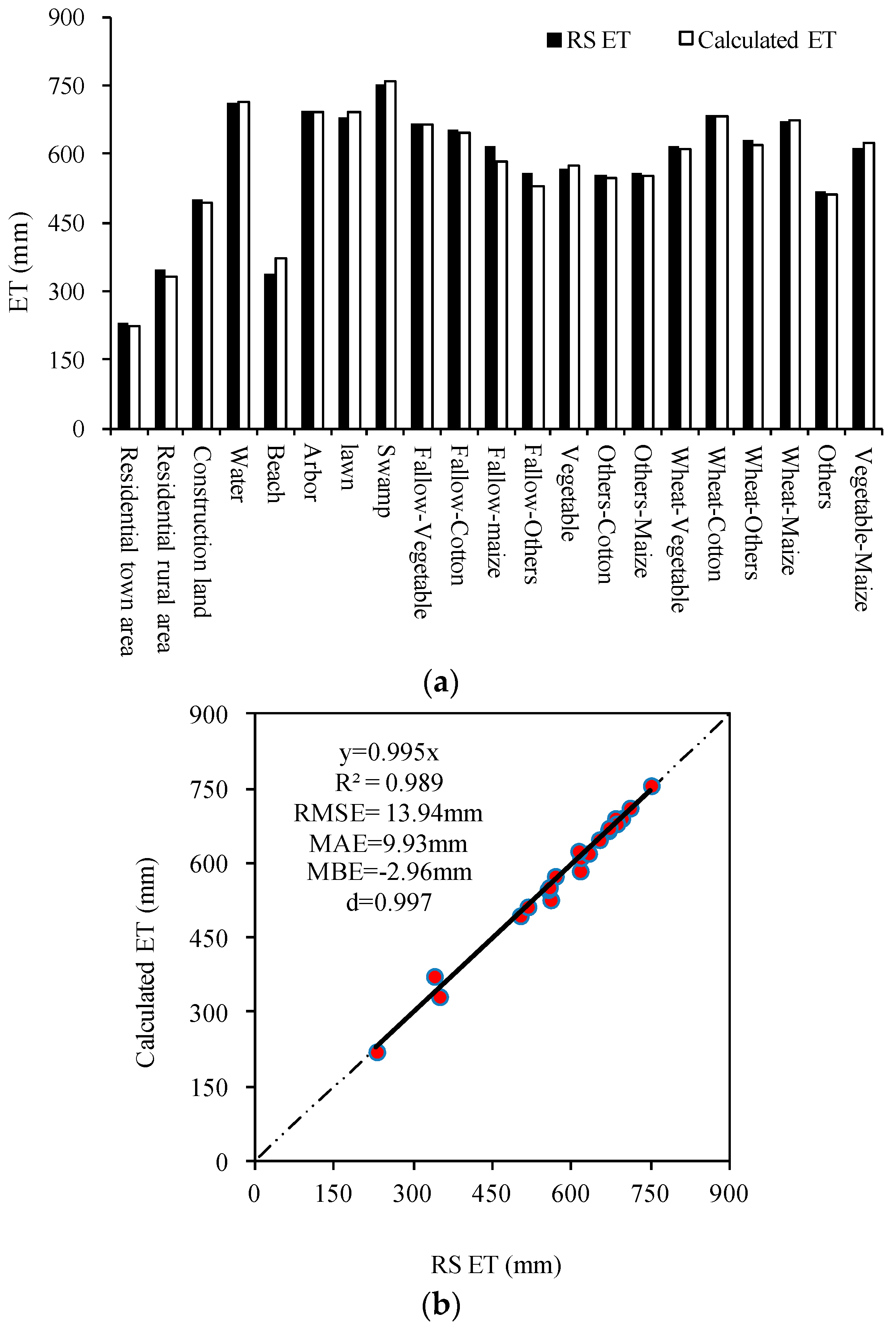
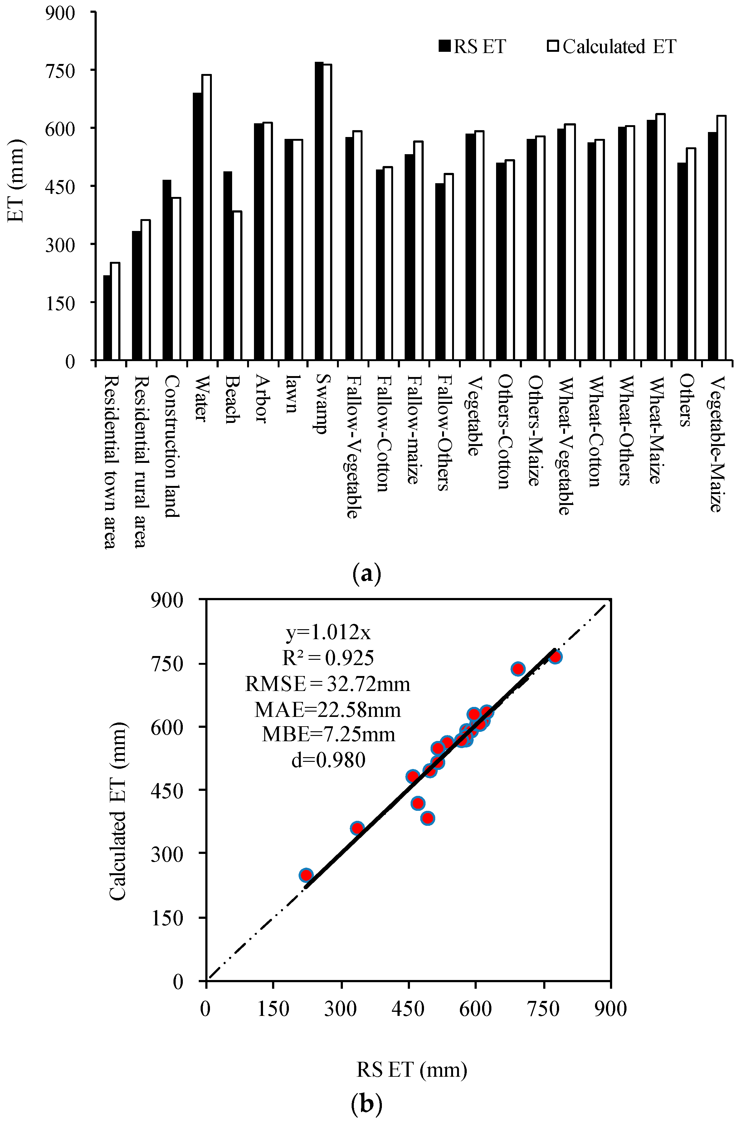
3.1. Calibration and Verification of BHIWA Model

Figure 1 shows the comparison of the calculated ET and RS ET for model calibration. In general, the calculated ET values follow closely the trend of the RS ET values for all the land use. On the other hand, Figure 1b shows the linear relationship between the RS ET and BHIWA modeled ET for all the land use. The RS ET and BHIWA modeled ET correlated well with an R² of 0.989 (p < 0.001). The BHIWA modeled ET was not significantly different from the RS ET values, with RMSE, MAE, and MBE values of 13.94, 9.93, and −2.96 mm, respectively. So, crop ET was simulated better. On the basis of this, the simulated precision was accepted. Based on the calibrated result, main parameters of the model were adopted as follows: (1) the soil moisture capacity was different for different land use such as arbor land (200 mm), winter wheat (100 mm), other agricultural areas (75 mm), residential areas (30 mm), and so on; (2) the reasonable outflow and groundwater recharge could be required based on the assumption of 40% residual water quantity towards surface runoff; (3) the exponential index linking soil moisture availability was 0.8; and (4) the recession coefficient for ground water reservoir was 0.25.

Figure 2 shows the comparison of the calculated ET and RS ET for model validation. At the same time, the BHIWA calculated ET values follow closely the trend of the RS ET values for all the land use. Figure 2b shows the linear relationship between the RS ET and BHIWA modeled ET for all the land use. The RS ET and BHIWA modeled ET correlated well with an R² of 0.925 (p < 0.001). The BHIWA modeled ET was not significantly different from the RS ET values with RMSE, MAE, and MBE values of 32.72, 22.58, and 7.25 mm, respectively. Overall, the results of model calibration and validation showed that the R² and d values between the RS ET values and BHIWA simulated ET values were much more than 0.92 and 0.98, respectively. Meantime, the RMSE, MAE, and MBE were less than 33, 23, and 7.3 mm, respectively. Consequently, the BHIWA model can be used to simulate the crop ET values with some degree of accuracy.

The results from model calibration and validation showed that the BHIWA could be used to simulate the crop ET values under different land use. Meanwhile, The BHIWA was used to simulate the groundwater storage variation with the Nash efficiency coefficient larger than 0.55 [37]. So, to simulate groundwater variation based on the BHIWA is credible. In this paper, effects of different irrigation water management strategies on water balance was studied based on vivificated BHIWA model, which should be conducive to irrigation water management for Beijing well region.

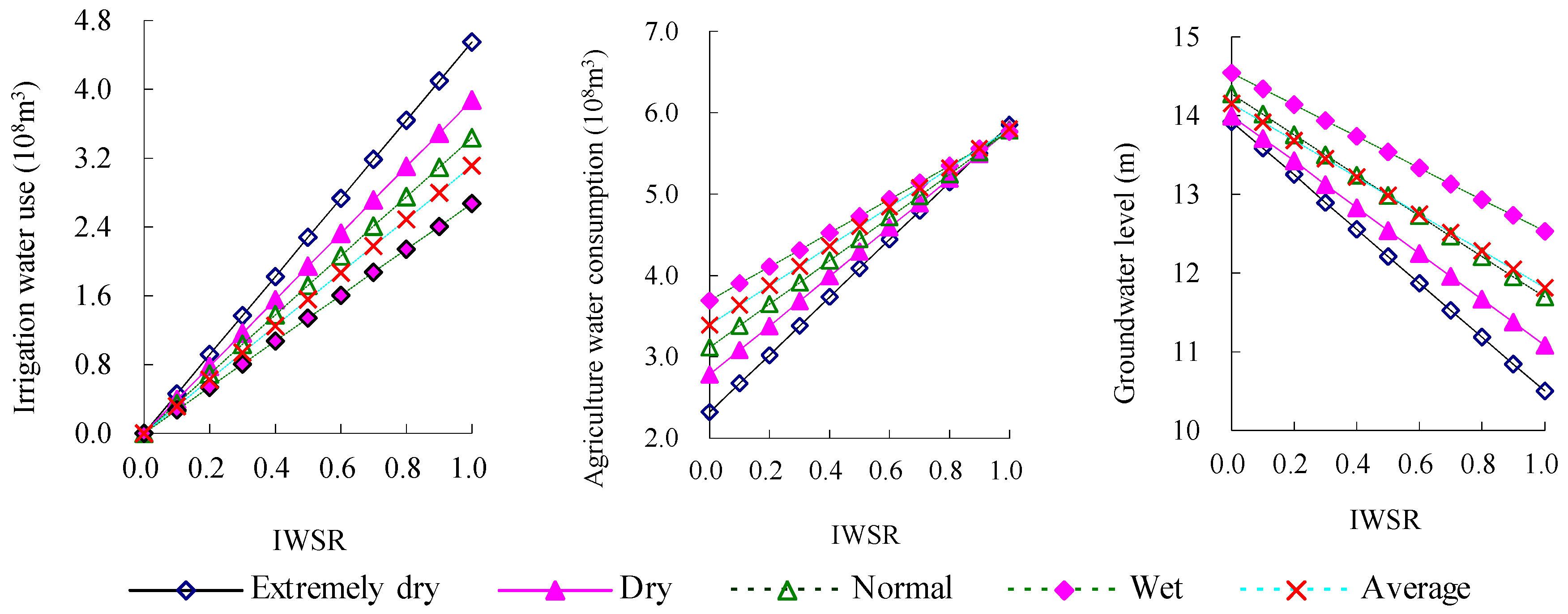
3.2. Effect of the Decrease of IWSR on Regional Irrigation Water Supply, Total Consumption, and Groundwater Level

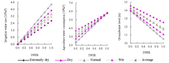
3.2.1. Variation of Regional Irrigation Water Use and Agriculture Water Consumption

The effect of the decrease of IWSR on the regional water supply and consumption is shown in Figure 3. With WUE set at 0.75, decreases in IWSR leads to significant decrease in irrigation water supply and total agricultural water consumption, and increased groundwater level. The variation of irrigation water supply, agriculture water consumption, and groundwater level with the increase of IWSR by 0.1 is shown in

Table 3. The variation of irrigation water use, agriculture water consumption and groundwater level with the increase by 0.1 of IWSR.

Precipitation Type	Extremely Dry	Dry	Normal	Wet	Average
Decrease of irrigation water use (108 m3)	0.455	0.388	0.344	0.267	0.311
Decrease of agriculture water consumption (108 m3)	0.353	0.301	0.267	0.208	0.241
Raise of groundwater level (m)	0.342	0.291	0.258	0.201	0.234

. Under different hydrological years, with the decrease of IWSR, water cycle components’ variation is different. With the decrease of IWSR, the water cycle components in dry years were affected much more than that in wet years. Compared with the wet year, with the decrease of IWSR by 0.1 in dry years, irrigation water use decreased by about 0.186 × 10⁸ m³, agriculture water consumption decreased by about 0.145 × 10⁸ m³, and the regional groundwater level raised to about 0.141 m. Crop water requirements are mainly from irrigation in dry years, which will result much more water withdrawal. Therefore, based on crop water production functions, the IWSR could be decreased properly by deficit irrigation in dry years. As a result, agriculture water consumption reduced greatly, and the groundwater was protected. Meanwhile, the crop yield was not seriously affected. In a word, there is a realistic significance for water resources shortage to promote a virtuous circle of the water cycle by deficit irrigation. In Daxing County, irrigation water use is mainly from groundwater withdrawal. If the IWSR increased in dry years, total water consumption and irrigation water use would increase. On the other hand, the recharge of precipitation to groundwater was reduced in dry years. Combination of above-mentioned factors will aggravate the situation of water resources shortage.

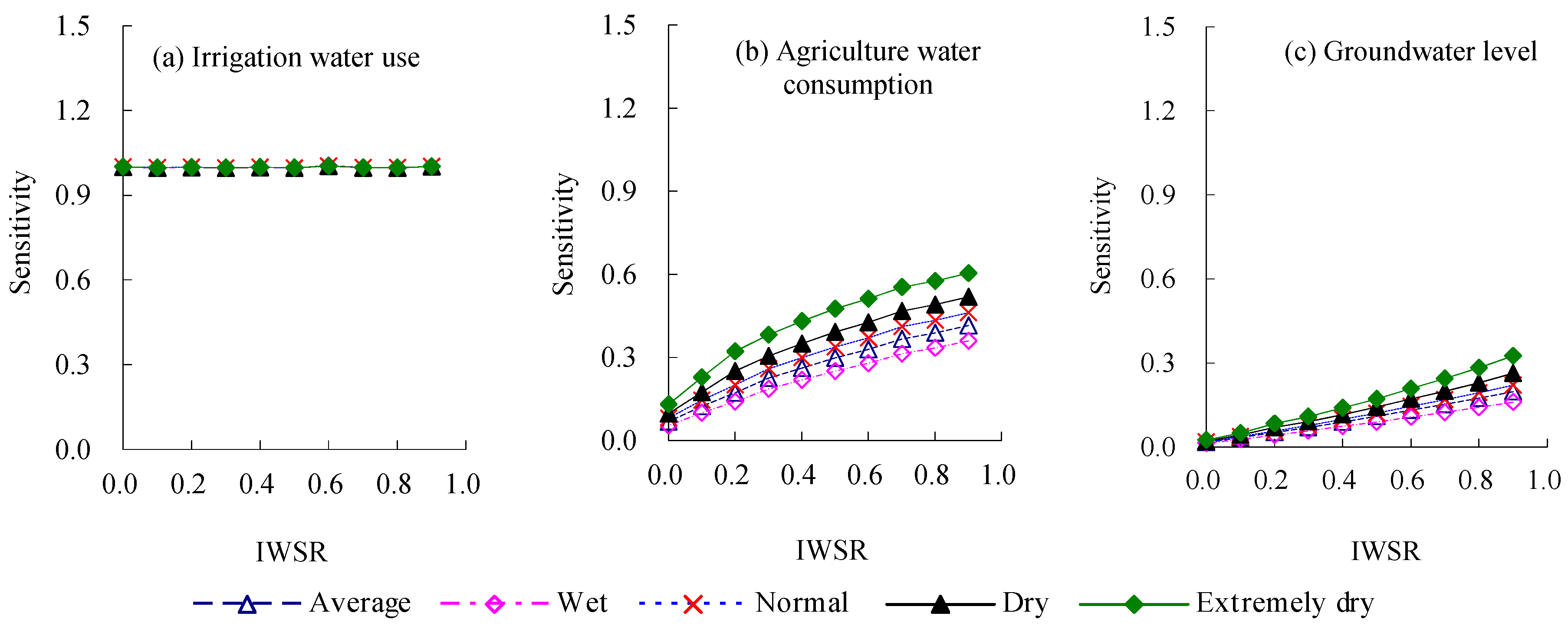
3.2.2. Sensitivity Analysis

The RD of the regional water supply and consumption to the variation of IWSR is shown in Figure 4. With the decrease of IWSR, except for the sensitivity with little change of agriculture water use, the relative sensitivity of agriculture water consumption and regional groundwater level decreases. Comparing the sensitivity of agriculture water use, agriculture water consumption, and regional groundwater level to the variation of IWSR in average years, the largest was irrigation water use at about 1.00, followed by agriculture water consumption at about 0.42 at the range of 0.9–1.0, and then regional groundwater level about 0.20 at the range of 0.9–1.0. Except for little effect of the sensitivity of irrigation water use by different hydrological years, the sensitivity of agriculture water consumption and regional groundwater level to the variation of IWSR was rather high in dry years.

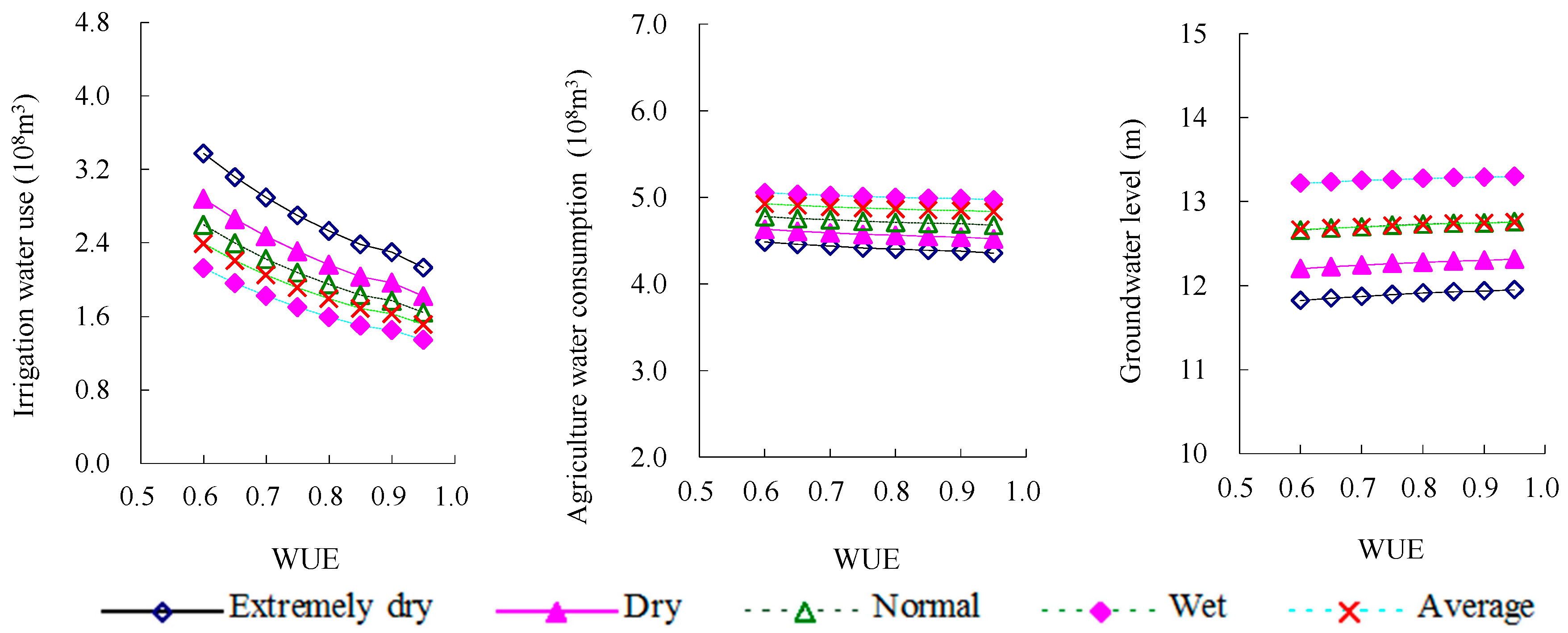
3.3. Effect of the Increase of WUE on Regional Irrigation Water Supply, Agriculture Water Consumption, and Groundwater Level

3.3.1. Variation of Regional Irrigation Water Use and Agriculture Water Consumption

The effect of the WUE increase on the regional water use and consumption is shown in Figure 5. Under IWSR of 0.8, with the increase of WUE, the decrease of irrigation water use was significant, but the decrease of agriculture water consumption and the rise of groundwater level are not obvious. For a WUE change from 0.60 to 0.95, the variation of irrigation water use, agriculture water consumption, and groundwater level with the decrease of WUE by 0.1 is shown in

Table 4. The variation of irrigation water use, agriculture water consumption and groundwater level with a decrease of WUE by 0.1.

Precipitation Type	Extremely Dry	Dry	Normal	Wet	Average
Decrease of irrigation water use (108 m3)	0.355	0.303	0.273	0.223	0.251
Decrease of agriculture water consumption (108 m3)	0.037	0.031	0.028	0.023	0.026
Raise of groundwater level (m)	0.037	0.032	0.028	0.024	0.027

. Under different hydrological years, with the increase of WUE, the water cycle components’ variation was different. With the increase of WUE, the water cycle components in dry years were affected much more than in wet years. Compared with the wet years, with the increase of WUE by 0.1 in dry years, irrigation water use decreased by about 0.132 × 10⁸ m³, agriculture water consumption decreased by about 0.014 × 10⁸ m³, and the regional groundwater level raised by about 0.013 m. With the increase of WUE, the seepage losses of irrigation water use in the canal reduced, and the withdrawal of irrigation water use decreased. Compared with the seepage losses of irrigation water use in the canal, the ineffective evaporation in the canal could be neglected, which shows that with unchanged IWSR, the decrease of agriculture water consumption was not obvious with the increase of WUE. On the other hand, the groundwater in Daxing County is recharged mainly from precipitation and seepage losses from irrigation water use. With the increase of WUE, the withdrawal of irrigation water was reduced, and the groundwater recharge from seepage of irrigation water use decreased correspondingly. So, the groundwater did not obviously decrease with the increase of WUE.

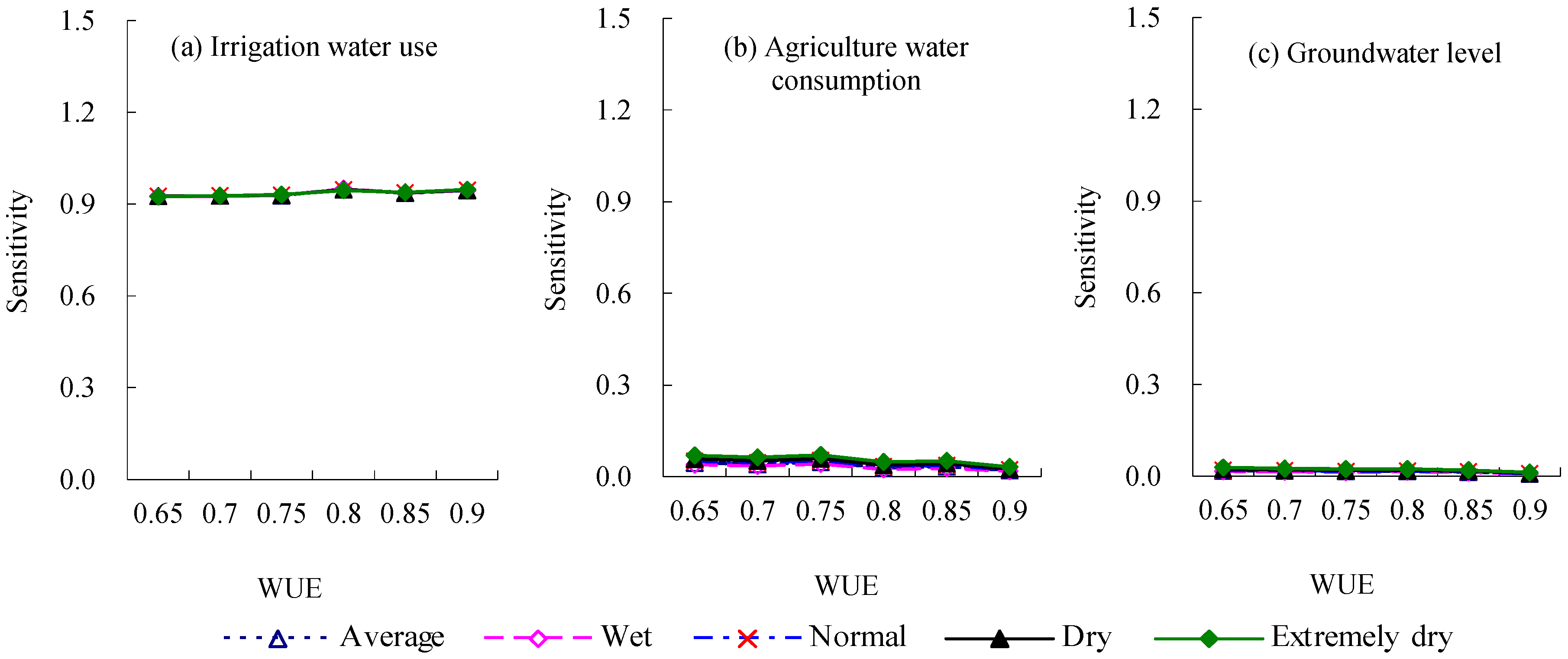
3.3.2. Sensitivity Analysis

The sensitivity of the regional water use and consumption to the variation of WUE is shown in Figure 6. With the increase of WUE, except for the sensitivity with slight increase of agriculture water use, the sensitivity of agriculture water consumption and regional groundwater level decreases. Compared with the sensitivity of agriculture water use, agriculture water consumption, and regional groundwater level to the variation of WUE in average years, the largest was irrigation water use at about 0.90 at the range of 0.60–0.90, followed by agriculture water consumption at about 0.05 at the range of 0.60–0.65, and then regional groundwater level at about 0.02 at the range of 0.60–0.65. The sensitivity of irrigation water use to the variation of WUE among different hydrological years was not obvious. Compared with the wet years, the sensitivity of agriculture water consumption and regional groundwater level to the variation of WUE was a little higher than in dry years.

3.4. Effect of Combined Measures on Regional Irrigation Water Use and Water Consumption and Its Sensitivity

3.4.1. Difference of Regional Irrigation Water Use and Water Consumption

The effect of different water management strategies on irrigation water use, agriculture water consumption, and regional groundwater level is shown in Figure 7. For different hydrological years, with the decrease of IWSR by 0.1 or the increase of WUE by 0.1, irrigation water use decreased significantly, especially with the decrease of IWSR by 0.1. With the increase of WUE by 0.1, the decrease of agriculture water consumption and the rise of regional groundwater level were affected much less than they were with the decrease of IWSR by 0.1. The variation of agriculture water consumption has a close relationship with the regime of groundwater level. With the increase of IWSR or the decrease of WUE, for an increase by 0.01 × 10⁸ m³ of agriculture water consumption, the regional groundwater level decreased 9.70 mm and 10.40 mm, respectively. So, there is no difference between them. Compared with the decrease of IWSR, with the increase of WUE, a decrease of irrigation water use has no obvious effect on the decrease of agriculture water consumption and the rise of regional groundwater level. With the increase of IWSR, for an increase by 0.01 × 10⁸ m³ of agriculture water use, agriculture water consumption increased 0.0091 × 10⁸ m³, and the groundwater level decreased 8.8 mm, which were, respectively, 9.1 and 7.6 times higher than that with the decrease of WUE under the same quantity of irrigation water withdrawal.

Therefore, how to allocate the regional water resources should be based on the variation of regional water consumption, namely the regional water consumption is the end of water resources allocation. The regional water consumption carrying capacity was not analyzed concretely for the previous water resources allocation based on water supply management, although the WUE increased by construction in agriculture production, the irrigation area increased by utilization of water-saving quantity, and the grain yield was guaranteed in short time. But due to the absence of supervision for regional water consumption, the regional water consumption was increased rapidly with the blind expansion of water-saving irrigation areas, which resulted in the continual lowering of groundwater level. Finally, the ecological balance was destroyed, which led to further deterioration of the eco-environment. On the other hand, the water-saving irrigation area was expanding constantly, while the eco-environment did not improve. In fact, once the regional total water consumption greatly exceeds the objective ET that is presently suitable for the demand between regional water balance and economic sustainability, the regional eco-environment will deteriorate. So, in order to realize the increase of agricultural production and farmers’ income, the ecological balance must be maintained. Especially in regions with water resources shortage, the total water consumption cannot exceed the objective ET quota. Only in this way will the sustainable development of agriculture be guaranteed.

3.4.2. Difference of Sensitivity

The maximum sensitivity of the regional water use and consumption to different water management strategies in average years is shown in

Table 5. The maximum sensitivity of the regional water use and consumption to different water management strategies in average years.

	Irrigation Water Use		Agriculture Water Consumption		Regional Groundwater Level
	IWSR	WUE	IWSR	WUE	IWSR	WUE
Maximum sensitivity	1.00	0.93	0.42	0.05	0.2	0.02
Value range with maximum sensitivity	0.0–1.0	0.60–0.90	0.9–1.0	0.60–0.65	0.9–1.0	0.60–0.65

. Based on sensitivity analysis, with the decrease of IWSR, the water cycle components were affected much more than they were with the increase of WUE. With the decrease of IWSR or the increase of WUE, irrigation water use and agriculture water consumption were both reduced, the regional groundwater level increased, and the sensitivity of agriculture water consumption and regional groundwater level decreased, but the sensitivity of irrigation water use remained at a high level.

4. Conclusions

With the decrease of IWSR, the irrigation water use decreased, the water consumption decreased, and the groundwater level increased, especially in dry years. The largest was the sensitivity of irrigation water use in response to the variation of IWSR, followed by agriculture water consumption, and then regional groundwater level. Except for a small effect on the sensitivity of irrigation water use by different hydrological years, the sensitivity of agriculture water consumption and regional groundwater level response to the variation of IWSR was rather high in dry years.

With the increase of WUE, the decrease of irrigation water use was significant, but the decrease of agriculture water consumption and the rise of the groundwater level were not obvious. The sensitivity analysis showed that the variations of water cycle components’ sensitivity to the increase of WUE and the decrease of IWSR are similar. Namely, the largest was the sensitivity of irrigation water use to the variation of WUE, followed by agriculture water consumption, and then regional groundwater level. On the other hand, the sensitivity of the water cycle components to the variation of WUE was a little high in dry years.

For different hydrological years, with the decrease of IWSR and the increase of WUE, irrigation water use decreased significantly, especially with the decrease of IWSR. With the increase of WUE, the decrease of agriculture water consumption and the rise of the regional groundwater level were affected much less than they were with the decrease of IWSR. The sensitivity analysis showed that with the decrease of IWSR, the water cycle components were affected much more than they were with the increase of WUE.

When the IWSR decreased through deficit irrigation, the irrigation water use and agriculture water consumption would be reduced significantly, which has more important practical significance to the sustainable utilization of regional water resources.

References

1. Bao, C.; Fang, C. Water resources constraint force on urbanization in water deficient regions: A case study of the Hexi Corridor, arid area of NW China. Ecol. Econ. 2007, 62, 508–517. [Google Scholar] [CrossRef]
2. Feng, L.; Chen, B.; Hayat, T.; Alsaedi, A.; Ahmad, B. The driving force of water footprint under the rapid urbanization process: A structural decomposition analysis for Zhangye city in China. J. Clean. Prod. 2015. [Google Scholar] [CrossRef]
3. Yan, T.; Wang, J.; Huang, J. Urbanization, agricultural water use, and regional and national crop production in China. Ecol. Model. 2015, 318, 226–235. [Google Scholar] [CrossRef]
4. Cai, M.; Wei, X.; Su, X. Influence of Irrigation Area Water Consumption Change to Ground Water Balanced. J. Irrig. Drain. 2007, 26, 16–20. (In Chinese) [Google Scholar]
5. Lei, J. Study on adjustment and control of agricultural water resource in Luohui trench irrigation district. Groundwater 2010, 32, 68–69. (In Chinese) [Google Scholar]
6. Li, Y.; Pang, H.; Chen, F.; Zhang, F.; Lai, X. Analysis on the Guarantee Degree of Irrigation Water Resources and Its Promotion Strategies in Manas River Valley, Xinjiang. J. Nat. Resour. 2010, 25, 2–42. (In Chinese) [Google Scholar]
7. Li, G.; Jia, X.; Su, X. Countermeasures of groundwater resources over-exploitation in Hebei Province. China Water Resour. 2010, 5, 36–37, 44. (In Chinese) [Google Scholar]
8. Liu, Z.; Zhang, G.; Yan, M.; Wang, J. Impact of Increases in Irrigated Grain Production on Groundwater in the Shijiazhuang Plain. Resour. Sci. 2010, 32, 535–539. (In Chinese) [Google Scholar]
9. Beijing Water Authority. Beijing Water Resources Bulletin 2014; Beijing Water Authority: Beijing, China, 2014. (In Chinese)
10. Huang, J.; Zhang, H.; Tong, W.; Chen, F. The impact of local crops consumption on the water resources in Beijing. J. Clean. Prod. 2012, 21, 45–50. [Google Scholar] [CrossRef]
11. Zhou, Y.; Wang, L.; Liu, J.; Li, W.; Zheng, Y. Options of sustainable groundwater development in Beijing Plain, China. Phys. Chem. Earth Parts A/B/C 2012, 47–48, 99–113. [Google Scholar] [CrossRef]
12. Li, Y.; Xiong, W.; Zhang, W.; Wang, C.; Wang, P. Life cycle assessment of water supply alternatives in water-receiving areas of the South-to-North Water Diversion Project in China. Water Res. 2016, 89, 9–19. [Google Scholar] [CrossRef] [PubMed]
13. Wang, Z.; Huang, K.; Yang, S.; Yu, Y. An input-output approach to evaluate the water footprint and virtual water trade of Beijing, China. J. Clean. Prod. 2013, 42, 172–179. [Google Scholar] [CrossRef]
14. Beijing Water Authority. Beijing Water Resources Bulletin 2001; Beijing Water Authority: Beijing, China, 2001. (In Chinese)
15. Cao, H.; Ge, D.; Zhao, S.; Liu, Y.; Liu, Y.; Wang, W. Evaluation for applying computer simulation in crop growth and development research. J. Triticeae Crops 2010, 30, 183–187. (In Chinese) [Google Scholar]
16. Wang, Y.; He, L. A Review on the Research and Application of Crop Simulation Model. J. Huazhong Agric. Univ. 2005, 24, 529–535. (In Chinese) [Google Scholar]
17. Xu, Z. Hydrological models: Past, Present and Future. J. Beijing Norm. Univ. Nat. Sci. 2010, 46, 278–289. (In Chinese) [Google Scholar]
18. Gopalakrishnan, M.; Mohile, A.D.; Gupta, L.N.; Kuberan, R.; Kulkarni, S.A. An integrated water assessment model for supporting India water policy. Irrig. Drain. 2006, 55, 33–50. [Google Scholar] [CrossRef]
19. Mu, J.; Khan, S.; Gao, Z. Integrated water assessment model for water budgeting under future development scenarios in Qiantang River basin of China. Irrig. Drain. 2008, 57, 369–384. [Google Scholar] [CrossRef]
20. Mu, J.; Khan, S.; Liu, Q.; Xu, D.; Xu, J.; Wang, W. A stochastic approach to analyse water management scenarios at the river basin level. Irrig. Drain. 2013, 62, 379–395. [Google Scholar] [CrossRef]
21. Mu, J.; Liu, Q.; Gabriel, H.F.; Xu, D.; Xu, J.; Wu, C.; Ren, H. The impacts of climate change on water stress situations in the Yellow River basin, China. Irrig. Drain. 2013, 62, 545–558. [Google Scholar] [CrossRef]
22. Peng, Z.; Liu, Y.; Xu, D.; Wang, L.; Zhang, B. Application of CPSP model to agricultural water management in well irrigation region in North China. J. Drain. Irrig. Mach. Eng. 2014, 32, 523–528. (In Chinese) [Google Scholar]
23. National Bureau of Statistics of China. China Statistical Yearbook 1997; National Bureau of Statistics of China: Beijing, China, 1997. (In Chinese)
24. National Bureau of Statistics of China. China Statistical Yearbook 2014; National Bureau of Statistics of China: Beijing, China, 2014. (In Chinese)
25. Peng, Z. Agricultural Water Consumption Management Studies Based on Remote sensing ET Data: A Case Study of Beijing Daxing County; China Institute of Water Resource and Hydropower Research: Beijing, China, 2009; pp. 22–24. (In Chinese) [Google Scholar]
26. Gao, Z. Study on China Food Safety and Irrigation Development Measures; China Institute of Water Resource and Hydropower Research: Beijing, China, 2005; pp. 15–22. (In Chinese) [Google Scholar]
27. Beven, K. A sensitivity analysis of the Penman-Monteith actual evapotranspiration estimates. J. Hydrol. 1979, 44, l69–190. [Google Scholar] [CrossRef]
28. Crosetto, M.; Ruiz, J.; Crippa, B. Uncertainty propagation in models driven by remotely sensed data. Remote Sens. Environ. 2001, 76, 373–385. [Google Scholar] [CrossRef]
29. Ma, J.; Yan, G.; Li, H.; Guo, S. Sensitivity and uncertainty analysis for Abreu & Johnson numericalvapor intrusion model. J. Hazard. Mater. 2016, 304, 522–531. [Google Scholar] [PubMed]
30. Mccuen, R.H. A sensitivity and error analysis of procedures used for estimating evaporation. Water Resour. Bull. 1974, 10, 486–498. [Google Scholar] [CrossRef]
31. Médard, B.; Alain, N.R.; Silvio, J.G.; Patrick, G.; Brou, K.; Roger, M. Implementation of an automatic calibration procedure for HYDROTEL based on prior OAT sensitivity and complementary identifiability analysis. Hydrol. Process. 2014, 28, 3947–3961. [Google Scholar]
32. Cai, X.; Xu, Z.; Su, B.; Yu, W. Distributed simulation for regional evapotranspiration and verification by using remote sensing. Trans. CSAE 2009, 25, 154–160. (In Chinese) [Google Scholar]
33. Immerzeel, W.W.; Droogers, P. Clibration of a distributed hydrological model based on satellite evapotranspiration. J. Hydrol. 2008, 349, 411–424. [Google Scholar] [CrossRef]
34. Peng, Z.; Mao, D.; Wang, L.; Liu, Y.; Zhang, J. Establishment of the regional water balance analysis model based on RS ET data and current situation analysis. J. Remote Sens. 2011, 15, 313–317. [Google Scholar]
35. Wu, B.; Yan, N.; Xiong, J.; Bastiaanssen, W.G.M.; Zhu, W.; Stein, A. Validation of ETWatch using field measurements at diverse landscapes: A case study in Hai Basin of China. J. Hydrol. 2012, 436–437, 67–80. [Google Scholar] [CrossRef]
36. Wu, B.; Xiong, J.; Yan, N. ETWatch: Models and methods. J. Remote Sens. 2010, 15, 224–230. [Google Scholar]
37. Wu, B.; Xiong, J.; Yan, N.; Yang, L.; Du, X. ETWatch for monitoring regional evapotranspiration with remote sensing. Adv. Water Sci. 2008, 19, 671–678. [Google Scholar]
38. Kahimba, F.C.; Bullock, P.R.; Sri-Ranjan, R.; Cutforth, H.W. Evaluation of the SolarCalc model for simulating hourly and daily incoming solar radiation in the Northern Great Plains of Canada. Can. Biosyst. Eng. 2009, 51, 1–11. [Google Scholar]
39. Willmott, C.J. Some comments on the evaluation of model performance. Bull. Am. Meteorol. Soc. 1982, 63, 1309–1313. [Google Scholar] [CrossRef]
40. Willmott, C.J.; Maasuura, K. Advantages of the meanabsolute error (MAE) over the root mean square error (RMSE) in assessing average model performance. Clim. Res. 2005, 30, 79–82. [Google Scholar] [CrossRef]
Figure 1. Comparison between the calculated value and the observer value for model calibration. (a) Comparison of calculated evapotranspiration (ET) to remote sensing ET (RS ET) for different land use in 2004; (b) Linear relationship between RS ET and calculated ET for all the land use.
Sustainability 08 00749 g001
Figure 2. Comparison between the calculated value and the observer value for model validation. (a) Comparison of calculated ET to RS ET for different land use in 2005; (b) Linear relationship between RS ET and calculated ET for all the land use.
Sustainability 08 00749 g002
Figure 3. The effect of the decrease of IWSR on the regional water use and consumption.
Sustainability 08 00749 g003
Figure 4. The sensitivity of the regional water use and consumption compared to the variation of IWSR. (a) Irrigation water use; (b) Agriculture water consumption; (c) Groundwater level.
Sustainability 08 00749 g004
Figure 5. The effect of the WUE increase on the regional water use and consumption.
Sustainability 08 00749 g005
Figure 6. The sensitivity of the regional water use and consumption to the variation of WUE. (a) Irrigation water use; (b) Agriculture water consumption; (c) Groundwater level
Sustainability 08 00749 g006
Figure 7. The effect of different water management strategies on irrigation water use, agriculture water consumption, and regional groundwater level.
Sustainability 08 00749 g007