An Impact Analysis of Farmer Field School in China

Abstract

In this paper, we investigate the impact of the Farmer Field School (FFS) intervention among small-scale tomato farmers in Beijing. Using data collected by face-to face-interview from 358 households on 426 planting plots in 2009, we evaluate the yield effect and find evidence of positive impact. We then examine the determining factors of farmers’ FFS attendance using the zero-inflated Poisson model. We find evidence of the positive impact of the FFS program on male participants but no impact on female participants. We find that some factors, such as being the household head, wealth level and land size affect both FFS participation decisions and attendance decisions, whereas other factors may affect only one decision but not the other. The results suggest that FFS is a useful way to increase production of farmers in Beijing and that the approach is especially effective for male and wealthy producers with smaller farm sizes and higher literacy.

1. Introduction

Farmer field school (FFS) was first promoted by the Food and Agriculture Organization (FAO) in Indonesia in a small scale rice-based system in 1989–1990 and then quickly expanded to other Asian and African countries [1,2,3,4,5]. As a new agricultural extension approach, FFS was initially used to diffuse the knowledge-intensive integrated pest management (IPM) concepts to solve the problem of insecticide overuse in irrigated rice systems in Asia [6,7]. Unlike the traditional top-down extension approaches, the FFS were developed as a “bottom-up” approach and focused on both the training and the farmer-to-farmer diffusion [8,9]. All FFS participants are encouraged to discuss and share their experiences with other farmers in the training class, as well as with people within their local villages and community organizations [10]. Because farmers often rely on their neighbors for information and advice, the farmer-to-farmer approach makes it easier for farmers to accept and adopt the new knowledge and technologies [11]. Farmers act not only as instructors but also as facilitators which can help farmers “to develop their analytical skills, critical thinking, and creativity, and help them learn to make better decisions” [12,13].

Studies have found evidence of FFS effectiveness in production, pesticide use, and knowledge diffusion [14,15,16]. As a result, the FAO and a number of international development agencies, such as the World Bank, have subsidized the FFS program in developing countries since the 1990s [6,17]. The World Bank has been promoting the FFS as the “most effective approach” in knowledge and technology diffusion [9].

Many studies have assessed the impact of FFS by dividing people into FFS and non-FFS groups [14,15,16]. However, no study examined the impact of the intensity of farmers’ FFS attendance. If farmers benefit from attending the FFS and sharing discussions with other attendees, then the more frequently they attend, the stronger the impact would be. In most of the existing FFS literature, there are usually a fixed number of training sessions and the attendance of farmers is compulsory [6,7,11,14]. In this study, we examined the impact of a multiple-year FFS program introduced in Beijing in 2005. Training sessions are provided approximately 14 times a year. Participating farmers can choose to attend or not attend any given session. This provides us with a viable venue to investigate the impact of the intensity of FFS attendance.

We are also interested in whether a gender effect exists for FFS attendance behavior since study has found that the FFS was more beneficial to female farmers than to male farmers in raising their crop productivities [18]. In this paper, first, we will use the attendance of male and female farmers to measure the impact of FFS on tomato production. Then, we will attempt to find the determinants of farmers’ attending FFS to gain insights into how to encourage greater attendance. As mentioned above, several studies have estimated the impact of FFS on yield, but most of them have used a “with-program and without-program” framework for comparison [19]. None have considered using the FFS session attendance as a measure to estimate the training effects. In this study, we will assess the impact of FFS training on productivity using the attendance as a measure of the training intensity. To distinguish the effect of FFS training by gender, we will use the attendance of male and female farmers separately.

The paper is organized as follows. Section 2 describes the FFS program in Beijing. Section 3 presents the methodology and materials. Section 4 presents the data and summary statistics. In Section 5 we outline the empirical models and then discuss the results: the impact of FFS on the production in Section 6 and the determinants of farmers’ FFS attendance in Section 7. Section 8 provides conclusions and implications.

2. The Farmer Field Schools Program in Beijing

The FAO-supported FFS programs were launched nationwide in China in the 1990s, but were largely discontinued in 2007 due to FAO’s cutoff of funding support [20,21]. In 2005, the local government of Beijing initiated a long term FFS program via the agricultural extension system to introduce the IPM concept to farmers.

The FFS program in Beijing is the first that is fully funded by the local government. The implementation of the FFS program was written into the local government document. It has been interpreted as a paradigm shift from an externally supported project into an internally sustainable development mechanism. By 2010, 758 FFSs were set up in Beijing, one in each participating village. They include 20% of all the agricultural villages in the Beijing area. Approximately 40,000 farmers participate in the FFSs’ activities.

3. Methodology and Materials

The farmers recruited in the FFS group (so-called FFS members) are not forced to take the sessions. A few of them never showed and some of them took only some sessions, but not all. Meanwhile, some of the non-FFS member farmers also attended the training sessions because the FFS classes were open to all farmers. In this case, the traditional approach of dividing farmers into FFS members and non-FFS members would lead to biased estimates of the effect of FFSs because some non-FFS member farmers also received the training.

To address this issue, we define the FFS and non-FFS farmers using their attendance at sessions instead of the nominal FFS membership. If a farmer never showed up to any session, she will be viewed as a non-FFS farmer. Otherwise, she will be a FFS farmer. Accordingly, we use the number of sessions attended instead of a dummy of FFS membership in the analysis.

In this study, we examine the tomato FFS because it accounts for 28.1% of all the FFSs in Beijing. We collected the data via face-to-face interviews by questionnaires with structured questions. The interview was conducted with the person mainly responsible for agricultural decisions in each household and the enumerators were well trained before the interview. We interviewed the tomato farmers in 16 villages from four randomly chosen counties in Beijing in 2009. These four counties account for approximately 90% of the large-scale tomato production in Beijing. Within each county two treatment villages with the FFS were established, and two control villages were randomly selected because there are only a few of non-FFS farmers in the FFS village. Within each FFS village, we interviewed at most 20 FFS member farmers and 20 non-FFS member farmers, all randomly chosen whenever the population was more than 20 in each group. Indeed the number of non-FFS farmers in the FFS village is usually less than 10; thus, we interviewed virtually all of them. In the control non-FFS villages, we also interviewed at most 20 randomly selected tomato farmers whenever the population was more than 20.

In each household, we collected the production information for up to two randomly chosen planted tomato varieties. In total, we obtained information on 435 planting plots from 365 households in the 16 villages. Of the 365 households, seven were headed by a single male or female. In this study, we include only the non-single head households as we would like to use the spouse’s information as part of the explanatory variables. Therefore, we dropped these seven households from our analysis, leaving 426 plots from 358 households. Of all these plots, 274 plots were from 229 households in the FFS villages, and the remainders were from the non-FFS villages.

4. The Data and Summary Statistics

Because both participation and training attendance are voluntary, people may self-select in making these decisions, leading to self-selection problems. For example, more motivated farmers may attend more. If so, this could result in a positive selection effect. If farmers attended more because they were unskilled with technologies and thus had a higher demand for technology training, this could result in a negative selection effect.

To find evidence of possible self-selection behavior, we conduct a t-test between the FFS farmers and non-FFS farmers for their household characteristics. The results are shown in Table 1. There is no significant difference between the two groups in terms of family size, the gender of the household head, the educational achievement of the household head, the household head’s fraction of farming time (defined as Annual farming time/Total annual work time), the off-farm labor ratio (defined as Number of off-farm labor/Total number of household labor), and the value of assets per capita. However, farmers who attended the FFS training were approximately two years younger than those who did not: 47.7 vs. 50. One possible reason is that younger farmers may have less farming experience and thus have more demand for technologies. If so, this may suggest a negative selection effect.

Table 1. Comparison of household characteristics between farmer field school (FFS) group and non-FFS group.

Characteristics	Mean ± SD		p-Value
	FFS Group	Non FFS Group
Family size (number of family members)	3.79 ± 1.23	3.66 ± 1.27	0.30
Age of household head (years)	47.69 ± 7.54	50.24 ± 7.19	0.00
Household head is male	0.79 ± 0.41	0.76 ± 0.43	0.47
Education of household head (years)	8.70 ± 2.18	8.61 ± 2.12	0.66
Fraction of farming time of household head (%)	94.42 ± 19.19	96.01 ± 16.94	0.37
Fraction of labors off the farm (%)	43.36 ± 0.21	42.32 ± 0.24	0.63
Per capita fixed assets (thousand yuan)	105.17 ± 156.54	112.63 ± 178.44	0.65
Observations	229	197

Note: SD refers to the standard deviation. Source: authors’ own survey.

Table 1. Comparison of household characteristics between farmer field school (FFS) group and non-FFS group.

Characteristics	Mean ± SD		p-Value
	FFS Group	Non FFS Group
Family size (number of family members)	3.79 ± 1.23	3.66 ± 1.27	0.30
Age of household head (years)	47.69 ± 7.54	50.24 ± 7.19	0.00
Household head is male	0.79 ± 0.41	0.76 ± 0.43	0.47
Education of household head (years)	8.70 ± 2.18	8.61 ± 2.12	0.66
Fraction of farming time of household head (%)	94.42 ± 19.19	96.01 ± 16.94	0.37
Fraction of labors off the farm (%)	43.36 ± 0.21	42.32 ± 0.24	0.63
Per capita fixed assets (thousand yuan)	105.17 ± 156.54	112.63 ± 178.44	0.65
Observations	229	197

Note: SD refers to the standard deviation. Source: authors’ own survey.

The definition and summary statistics for the variables used in this study are presented in Table 2. The average tomato yield was 70,159 kilos/ha, and the average attendance of each household was 4.15. The average attendances of male and female farmers were 2.45 and 1.70, respectively. Approximately 55% of the tomatoes were planted in the fall. Cherry tomatoes account for only 4% of all the tomatoes planted. On average, each household had 3.73 members, with assets per capita at RMB 108.6 thousand (equivalent to US$17,000). Seventy-seven percent of the household heads were male. The average age of the household head was 48.9, with 8.66 years of education completed, which is equivalent to the completion of junior high school. The household heads spent 95% of their working time on farming activities. Only 5% of the household heads held a village cadre position. For the input variables, the average labor days were 1514 days/ha, and the machinery expenditure was 656 yuan/ha. On average, farmers applied 463 kilos/ha of nitrogen fertilizer, 309 kilos/ha of phosphorus fertilizer and 376 kilos/ha of kalium fertilizer to their tomato fields. The quantity of pesticides used was 38.46 kilos/ha and they irrigated the fields approximately 8.8 times during the planting season.

Table 2. Definition of variables and summary statistics.

Variable	Definition	Mean	Std. Dev	Min	Max
Yield	Yield (kg/ha)	70,159.54	23,500.35	13,500	135,000
FFSA_household	Each household’s attendance in FFS (in number)	4.15	5.85	0	28
FFSA_male	Husband’s attendance in FFS (in number)	2.45	4.39	0	14
FFSA_female	Wife’s attendance in FFS (in number)	1.70	3.81	0	14
Fall	Dummy variable for fall	0.55	0.50	0	1
Cherry	Dummy variable for cherry tomato	0.04	0.20	0	1
Household Characteristics
Fsize	Family size	3.73	1.25	1	8
Hhdgender	Dummy variable for male household head	0.77	0.42	0	1
Hhage	Age of the household head (years)	48.87	7.48	26	72
Hhedu	Education of household head (years)	8.66	2.15	0	16
Cadre	Dummy variable for household head is a village cadre	0.05	0.23	0	1
Hfarm	Fraction of farming time of household head (in % of whole working time)	95.16	18.18	0	100
Offlab	Fraction of labors off the farm (%)	43	22	0	100
Passet	Per capita fixed assets (1000yuan/person)	108.62	166.87	1.8	1451.83
Input Variables
Labor	Labor (day/ha)	1513.98	831.61	268.36	9250
Machine	Machine (yuan/ha)	655.69	656.64	0	4200
N	Pure nitrogen (kilos/ha)	463.36	410.38	0	3153.13
P	Pure phosphorus (kilos/ha)	308.75	498.72	0	9143.75
K	Pure kalium (kilos/ha)	375.53	411.74	0	2981.25
Qpest	Quantity of pesticides (kilos/ha)	38.46	36.71	0	237
Nirri	Number of irrigations	8.84	4.81	2	35

Source: authors’ own survey.

Table 2. Definition of variables and summary statistics.

Variable	Definition	Mean	Std. Dev	Min	Max
Yield	Yield (kg/ha)	70,159.54	23,500.35	13,500	135,000
FFSA_household	Each household’s attendance in FFS (in number)	4.15	5.85	0	28
FFSA_male	Husband’s attendance in FFS (in number)	2.45	4.39	0	14
FFSA_female	Wife’s attendance in FFS (in number)	1.70	3.81	0	14
Fall	Dummy variable for fall	0.55	0.50	0	1
Cherry	Dummy variable for cherry tomato	0.04	0.20	0	1
Household Characteristics
Fsize	Family size	3.73	1.25	1	8
Hhdgender	Dummy variable for male household head	0.77	0.42	0	1
Hhage	Age of the household head (years)	48.87	7.48	26	72
Hhedu	Education of household head (years)	8.66	2.15	0	16
Cadre	Dummy variable for household head is a village cadre	0.05	0.23	0	1
Hfarm	Fraction of farming time of household head (in % of whole working time)	95.16	18.18	0	100
Offlab	Fraction of labors off the farm (%)	43	22	0	100
Passet	Per capita fixed assets (1000yuan/person)	108.62	166.87	1.8	1451.83
Input Variables
Labor	Labor (day/ha)	1513.98	831.61	268.36	9250
Machine	Machine (yuan/ha)	655.69	656.64	0	4200
N	Pure nitrogen (kilos/ha)	463.36	410.38	0	3153.13
P	Pure phosphorus (kilos/ha)	308.75	498.72	0	9143.75
K	Pure kalium (kilos/ha)	375.53	411.74	0	2981.25
Qpest	Quantity of pesticides (kilos/ha)	38.46	36.71	0	237
Nirri	Number of irrigations	8.84	4.81	2	35

Source: authors’ own survey.

5. Specification of the Empirical Model

The economic impact of FFS is estimated using the following specification:

$$Y=f(FFS{A}_{male},FFS{A}_{female},Fall,Cherry,County,Z,O)$$

(1)

where Y is the tomato yield of each plot; $FFS{A}_{male}$ is the attendance of the male household member (all were the husband); $FFS{A}_{female}$ is the attendance of the female household member (all were the wife); Fall is a dummy variable representing whether the tomato is planted in the fall or in the spring (=1 if in the fall; zero if in the spring); Cherry is also a binary variable representing whether or not cherry tomatoes were planted (=1 if yes; zero otherwise); County will capture the county specific fixed effect; Z is a vector of observable household characteristics; and O includes other input variables. For Z, we have family size, off-farm labor ratio, assets per capita, and major demographics of the household head, including gender, age, educational achievement, village cadre or not, and fraction of farming time. Other input variables are the number of labor days, the machinery expenditure, the amounts of fertilizer and pesticides applied, and the amount of irrigation conducted. The choices of control covariates are consistent with those in the existing empirical studies of FFS impact [9,14].

It follows that Equation (1) can be written as a regression model for the i-th household:

$$Y_i=\alpha +FFS{A}_{i.male}+FFS{A}_{i,female}+Fal{l}_i+Cherr{y}_i+Count{y}_i+\mathsf{\gamma }\cdot Z_i+\mathsf{\tau }\cdot O_i+{\epsilon }_i$$

(2)

where α, 𝛾, and 𝜏 are parameters to be estimated, and ε is the random error. We use the ordinary least square (OLS) approach to estimate Equation (2).

In order to detect the possible selection effect, we will also use the attendance of each household instead of the attendance of male and female farmers, and then use an instrument variable to correct the possible selection bias. This regression model for the i-th household is specified as follow:

$$Y_i=\alpha +FFS{A}_{i.household}+Fal{l}_i+Cherr{y}_i+Count{y}_i+\mathsf{\gamma }\cdot Z_i+\mathsf{\tau }\cdot O_i+{\epsilon }_i$$

(3)

where $FFS{A}_{i,household}$ is the attendance for the i-th household. Other variables are the same as mentioned above. We will use the share of trained farmers in a neighboring village as an instrument variable (IV). Since the share of trained farmers in a neighboring village is independent from the characteristics of farmers in this village, it satisfies the first condition of instrument variable that the IV should be an exogenous variable. It is apparent the participation behavior of spatially adjacent zones correlate with each other, as they share similar environmental and market characteristics [22]. Hence the share of trained farmers in a neighboring village will have positive impact on farmer’s attendance in FFS which satisfies the second condition of instrument variable that the IV should correlates with the endogenous variable. Thus the share of trained farmers in a neighboring village may serve as a good instrument for the FFS attendance of each household.

The Zero-Inflated Poisson Model

The second model is to estimate the determinants of farmers’ attendance of the FFS. The dependent variable of the model is the number of sessions attended, which is a count variable. The ordinary least square method is no longer an appropriate method. A commonly used method for the analysis of count data is the Poisson model [23,24,25]. Following Wooldridge [26], the probability that the attendance of farmers (A) equals a, conditional on $x$, is

$$\mathrm{Pr}\left(A=a|x\right)=\frac{e^{-\exp \left(x\beta \right)}{[\exp (x\beta )]}^a}{a!},a=0,1,2,\mathrm{...}$$

(4)

where $x$ is a vector of potential determinants of farmers’ attendance decisions, and $\beta$ is a parameter to be estimated.

One limitation of using the Poisson model is that the variance of the data is restricted to be equal to the mean [27,28,29]: $E(a_i|x_i)=Var(a_i|x_i)=u_i$. In many empirical applications of the model, the variance of the count data was found to be larger than the mean [27,28,29,30,31]. Ignoring the extra variations would lead to the underestimation of the variance of the estimated parameters [30]. To address this limitation, Wedderburn [31] suggests coding the variance of $a_i$ as $\phi u_i$ instead, where φ ≥ 1 is an over-dispersion parameter. This model is called the negative binomial model. It can be used to address the over-dispersion problem in count data.

Another limitation of the Poisson model is its failure to fit the data with a large frequency of “extra” zeros in the distribution. In our study, we record the attendance of male and female farmers separately. The zero attendance by one spouse may be because he/she may live away from the family and thus cannot go to the training session. We use the zero-inflated Poisson (ZIP) model to address this issue. In the ZIP model, the observations with zeros arise in two ways, corresponding to distinct underlying states [32]. The first state occurs with probability p and produces only zeros, whereas the other state occurs with probability 1 − p and leads to a standard Poisson distribution with mean ${\mathsf{\lambda }}_{\mathrm{i}}$.

In general, the zeros from the first state are called structural zeros, and those from the second state are called sampling zeros [24,33]. The probability mass function for the ZIP models is as follows:

$$f(a_i,{\lambda }_i,p)=\{\begin{array}{l}p+(1-p)e^{-{\lambda }_i}, a_i=0\\ \left(1-p\right)\frac{e^{-{\lambda }_i}{{\lambda }_i}^{a_i}}{a_i!}, a_i=1,2,\mathrm{...}\end{array}$$

(5)

where 0 ≤ p ≤ 1. The mean and variance of the ZIP random variable are:

$$E(A_i)=(1-p){\lambda }_i$$

$$Var(A_i)=(1-p){\lambda }_i+p(1-p){\lambda }_i^2$$

When $p=0$, the ZIP regression model is reduced to the Poisson regression model. When $p>0$, it follows that variance of $Y_i$ exceeds its mean. Thus, the ZIP model allows over-dispersion in the data due to excess zeros. In our data, the proportions of zeros for the male and female farmers are, respectively, 43.2% and 63.8%.

For applying the ZIP model in practical modeling, Lambert suggested the following joint models for $p$ and $\lambda$ [34]:

$$Logit\left(p\right)=\text{log}\left(\frac{p}{1-p}\right)=G\mathsf{\delta } \text{and} \text{log}\left(\mathsf{\lambda }\right)={X}\mathsf{\beta }$$

(6)

where G and X are covariate matrices, and δ, β are vectors of unknown parameters. In this paper, our ZIP model is specified as follows:

$$\log \left(\frac{p}{1-p}\right)={\mathsf{\delta }}_0+X_1{\mathsf{\delta }}_1+X_2{\mathsf{\delta }}_2+X_3{\mathsf{\delta }}_3+X_4{\mathsf{\delta }}_4+X_5{\mathsf{\delta }}_5+\mathsf{\xi }$$

$$\log \left(\mathsf{\lambda }\right)=\log (\frac{E(A_i)}{1-p})={\beta }_0+X_1{\beta }_1+X_2{\beta }_2+X_3{\beta }_3+X_4{\beta }_4+X_5{\beta }_5+\mathsf{\mu }$$

(7)

where $X_1$ is a dummy variable of whether the husband/wife is the household head. $X_2$ is a vector of a “husband’s characteristics” including his age, his square of age, his education, and his fraction of farming time. $X_3$ is a vector of a “wife’s characteristics” including her age, her square of age, her education, and her fraction of farming time. $X_4$ is a vector of “household characters” including family size, number of kids and per capita fixed assets. $X_5$ is a dummy variable of whether the land scale is small. $\mathsf{\xi }$ and $\mathsf{\mu }$ are the error terms. The definitions of these variables are listed in Table 3. The independent variables are the attendance of the husband or wife.

Table 3. Definitions of variables used in the zero-inflated models.

Household Head	Dummy Variable for Household Head	Landsmall	Dummy Variable for Land Area is Less Than Median
age_hus	Age of husband (in years)	farmtime_wife	Fraction of farming time of wife
age square _hus	Square of age of husband	family size	Number of family members
education_hus	Education of husband (years)	number of kids	Number of kids that are younger than or equal to six years old
farmtime_hus	Fraction of farming time of husband	passets	Per capita fixed assets (million yuan)
age_wife	Age of wife (years)	education_wife	Education of wife (years)
age square_wife	Square of age of wife

Table 3. Definitions of variables used in the zero-inflated models.

Household Head	Dummy Variable for Household Head	Landsmall	Dummy Variable for Land Area is Less Than Median
age_hus	Age of husband (in years)	farmtime_wife	Fraction of farming time of wife
age square _hus	Square of age of husband	family size	Number of family members
education_hus	Education of husband (years)	number of kids	Number of kids that are younger than or equal to six years old
farmtime_hus	Fraction of farming time of husband	passets	Per capita fixed assets (million yuan)
age_wife	Age of wife (years)	education_wife	Education of wife (years)
age square_wife	Square of age of wife

6. Results: The Impact of FFS on Farmers’ Tomato Yield

Table 4 presents the estimation results of Equation (2). Column (1) presents the logarithm regression of tomato yield for the complete set of regressors, and column (3) present the results without the variety and input variables. Columns (2) and (4) present the corresponding t values. All regressions are conducted with robust standard errors clustered at village level to accommodate the potential heterogeneity issue.

Table 4. Impact of male and female’s attendance in farmer field school on tomato yields.

Variables	(1) Log(yield)	(2) t-value	(3) Log(yield)	(4) t-value
FFSA_male	0.0153 ***	3.22	0.0157 **	2.88
FFSA_female	0.006	0.87	0.00710	0.96
Fall	−0.179 ***	−4.21	−0.178 ***	−4.05
Log(fsize)	−0.047	−0.68	−0.071	−1.03
Hhdgender	−0.041	−0.67	−0.035	−0.57
Log(hhage)	−0.046	−0.46	−0.015	−0.13
Log(hhedu)	0.008	0.67	0.013	1.20
Cadre	−0.040	−0.38	−0.061	−0.54
Hfarm	0.001	1.29	0.001	0.91
Offlab	0.0007	0.43	0.0007	0.49
Log(passet)	0.027 **	2.25	0.027 **	2.24
Cherry	−0.184 ***	−3.10	-	-
Log(labor)	0.102 ***	3.00	-	-
Log(machine)	0.002	0.82	-	-
Log(n)	−0.003	−0.58	-	-
Log(p)	0.002	0.32	-	-
Log(k)	−0.006	−1.03	-	-
Log(qpest)	−0.011	−1.51	-	-
Log(nirri)	0.077 **	2.24	-	-
Constant	9.838 ***	24.12	10.62 ***	21.08
Observations	426	-	426	-
R-squared	0.260	-	0.225	-

Note: County dummy variables are included in the regression but are not reported for the sake of simplicity. ***, **, * indicate statistically significant at 1%, 5% and 10%, respectively. Source: authors’ own survey.

Table 4. Impact of male and female’s attendance in farmer field school on tomato yields.

Variables	(1) Log(yield)	(2) t-value	(3) Log(yield)	(4) t-value
FFSA_male	0.0153 ***	3.22	0.0157 **	2.88
FFSA_female	0.006	0.87	0.00710	0.96
Fall	−0.179 ***	−4.21	−0.178 ***	−4.05
Log(fsize)	−0.047	−0.68	−0.071	−1.03
Hhdgender	−0.041	−0.67	−0.035	−0.57
Log(hhage)	−0.046	−0.46	−0.015	−0.13
Log(hhedu)	0.008	0.67	0.013	1.20
Cadre	−0.040	−0.38	−0.061	−0.54
Hfarm	0.001	1.29	0.001	0.91
Offlab	0.0007	0.43	0.0007	0.49
Log(passet)	0.027 **	2.25	0.027 **	2.24
Cherry	−0.184 ***	−3.10	-	-
Log(labor)	0.102 ***	3.00	-	-
Log(machine)	0.002	0.82	-	-
Log(n)	−0.003	−0.58	-	-
Log(p)	0.002	0.32	-	-
Log(k)	−0.006	−1.03	-	-
Log(qpest)	−0.011	−1.51	-	-
Log(nirri)	0.077 **	2.24	-	-
Constant	9.838 ***	24.12	10.62 ***	21.08
Observations	426	-	426	-
R-squared	0.260	-	0.225	-

Note: County dummy variables are included in the regression but are not reported for the sake of simplicity. ***, **, * indicate statistically significant at 1%, 5% and 10%, respectively. Source: authors’ own survey.

Results in column (1) in Table 4 suggest that the attendance of FFS sessions is positively associated with tomato yield for male farmers. On average, attending one more session is associated with a 1.53% yield increase. On average, male FFS farmers attended 4.7 training sessions. It may suggest a corresponding yield increase of 7.19%. The coefficient of the attendance by female FFS farmers in the household is statistically insignificant. This result differs from that of Davis [18], who found that the FFSs were more beneficial to women than to men. Note that the average attendance of women in the FFS in our sample is lower than that of men as follows: 3.0 versus 4.7, on average. Given that there are a total of 14 sessions offered, neither group showed a high attendance rate. The low attendance rate may suggest that farmers are not always ready for these types of trainings. Our results on the positively significant coefficient of the FFS attendance could lead to policy recommendations for encouraging FFS attendance by farmers.

The production of tomatoes in fall is 17.9% lower than in spring. The yield of cherry tomatoes is 18.4% lower than of other varieties. Most of the household characteristics are not statistically significant, except for the per capita fixed assets. Households with higher per capita assets tend to observe higher tomato yields. For the input variables, labor has a positive effect on tomato production, and more irrigation may result in higher tomato yields.

Column (3) presents the results of the impact of FFS on tomato yield without variety and input variables. The result in column (3) is similar to those in column (1): the attendance of FFS sessions is positively associated with tomato yield for male farmers, and the coefficient of the attendance by female FFS farmers is statistically insignificant. Since the coefficient of male farmers’ attendance is almost the same with that in column (1), we can hardly say that there would be any variety and input choice effect in the FFS training.

The effect of attendance in FFS in Table 4 may be downward biased because of self-selection problem. It is difficult for us to find two valid instrument variables to correct the self-selection problem in Equation (2). Instead we use the attendance of each household as an independent variable and the share of trained farmers in a neighboring village as the instrument variable to address the selection bias. Table 5 presents the estimation results of Equation (3). Column (1) and (2) present the logarithm regression of tomato yield with the OLS approach, and column (3) and column (4) present the corresponding results with a two stage least square (2SLS) approach.

Table 5. Impact of household’s attendance in farmer field school on tomato yield.

Variables	(1) Lyield (OLS)	(2) Lyield (OLS)	(3) Lyield (2SLS)	(4) Lyield (2SLS)
FFSA_household	0.011 ***	0.012 **	0.021 ***	0.021 ***
	(0.004)	(0.005)	(0.006)	(0.007)
Fall	−0.172 ***	−0.172 ***	−0.189 ***	−0.190 ***
	(0.047)	(0.050)	(0.043)	(0.044)
Log(fsize)	−0.045	−0.068	−0.061	−0.082
	(0.067)	(0.066)	(0.060)	(0.060)
Hhdgender	−0.017	−0.013	−0.017	−0.012
	(0.056)	(0.057)	(0.053)	(0.056)
Log(hhage)	−0.052	−0.027	−0.018	−0.002
	(0.104)	(0.127)	(0.089)	(0.106)
Log(hhedu)	0.007	0.013	0.008	0.012
	(0.011)	(0.011)	(0.010)	(0.010)
Cadre	−0.035	−0.057	−0.052	−0.070
	(0.099)	(0.106)	(0.094)	(0.105)
Hfarm	0.0013	0.001	0.0014	0.0012
	(0.001)	(0.001)	(0.001)	(0.001)
Offlab	0.0008	0.0008	0.0009	0.0009
	(0.0015)	(0.0014)	(0.0014)	(0.0014)
Log(passet)	0.030 **	0.029 **	0.029 **	0.028 **
	(0.013)	(0.013)	(0.012)	(0.012)
Cherry	−0.178 ***	-	−0.157 *	-
	(0.060)	-	(0.081)	-
Log(labor)	0.104 ***	-	0.103 ***	-
	(0.035)	-	(0.037)	-
Log(machine)	0.0025	-	0.0023	-
	(0.003)	-	(0.003)	-
Log(n)	−0.003	-	0.0001	-
	(0.006)	-	(0.005)	-
Log(p)	0.0025	-	0.0009	-
	(0.007)	-	(0.006)	-
Log(k)	−0.006	-	−0.006	-
	(0.006)	-	(0.005)	-
Log(qpest)	−0.011	-	−0.012 *	-
	(0.007)	-	(0.007)	-
Log(nirri)	0.070 *	-	0.057 *	-
	(0.034)	-	(0.029)	-
Constant	9.798 ***	10.60 ***	9.643 ***	10.47 ***
	(0.405)	(0.496)	(0.399)	(0.420)
Observations	426	426	426	426
R-squared	0.255	0.221	0.235	0.205
Instrument Variable test (first stage)
Share of trained farmers in a neighboring village	-	-	0.080 ***	0.078 ***
	-	-	(0.010)	(0.010)
Cragg-Donald Wald F Statistic	-	-	157.07	151.72
10% Stock-Yogo weak ID test critical value	-	-	16.38	16.38

Note: County dummy variables are included in the regression but are not reported for the sake of simplicity. Other exogenous variables are not reported in the IV test. Standard errors are robust and clustered at village level in all regressions. ***, **, * indicate statistically significant at 1%, 5% and 10%, respectively. Source: authors’ own survey.

Table 5. Impact of household’s attendance in farmer field school on tomato yield.

Variables	(1) Lyield (OLS)	(2) Lyield (OLS)	(3) Lyield (2SLS)	(4) Lyield (2SLS)
FFSA_household	0.011 ***	0.012 **	0.021 ***	0.021 ***
	(0.004)	(0.005)	(0.006)	(0.007)
Fall	−0.172 ***	−0.172 ***	−0.189 ***	−0.190 ***
	(0.047)	(0.050)	(0.043)	(0.044)
Log(fsize)	−0.045	−0.068	−0.061	−0.082
	(0.067)	(0.066)	(0.060)	(0.060)
Hhdgender	−0.017	−0.013	−0.017	−0.012
	(0.056)	(0.057)	(0.053)	(0.056)
Log(hhage)	−0.052	−0.027	−0.018	−0.002
	(0.104)	(0.127)	(0.089)	(0.106)
Log(hhedu)	0.007	0.013	0.008	0.012
	(0.011)	(0.011)	(0.010)	(0.010)
Cadre	−0.035	−0.057	−0.052	−0.070
	(0.099)	(0.106)	(0.094)	(0.105)
Hfarm	0.0013	0.001	0.0014	0.0012
	(0.001)	(0.001)	(0.001)	(0.001)
Offlab	0.0008	0.0008	0.0009	0.0009
	(0.0015)	(0.0014)	(0.0014)	(0.0014)
Log(passet)	0.030 **	0.029 **	0.029 **	0.028 **
	(0.013)	(0.013)	(0.012)	(0.012)
Cherry	−0.178 ***	-	−0.157 *	-
	(0.060)	-	(0.081)	-
Log(labor)	0.104 ***	-	0.103 ***	-
	(0.035)	-	(0.037)	-
Log(machine)	0.0025	-	0.0023	-
	(0.003)	-	(0.003)	-
Log(n)	−0.003	-	0.0001	-
	(0.006)	-	(0.005)	-
Log(p)	0.0025	-	0.0009	-
	(0.007)	-	(0.006)	-
Log(k)	−0.006	-	−0.006	-
	(0.006)	-	(0.005)	-
Log(qpest)	−0.011	-	−0.012 *	-
	(0.007)	-	(0.007)	-
Log(nirri)	0.070 *	-	0.057 *	-
	(0.034)	-	(0.029)	-
Constant	9.798 ***	10.60 ***	9.643 ***	10.47 ***
	(0.405)	(0.496)	(0.399)	(0.420)
Observations	426	426	426	426
R-squared	0.255	0.221	0.235	0.205
Instrument Variable test (first stage)
Share of trained farmers in a neighboring village	-	-	0.080 ***	0.078 ***
	-	-	(0.010)	(0.010)
Cragg-Donald Wald F Statistic	-	-	157.07	151.72
10% Stock-Yogo weak ID test critical value	-	-	16.38	16.38

Note: County dummy variables are included in the regression but are not reported for the sake of simplicity. Other exogenous variables are not reported in the IV test. Standard errors are robust and clustered at village level in all regressions. ***, **, * indicate statistically significant at 1%, 5% and 10%, respectively. Source: authors’ own survey.

In the 2SLS approach, we use the share of trained farmers in a neighboring village as an instrument of the attendance of each household. As mentioned above, the share of trained farmers in a neighboring village could be a valid instrument for the attendance of each household. The Cragg-Donald Wald F statistic of IV test is more than 151, providing support for the choice of this instrument variable.

The results in column (1)–(4) in Table 5 also suggest that the attendance of FFS sessions may have positive yield impact on tomato production. The coefficient of the attendance by household using the 2SLS approach is nearly doubled compared with those using the OLS approach, which suggests a negative selection effect. This result is consistent with the t-test result we conducted earlier that farmers who participated in FFS are less skilled with technologies. The results in column (3) and (4) suggest that, on average, attending one more session is associated with a 2.1% yield increase. On average, each household attended 7.7 training sessions. It may suggest a corresponding yield increase of 16.17%. The coefficient of attendance by household in column (2) and column (4) is similar to those in column (1) and column (3), which also suggests there is little evidence that the FFS training have impact on farmers’ variety and input choice.

7. Determinants of Farmers’ Attendance in Farmer Field School

The results from Section 5 suggest that FFS attendance may lead to higher yields. In this section, we will try to understand farmers’ FFS attendance decisions better. We first describe the attendance of three types of farmers. Then, we will use the ZIP model to find the determinants of farmers’ decisions regarding FFS attendance.

7.1. The Attendance Rates of Different Groups of Farmers

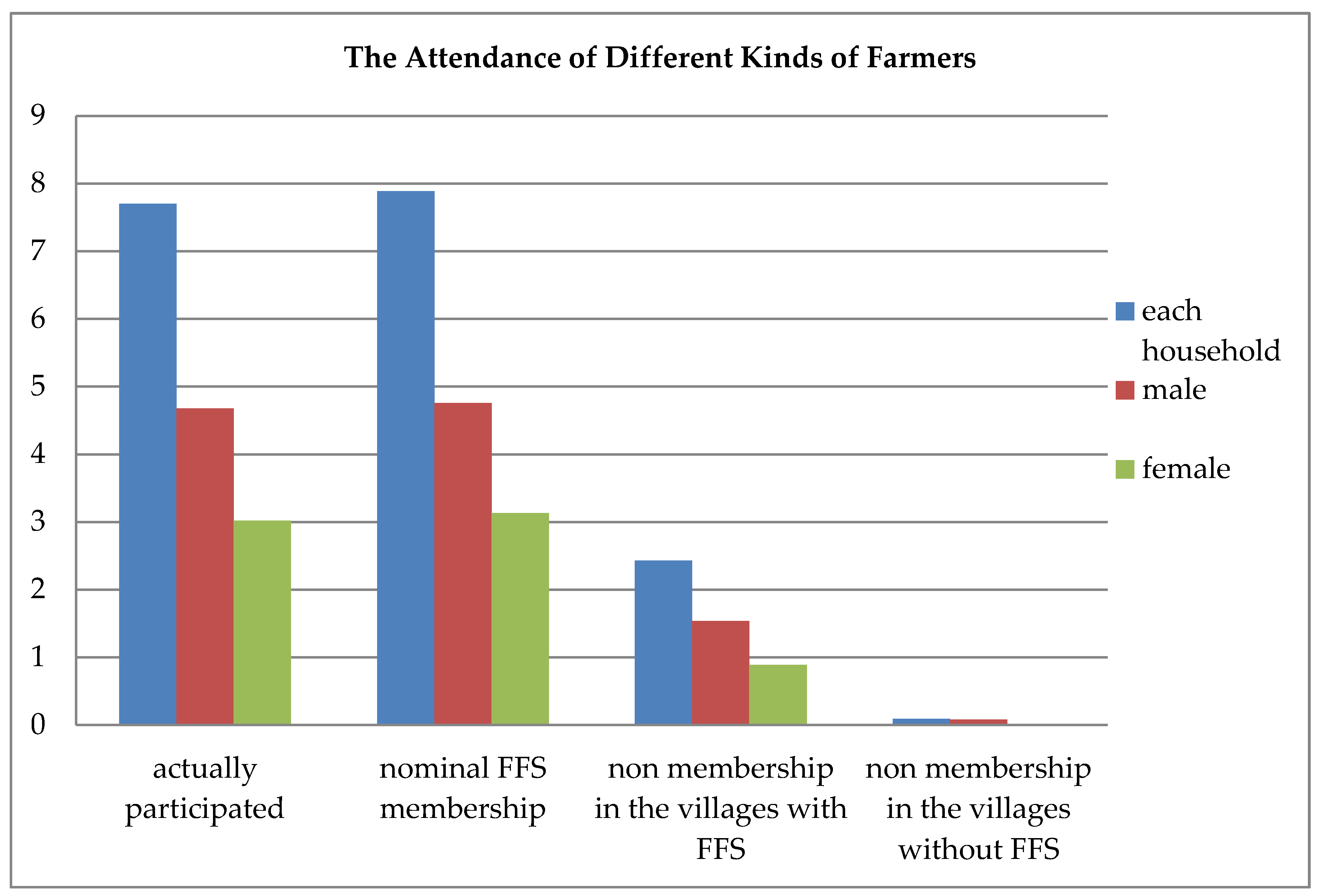
We separate the FFS farmers into three groups: (1) those with nominal FFS membership; (2) those without the nominal membership but living in a village with FFS offered; and (3) those living in a village without a FFS. Note that no villagers will have a nominal membership if there is no FFS offered in that village.

Figure 1 presents the FFS attendance rate by these three groups of farmers. For farmers who actually participated in the FFS training, on average, each household attends 7.7 sessions, of which the male member attends 4.68 sessions, and the female member attends the remainder. The attendance rate is approximately 55% (7.7/14). For all three groups, the attendance rates for male farmers are higher than those of the female farmers. The attendance rate of group (1) farmers is much higher than that of the other two groups: 56.4% (7.89/14) versus 17.4% (2.43/14) versus 0.6% (0.09/14). Although the attendance rate for group (3) farmers is very low, it may reflect the diffusion effect of FFS. Farmers in this group must be attracted to the training via word of mouth of their friends in the FFS villages.

Figure 1. The attendance of different kinds of farmers

Figure 1. The attendance of different kinds of farmers

7.2. The Determinants of Farmers’ Attendance in Farmer Field School

We pooled groups (1) and (2) in estimating Equation (7). Group (3) is excluded because there is no FFS in those villages and farmers may face different problems than those face by groups (1) and (2). The results from the zero-inflated Poisson model are presented in Table 6.

Table 6. Determinants of attendance in Farmer Field Schools.

Variables	(1) Probability of Having Zero Attendance_Man	(2) Man’s Attendance	(3) Probability of Having Zero Attendance_Woman	(4) Woman’s Attendance
household head	−2.052 ***	0.174	−2.290 ***	0.261 ***
	(0.411)	(0.139)	(0.408)	(0.090)
age_hus	−0.018	0.076 *	−0.548	0.225 *
	(0.258)	(0.042)	(0.408)	(0.116)
age square_hus	0.0008	−0.00075 *	0.005	−0.0019
	(0.0028)	(0.00043)	(0.004)	(0.0012)
education_hus	−0.001	0.093 ***	0.036	0.027
	(0.082)	(0.019)	(0.083)	(0.023)
farmtime_hus	−0.014 **	−0.0037 **	0.0066	−0.0039 **
	(0.0066)	(0.0016)	(0.0069)	(0.0017)
age_wife	0.927 ***	−0.098 **	−0.360	0.054
	(0.358)	(0.040)	(0.420)	(0.093)
age square_wife	−0.0106 ***	0.00088 **	0.004	−0.001
	(0.0039)	(0.0004)	(0.004)	(0.001)
education_wife	0.041	−0.035 ***	−0.033	−0.020
	(0.068)	(0.013)	(0.068)	(0.023)
farmtime_wife	−0.009	0.0068	−0.0045	−0.012
	(0.014)	(0.0046)	(0.016)	(0.011)
family size	−0.144	0.030	0.461 **	−0.052
	(0.163)	(0.031)	(0.180)	(0.049)
number of kids	0.960 *	−0.037	−0.705	0.241
	(0.522)	(0.115)	(0.540)	(0.149)
passets	−1.186	0.978 ***	3.719 *	0.176
	(1.631)	(0.320)	(1.953)	(0.640)
landsmall	1.033 ***	0.138 *	0.207	−0.037
	(0.333)	(0.075)	(0.337)	(0.091)
constant	−17.50 **	1.352	20.68 ***	−2.809
	(6.945)	(0.863)	(7.838)	(2.484)
observations	229	229	229	229

Note: Standard deviations reported in parentheses. ***, **, * indicate statistically significant at the 1%, 5% and 10%, respectively. Source: authors’ own survey.

Table 6. Determinants of attendance in Farmer Field Schools.

Variables	(1) Probability of Having Zero Attendance_Man	(2) Man’s Attendance	(3) Probability of Having Zero Attendance_Woman	(4) Woman’s Attendance
household head	−2.052 ***	0.174	−2.290 ***	0.261 ***
	(0.411)	(0.139)	(0.408)	(0.090)
age_hus	−0.018	0.076 *	−0.548	0.225 *
	(0.258)	(0.042)	(0.408)	(0.116)
age square_hus	0.0008	−0.00075 *	0.005	−0.0019
	(0.0028)	(0.00043)	(0.004)	(0.0012)
education_hus	−0.001	0.093 ***	0.036	0.027
	(0.082)	(0.019)	(0.083)	(0.023)
farmtime_hus	−0.014 **	−0.0037 **	0.0066	−0.0039 **
	(0.0066)	(0.0016)	(0.0069)	(0.0017)
age_wife	0.927 ***	−0.098 **	−0.360	0.054
	(0.358)	(0.040)	(0.420)	(0.093)
age square_wife	−0.0106 ***	0.00088 **	0.004	−0.001
	(0.0039)	(0.0004)	(0.004)	(0.001)
education_wife	0.041	−0.035 ***	−0.033	−0.020
	(0.068)	(0.013)	(0.068)	(0.023)
farmtime_wife	−0.009	0.0068	−0.0045	−0.012
	(0.014)	(0.0046)	(0.016)	(0.011)
family size	−0.144	0.030	0.461 **	−0.052
	(0.163)	(0.031)	(0.180)	(0.049)
number of kids	0.960 *	−0.037	−0.705	0.241
	(0.522)	(0.115)	(0.540)	(0.149)
passets	−1.186	0.978 ***	3.719 *	0.176
	(1.631)	(0.320)	(1.953)	(0.640)
landsmall	1.033 ***	0.138 *	0.207	−0.037
	(0.333)	(0.075)	(0.337)	(0.091)
constant	−17.50 **	1.352	20.68 ***	−2.809
	(6.945)	(0.863)	(7.838)	(2.484)
observations	229	229	229	229

Note: Standard deviations reported in parentheses. ***, **, * indicate statistically significant at the 1%, 5% and 10%, respectively. Source: authors’ own survey.

To capture the gender effects, we run the regression for males and females separately. The zero-inflated Poisson model is a combination of the logit model and the standard Poisson model. There are two sets of results: the first set shows the chances that a given independent variable affected the “structural” zeros; and the second set shows the results for the “sampling” counts [33]. Column (1) and column (2) in Table 6 show the first and second sets of results for male farmers, and column (3) and column (4) show the corresponding results for female farmers.

Both columns (1) and (3) in Table 6 suggest that being a household head has a positive effect on the decision to attend FFS. This is likely because the household head usually makes decisions regarding agricultural activities. The fraction of farming time of male farmers has a significant impact on whether or not the male farmer will attend the FFS training sessions. If the male farmer devotes more of his time to farming, he will be more likely to attend the FFS. The results in column (1) suggest that husbands with older wives are more likely to attend the FFS, but the probability increases at a decreasing rate and reverses when the wife’s age is more than 44 (0.927/(2 × 0.0106)) years old. One possible reason for this is that husbands with younger wives may assume more child bearing and care responsibilities. Thus, they are unable to go to the FFS. The results also show that more children in the family will have a negative impact on the male farmers’ participation in FFS. This is reasonable because more children will require more child care. The male farmers with land acreages below the sample average (at 0.33 hectare) are less likely to participate in FFS. However, once they decide to go, they will have more attendance compared with those with above average land size. Given that male farmer attendance has a positive impact on production, the results indicate that the FFS training is more beneficial for small land farmers. Results in column (2) show that male farmers with higher educational achievement and greater wealth but less land and less time devoted to farming attend more FFS sessions. Older male farmers attend more sessions, but at a decreasing rate. The peak is reached at age 51. Although male farmers with younger wives have a lower probability of attending, they show a tendency to attend more sessions once they decide to attend. Again, this trend will reverse when the wife’s reaches her mid-50s. The husband will attend more FFS sessions when his wife is less educated.

Column (3) presents the results of the female farmers’ probability of having zero attendance. In addition to the “household head” status effect as mentioned above, the larger and the wealthier the household, the less likely the woman will be to participate in the FFS. The results reported in column (4) suggest that the attendance of the female farmers will increase as their husbands get older. When the husband allocates more of his time to farming, the wife will attend fewer FFS sessions.

8. Conclusions and Policy Implications

Using data on FFS programs targeting tomato farmers in Beijing, this article finds that FFS participation significantly improves the production of tomato farmers. In contrast to Davis [18], our results suggest that the effect of FFS training is better for men than for women. Our results show that the attendance of male farmers in FFS has a significant impact on tomato yields, whereas the estimated coefficient of the FFS attendance is statistically insignificant for female farmers. This may be due to a lack of potential accumulation effects as female farmers attend fewer sessions and may not accumulate sufficient knowledge to have a positive impact on production.

Given the evidence we found on the potential positive impact of the FFS attendance, we examine the determinants of participation in FFS. The estimates show that farmers with less land are less likely to participate in the FFS; however, once they decide to participate, they will have greater attendance compared with farmers with larger amounts of land. This result indicates that the FFS training is more beneficial for small-scale farmers and hence may lead to recommendations for a conscious effort on the part of FFS to include farmers with smaller farms in the training process. Education and wealth are also significant determinants of male farmers’ attendance in FFS. Well educated male farmers from wealthier households are likely to have greater attendance. The fraction of farming time of male farmers has a positive impact on participation in FFS but has a negative impact on attendance. Age and educational achievement of male farmers seem to have substitute effects in determining their FFS attendance.

In light of the empirical results from this study, the FFS program should be expanded to more areas to benefit more farmers. Because the attendance of farmers has positive impact on their yield, actions should be taken (such as giving a small gift) to make the training more attractive and to encourage and ensure the participation of farmers. Since female farmers attend fewer sessions, actions also should be taken (such as help them with the baby sitting) to ensure their attendance. Compared with the small-scale farmers, the large-scale farmers are more likely to participate but attend fewer sessions, therefore actions should be also taken (such as make the attendance of large-scale farmers compulsory) to ensure their attendance. The FFS program should target small-size, well-educated and wealthier male farmers because the FFS program appeared to be more beneficial for them. Overall, the results discussed above imply that farmer field schools are a useful way to increase the production of farmers in Beijing.

References and Notes

- Kenmore, P.E. Indonesia’s Integrated Pest Management: A Model for Asia; Manila: FAO Inter-Country Programme for Integrated Pest Control in Rice in South and Southeast Asia: Manila, Pilipinas, 1991. [Google Scholar]
- Quizon, J.; Feder, G.; Murgai, R. Fiscal sustainability of agricultural extension: The case of the farmer field school approach. J. Int. Agric. Ext. Educ. 2001, 8, 13–24. [Google Scholar] [CrossRef]
- Feder, G.; Savastano, S. The role of opinion leaders in the diffusion of new knowledge: The case of integrated pest management. World Dev. 2006, 34, 1287–1300. [Google Scholar] [CrossRef] [Green Version]
- Anandajayasekeram, P.; Davis, K.E.; Workneh, S. Farmer field schools: An alternative to existing extension systems? Experience from Eastern and Southern Africa. J. Int. Agric. Ext. Educ. 2007, 14, 81–93. [Google Scholar] [CrossRef]
- Friis-Hansen, E.; Duveskog, D. The empowerment route to well-being: An analysis of farmer field schools in East Africa. World Dev. 2012, 40, 414–427. [Google Scholar] [CrossRef]
- Feder, G.; Murgai, R.; Quizon, J.B. The acquisition and diffusion of knowledge: The case of pest management training in farmer field schools, Indonesia. J. Agr. Econ. 2004, 55, 221–243. [Google Scholar] [CrossRef]
- Van den Berg, H.; Jiggins, J. Investing in farmers—the impacts of farmer field schools in relation to integrated pest management. World Dev. 2007, 35, 663–686. [Google Scholar] [CrossRef]
- Larsen, A.F.; Lilleør, H.B. Beyond the Field: The Impact of Farmer Field Schools on Food Security and Poverty Alleviation. World Dev. 2014, 64, 843–859. [Google Scholar] [CrossRef]
- Feder, G.; Murgai, R.; Quizon, J.B. Sending farmers back to school: The impact of farmer field schools in Indonesia. Appl. Econ. Perspect. Pol. 2004, 26, 45–62. [Google Scholar] [CrossRef]
- Simpson, B.M.; Owens, M. Farmer field schools and the future of agricultural extension in Africa. J. Int. Agric. Ext. Educ. 2002, 9, 29–36. [Google Scholar] [CrossRef]
- Tripp, R.; Wijeratne, M.; Piyadasa, V.H. What should we expect from farmer field schools? A Sri Lanka case study. World Dev. 2005, 33, 1705–1720. [Google Scholar] [CrossRef]
- Röling, N.; Van De Fliert, E. Transforming extension for sustainable agriculture: The case of integrated pest management in rice in Indonesia. Agric. Hum. Values 1994, 11, 96–108. [Google Scholar] [CrossRef]
- Kenmore, P. A perspective on IPM. ILEIA Newsl. 1997, 13, 8–9. [Google Scholar]
- Godtland, E.M.; Sadoulet, E.; de Janvry, A.; Murgai, R.; Ortiz, O. The impact of farmer field schools on knowledge and productivity: A study of potato farmers in the Peruvian Andes. Econ. Dev. Cult. Chang. 2004, 53, 63–92. [Google Scholar] [CrossRef]
- Palis, F.G. The role of culture in farmer learning and technology adoption: A case study of farmer field schools among rice farmers in central Luzon, Philippines. Agric. Hum. Values 2006, 23, 491–500. [Google Scholar] [CrossRef]
- Mauceri, M.; Alwang, J.; Norton, G.; Barrera, V. Effectiveness of integrated pest management dissemination techniques: A case study of potato farmers in Carchi, Ecuador. J. Agric. Appl. Econ. 2007, 39, 765–780. [Google Scholar]
- Bartlett, A. Farmer Field Schools to Promote Integrated Pest Management in Asia: the FAO Experience. In Proceedings of Workshop on Scaling Up Case Studies in Agriculture, Bangkok, Thailand, 16–18 August 2005.
- Davis, K.; Nkonya, E.; Kato, E.; Mekonnen, D.A.; Odendo, M.; Miiro, R.; Nkuba, J. Impact of farmer field schools on agricultural productivity and poverty in East Africa. World Dev. 2012, 40, 402–413. [Google Scholar] [CrossRef]
- Yorobe, J.; Rejesus, R.; Hammig, M. Insecticide use impacts of integrated pest management (IPM) farmer field schools: Evidence from onion farmers in the Philippines. Agric. Syst. 2011, 104, 580–587. [Google Scholar] [CrossRef]
- Yang, P.; Liu, W.; Shan, X.; Li, P.; Zhou, J.; Lu, J.; Li, Y. Effects of training on acquisition of pest management knowledge and skills by small vegetable farmers. Crop Protect. 2008, 27, 1504–1510. [Google Scholar] [CrossRef]
- It is difficult to tell in which year the program was discontinued because except for the FFS in Beijing, other FFSs are carried out as a “program”. More than 92% of the FFS programs in China are supported by the FAO. The FFS programs usually last for one or two years in one place. Then the FAO will set up other FFS programs in other provinces. When the program is over, the FFSs are discontinued. During the 1990s, FAO supported many FFSs in China. By 1997, 21 provinces had set up FFSs, and then FAO cut their funding. The most recent FFS programs that we can find are (1) the BT cotton FFS supported by the EU & FAO in 2000–2004 in five provinces, and (2) a vegetable FFS supported by the FAO in Yunnan province from 2005–2007.
- Wuepper, D.; Sauer, J.; Kleemann, L. Sustainable Intensification of Pineapple Farming in Ghana: Training and Complexity. Available online: https://www.econstor.eu/dspace/bitstream/10419/103980/1/805019839.pdf (accessed on 29 January 2016).
- Böhning, D.; Dietz, E.; Schlattmann, P.; Mendonca, L.; Kirchner, U. The zero-inflated Poisson model and the decayed, missing and filled teeth index in dental epidemiology. J. R. Stat. Soc. A Stat. Soc. 1999, 162, 195–209. [Google Scholar] [CrossRef]
- Jansakul, N.; Hinde, J. Score tests for zero-inflated Poisson models. Comput. Stat. Data Anal. 2002, 40, 75–96. [Google Scholar] [CrossRef]
- Yang, Z.; Hardin, J.W.; Addy, C.L. Testing overdispersion in the zero-inflated Poisson model. J. Stat. Plan. Inference 2009, 139, 3340–3353. [Google Scholar] [CrossRef]
- Wooldridge, J. Introductory Econometrics: A Modern Approach; Thomson Learning: New York, NY, USA, 2003; pp. 595–600. [Google Scholar]
- Cox, D.R. Some remarks on overdispersion. Biometrika 1983, 70, 269–274. [Google Scholar] [CrossRef]
- Dean, C.; Lawless, J.F. Tests for detecting overdispersion in Poisson regression models. J. Am. Stat. Assoc. 1989, 84, 467–472. [Google Scholar] [CrossRef]
- Gurmu, S.; Trivedi, P.K. Excess zeros in count models for recreational trips. J. Bus. Econ. Stat. 1996, 14, 469–477. [Google Scholar]
- Miaou, S.-P. The relationship between truck accidents and geometric design of road sections: Poisson versus negative binomial regressions. Accid. Anal. Prev. 1994, 26, 471–482. [Google Scholar] [CrossRef]
- Wedderburn, R.W. Quasi-likelihood functions, generalized linear models, and the Gauss—Newton method. Biometrika 1974, 61, 439–447. [Google Scholar]
- Jang, H.; Lee, S.; Kim, S.W. Bayesian analysis for zero-inflated regression models with the power prior: Applications to road safety countermeasures. Accid. Anal. Prev. 2010, 42, 540–547. [Google Scholar] [CrossRef] [PubMed]
- Hu, M.-C.; Pavlicova, M.; Nunes, E.V. Zero-inflated and hurdle models of count data with extra zeros: examples from an HIV-risk reduction intervention trial. Am. J. Drug Alcohol Abuse 2011, 37, 367–375. [Google Scholar] [CrossRef] [PubMed]
- Lambert, D. Zero-Inflated Poisson Regression, with an Application to Defects in Manufacturing. Technometrics 1992, 34, 1–14. [Google Scholar] [CrossRef]
© 2016 by the authors; licensee MDPI, Basel, Switzerland. This article is an open access article distributed under the terms and conditions of the Creative Commons by Attribution (CC-BY) license (http://creativecommons.org/licenses/by/4.0/).
Share and Cite
MDPI and ACS Style
Cai, J.; Shi, G.; Hu, R. An Impact Analysis of Farmer Field School in China. Sustainability 2016, 8, 137. https://doi.org/10.3390/su8020137
AMA Style
Cai J, Shi G, Hu R. An Impact Analysis of Farmer Field School in China. Sustainability. 2016; 8(2):137. https://doi.org/10.3390/su8020137
Chicago/Turabian StyleCai, Jinyang, Guanming Shi, and Ruifa Hu. 2016. "An Impact Analysis of Farmer Field School in China" Sustainability 8, no. 2: 137. https://doi.org/10.3390/su8020137
Note that from the first issue of 2016, this journal uses article numbers instead of page numbers. See further details here.