Article

Wave Climate Resource Analysis Based on a Revised Gamma Spectrum for Wave Energy Conversion Technology

1
Department of Mechanical Engineering, University of Louisiana at Lafayette, Lafayette, LA 70504, USA
2
Department of Mechanical Engineering, Mississippi State University, Mississippi State, MS 39760, USA
*
Author to whom correspondence should be addressed.
Sustainability 2016, 8(12), 1321; https://doi.org/10.3390/su8121321
Submission received: 11 October 2016 / Revised: 24 November 2016 / Accepted: 8 December 2016 / Published: 14 December 2016
(This article belongs to the Special Issue Wave Energy Converters)

Abstract

:
In order to correctly predict and evaluate the response of wave energy converters (WECs), an accurate representation of wave climate resource is crucial. This paper gives an overview of wave resource modeling techniques and applies a methodology to estimate the naturally available and technically recoverable resource in a given deployment site. The methodology was initially developed by the Electric Power Research Institute (EPRI), which uses a modified gamma spectrum to interpret sea state hindcast parameter data produced by National Oceanic and Atmospheric Administration’s (NOAA’s) WaveWatch III. This gamma spectrum is dependent on the calibration of two variables relating to the spectral width parameter and spectral peakedness parameter. In this study, this methodology was revised by the authors to increase its accuracy in formulating wavelength. The revised methodology shows how to assess a given geographic area’s wave resource based on its wave power density and total annual wave energy flux.

1. Introduction

This paper presents a systematic methodology to parameterize the wave energy resource for a given deployment site where a wave energy converter (WEC) is applied. The presented methodology allows us to evaluate the WEC’s response and power product for a finite rage of values on significant wave height (Hs), and the peak wave period (Tp). Based on the calculated WEC’s response and power production at one site, the WEC’s performance at other sites with different sea states can be estimated through a numerical interpolation [1,2]. At present, a power matrix in terms of Hs, Tp, or energy period (Te) is being used by WEC developers employed to represent a WEC’s output power. However, due to the fact that there exist different spectral shapes for a given Hs and Tp, the same power matrix may result in a variety of estimations in the power produced by the WEC, which leads to significant error [3].
In order to eliminate the barrier caused by the limited descriptive ability of the power matrix, the Department of Trade and Industry (DTI) in the United Kingdom (U.K.) presented a preliminary wave energy device performance protocol, which describes the response of a WEC through several tables that outline the mean, standard deviation, and minimum and maximum power for each cell of the power matrix [4]. This technique is relatively simple to use; nevertheless, the distribution of spectral shapes for a given Hs and Tp is highly dependent on the deployment location of the WECs. Therefore, for each potential deployment site of WECs, such a table has to be created to depict the distribution of spectral shapes for the Hs and Tp in that location. This type of work can be very laborious and time consuming if a number of sites are selected for deploying the WEC.
Smith et al. used a variety of bandwidth parameters to define the spread in energy within the sea state. Correlations between the sea bandwidth parameters and the width of power transfer functions were identified, and the effect of two generic power transfer functions on power production from six simulated wave spectra were examined [5]. Fusco et al. presented a methodology to assess the possible benefits of the combination of wind energy with the wave energy through analysis of the raw wind and wave resource at certain locations around the coasts of Ireland [6]. In that study, a wave system was also defined by Hs and Tp. Folley and Whittaker used a third-generation spectral wave model to model the wave transformation from deepwater to a nearshore site in a water depth of 10 m. The wave transformation model was then employed to calculate a site’s potential using the exploitable wave energy resource [7]. Carballo and Iglesias extracted significant wave height, energy period, and mean wave direction and characterized the wave resource based on the probability distribution of the three parameters using a Joint North Sea Wave Observation Project (JONSWAP) spectrum. Power performance that can be obtained at a location of interest with a certain WEC technology was then determined based on the various wave cases, both on a monthly and annual basis [8].
Duclos et al. [9] showed that optimizing the WEC necessitates accounting for all possible wave conditions weighted by their annual occurrence frequency, as generally given by the classical wave climate scatter diagrams. A generic and simple wave energy converter was also presented to show how the optimal parameters depend on the very different wave climates. Besides that, the influence of the wave climate on the design and annual production of electricity by oscillating water column (OWC) wave power plants was also investigated by Sarmento et al. [10].
Based on the current progress made in wave resource description and WEC power response evaluation, this paper will continue to review different models for omnidirectional wave spectra and then outline and revise a systematic methodology to estimate two quantities for characterizing the naturally available wave energy resource in a given area, as given by the Electric Power Research Institute (EPRI) [11]. The EPRI method is based on a calibration of spectral width parameter, n, which is observed to have a significant influence on the wave power density and is proved to be robust in all ocean regions evaluated, including the North Pacific Ocean, Gulf of Mexico, and the Caribbean Sea. The remaining sections of this paper are organized as follows: Section 2 describes the standard spectral models; Section 3 presents a five-step technical approach for estimating the wave energy resource, the wave power density values, and the annual wave energy flux in a given region; Section 4 presents a case study to apply this method to estimate the available wave energy for a localized geographic location and validate the results by comparing to current data; the entire paper is concluded by Section 5.

2. Omnidirectional Wave Spectral Models

Equation (1) [12] gives a family of equations which are most commonly used for assessing the unimodal spectra:
S ( f ) = α f r e x p ( β f s ) γ a ( f )
Here α, β, r, s > 0, and γ ≥ 1, and
a ( f ) = e x p ( 1 2 ( f f p σ f p ) 2 )
σ = { 0.07   f o r   f < f p 0.09   f o r   f f p
where fp is the peak frequency of the spectrum and defined as
f p = ( s β / r ) 1 / s
In Equation (1), α and β are scale and shift parameters, which depend on Hs and Tp, r and s are parameters that control the shape of the spectrum, γ is the peak enhancement factor, and a(f) is the peak intensity function. Overall, five free parameters are needed to fully define the family of spectra (Equations (1)–(4)). In order to reduce the number of free variables in describing the sea state, some parameters can be fixed with constant values while the remaining parameters still stay free. Thus, one can obtain different forms originally converted from Equation (1).
For example, the classic Bretschneider form [10] was converted from Equation (1) by taking r = 5, s = 4, and γ = 1. Pierson and Moskowitz proposed a special form of the Bretschneider spectrum for fully developed seas in the Northern Atlantic Ocean generated by local winds [13]. In the Pierson–Moskowitz spectrum, α is a function of wind speed, and the energy in the spectrum depends on the value of β only. Hasselmann et al. modified the Pierson–Moskowitz spectrum by enforcing that γ ≠ 1, in order to improve the fit to the more peaked spectral shapes observed in the fetch-limited wind seas during the Joint North Sea Wave Observation Project (JONSWAP) [14]. Based on the fundamental Bretschneider, Pierson–Moskowitz, and JONSWAP spectra, Ochi and Hubble proposed a wave spectrum, which is the sum of two separate component spectra in order to represent sea states that include both remotely generated swell and local wind-generated sea [15]. The Ochi–Hubble spectrum suggested that s = 4 and γ = 1, leaving r a free parameter; a gamma-type spectrum was used in that spectrum to describe the swell component of the two-peaked spectrum. Lately, Boukhanovsky and Soares extended that gamma-type spectrum to present a gamma spectrum that approximates any frequency spectrum with γ = 1 and s = (r − 1) and used that spectrum to model the multipeaked directional wave spectra [16].
Boukhanovsky’s research showed the advantage of the proposed gamma spectrum in modeling multipeaked directional wave spectra, which occur with a high percentage in the location of interest of this study. Moreover, the reliability of the gamma spectrum in wave spectra modeling and reconstruction was also verified through employing it to model ocean conditions in the Gulf of Mexico [17,18]. Therefore, in this paper, the use of the gamma spectra will be modified to include two spectral shape coefficients. The calibration objective is to find values of these coefficients for a given region through an iterative process in order to reconstruct the overall sea state spectra that would best fit the full hindcast spectra for the given region of a selected deepwater calibration station.

3. Methodology for Estimating the Available Wave Energy Resource

In a recent study conducted by the EPRI, data was collected from U.S. coastal waters for a 51-month WaveWatch III hindcast database that was developed specifically for the EPRI by the National Center for Environmental Prediction (NCEP) of National Oceanic and Atmospheric Administration (NOAA) [19]. The EPRI’s method was validated by comparing the WaveWatch III hindcast results with the wave measurements recorded during the same time period. According to this methodology, two quantities will be found and estimated for characterizing the naturally available wave energy resource in a given site. Those two quantities are the wave power density (kilowatt per meter of wave crest width) and the total annual wave energy flux (TW-h per year). Five major steps need to be followed to obtain these two quantities. A flowchart showing this five-step method is plotted in Figure 1.

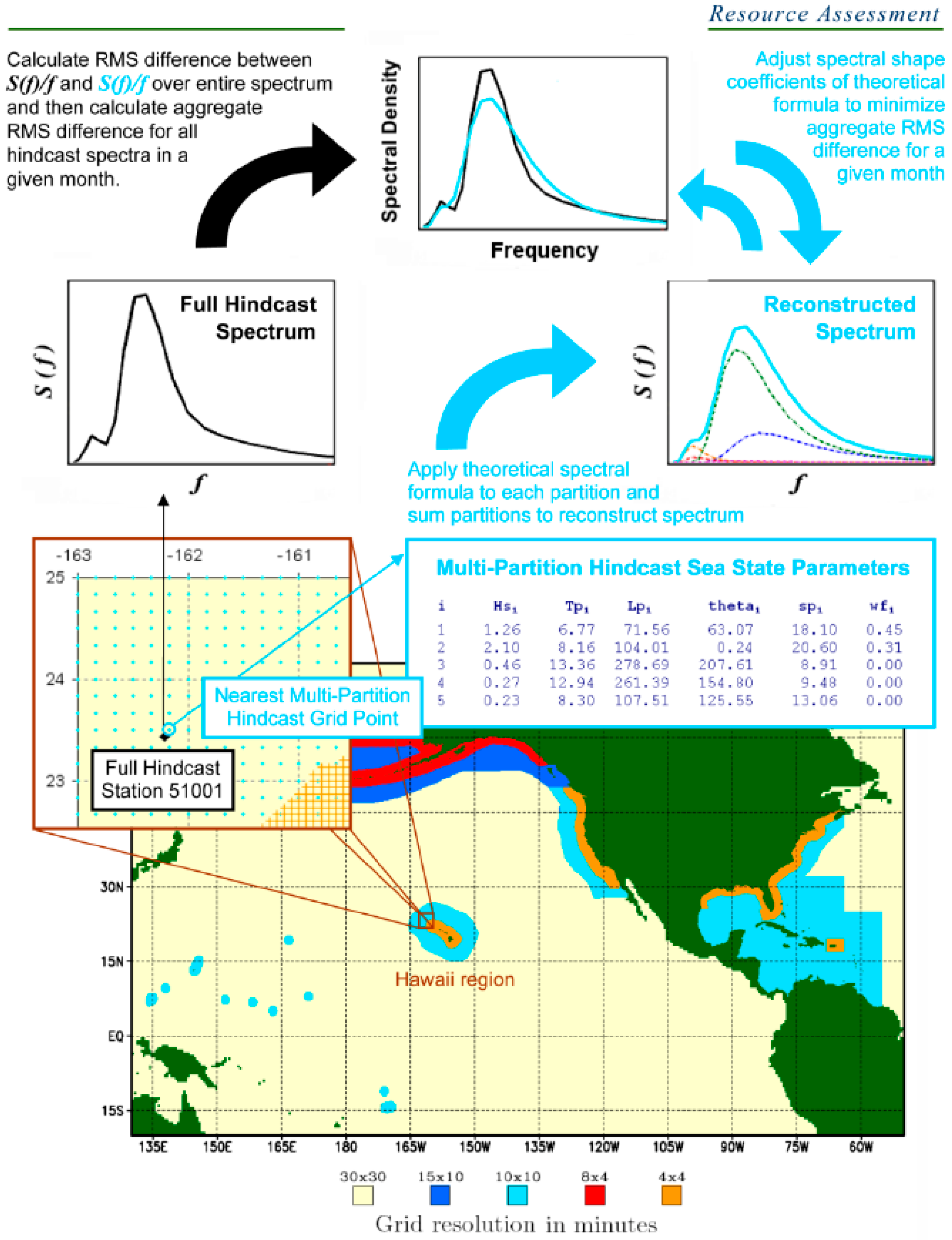
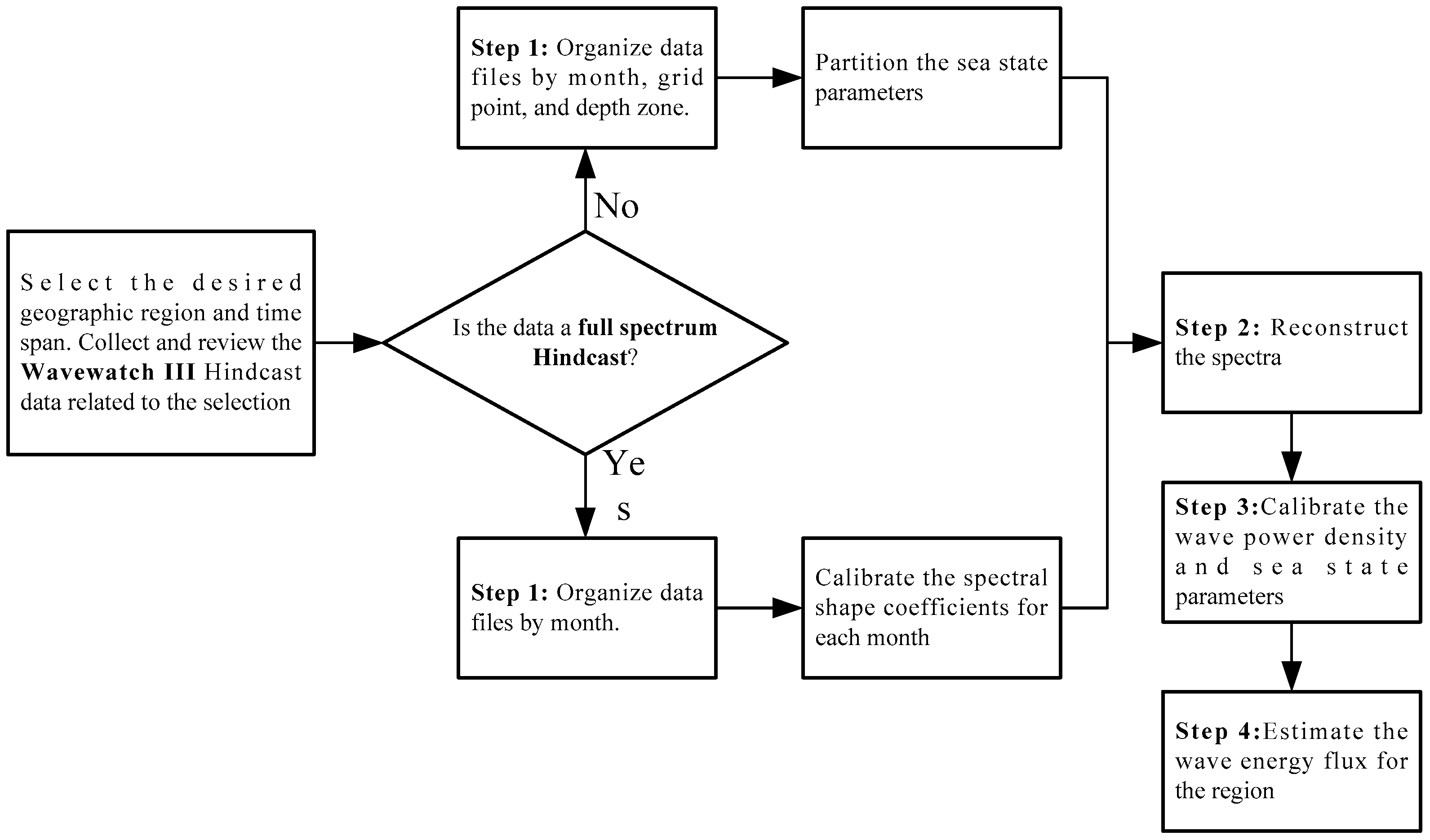
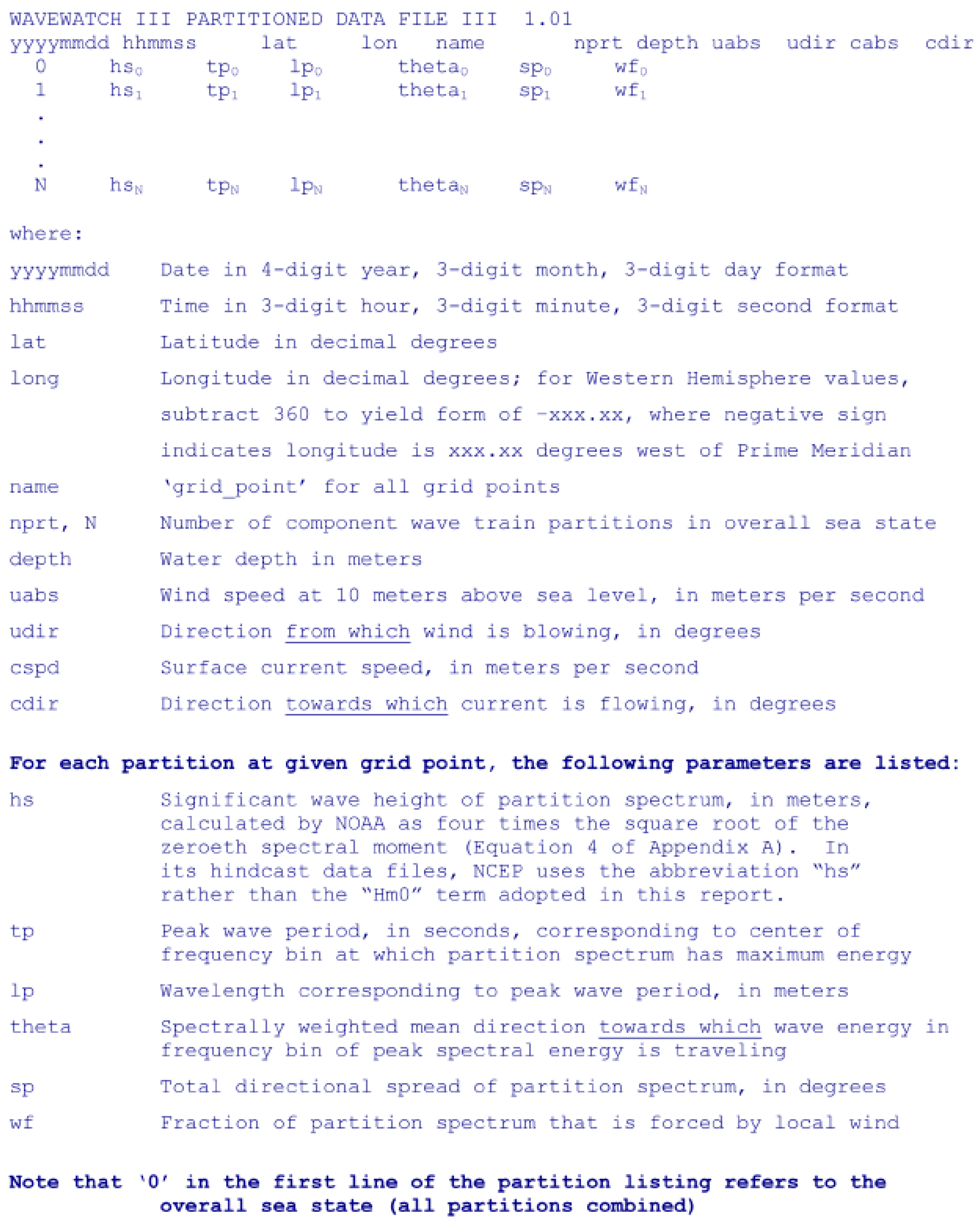
3.1. Preprocess WaveWatch III Multi-Partition Hindcast of Sea State Parameters

In step 1, the large gridded hindcast data files produced by NCEP are preprocessed and converted into a more usable and accessible database structure. WaveWatch III solves the random-phase spectral action density balance equation for wavenumber–direction spectra. In this equation, it is assumed that properties of the medium (water depth and current) as well as the wave field itself vary on time and space scales that are much larger than the variation scales of a single wave. The raw data (grid points) given from the WaveWatch database are the full directional spectrum data (in frequency domain), which need to be first converted to the nondirectional data (in time domain) and organized into its time slot. The conversions will be performed by the WaveWatch III model at 3 h intervals for all grid points. Due to the fact that the full directional spectrum contains such a vast amount of information (24 directions × 25 frequency bins = 600 values per hindcast), the full directional spectrum is only achieved for 275 grid points around the world. If a full directional spectrum is available, then these values need to be converted into the nondirectional wave spectrum.

3.1.1. Calculating Nondirectional Spectrum from Directional Spectrum

The term “nondirectional spectrum” here is referred as the “nondirectional wind wave sea surface elevation variance density spectrum”, which is the integral of the directional wave spectrum over all directions (dθ) at each frequency. Therefore, given S(f, θ) as the directional wave spectrum in m2/Hz/radians, then the nondirectional wave spectrum S(f) is in m2/Hz and can be calculated as follows:
S ( f ) = 0 2 π S ( f , θ ) d θ = Δ θ i = 1 N d S ( f , θ i ) = 2 π N i = 1 N d S ( f , θ i )
where Nd is the number of directional bins, which is 24 in the WaveWatch III model; θ is the wave direction in radians; and f is the frequency in Hz. Now that the nondirectional wave spectrum is established, the spectral moments can equally be computed directly from the directional spectrum.

3.1.2. Calculating the Spectral Moments from the Nondirectional Spectrum

In order to calibrate the spectral shape coefficients and calculate the sea state parameters from the nondirectional wave spectrum, the nth spectral moment needs to be defined as:
m n = 0 f n S ( f ) d f = i = 1 N f ( f i ) n S ( f i ) Δ f i
where Nf is the number of frequency bins, which is 25 for the WaveWatch III database, and Δfi is the frequency bin width for the ith bin.
In order to establish an iterative process, two initial spectral moments m0 and m−1, are defined as:
m 0 = i = 1 N S ( f i ) Δ f i
m 1 = i = 1 N S ( f i ) f i Δ f i
These moments are required for calculating the significant wave height, wave energy period, and wave power density.
The remaining grid points only include three sea state parameters: spectrally derived significant wave height (Hm0), peak wave period (Tp), and mean direction of spectral peak energy (θp). Though such a database of fully partitioned sea state parameters does not provide as much information as contained in the full directional spectrum, the information is sufficient enough to reconstruct the nondirectional spectrum by applying a theoretical spectral formulation to each partition, and then summing the remaining spectra across all partitions or component wave trains. This will be completed in step 2. Before that, the large gridded hindcast data files produced by the NCEP need to be preprocessed into a more usable and accessible database structure.

3.1.3. Organizing the Directional Data

After obtaining the nondirectional data, those data have to be sorted and organized into a database structure. In order to do that, the grid points for specific geographic area and mapping limitations will be selected, and the selected points will then be organized into a file structure that has all the time steps for a given month as an individual file for each grid point.
The WaveWatch III hindcast file produced by NCEP is structured monthly. The multi-partition sea state parameter values are assigned to every grid point throughout a given geographic domain of the file at a particular time step, and those values are updated for each grid point for the next time step. The interval between two neighboring time steps is 3 h. Typically, the large gridded domains have a spacing of 4 min in longitude and latitude. In preprocessing the data, only the grid points for the specific geographic area and mapping limitations will be selected and organized into a file structure that has all the time steps for given months, in which an individual file is created for each grid point. An example of the organized data structure is displayed in the Appendix A, which shows a sorting of files by region, depth zone, grid point, and month.

3.2. Calibrate the Spectral Shape Coefficients

From the given sea state parameters, the wave power density needs to be accurately calculated. In the present methodology, a modified gamma spectrum will be reconstructed and applied to each sea state partition. This modified gamma spectrum has two spectral shape coefficients. In order to find these coefficients, a calibration process needs to be performed to find their values for a given region so as to reconstruct the overall sea state spectra that would best fit the full hindcast spectra for that region from a selected deepwater calibration station.
It can be observed that the wave power density is directly proportional to m−1 of the wave spectrum (Equation (28)). The calibration technique developed by EPRI attempts to minimize the difference between the reconstructed spectrum and the full spectrum for S(f)/f, which is the integrand of m−1 (Equation (28)). The root-mean-square (RMS) difference in S(f)/f between the reconstructed spectrum and the full hindcast spectrum over the entire range of frequencies for a particular time step will be first calculated. The RMS differences will then be aggregated over all time steps in a given month–year combination. Next, the shape coefficient (kb) value that leads to the least aggregate RMS difference can be found. Section 3.2.1 explains the formula for finding the wave spectrum, and Section 3.2.2 introduces how to calibrate the coefficients n and γ that are used for the formula presented in Section 3.2.1. The procedure for minimizing the RMS to get kb is basically the process of calibrating the coefficient n, which will be demonstrated in Section 3.2.2.
This procedure is demonstrated through the following equations.

3.2.1. Theoretical Gamma Spectral Formulation

The spectral formulation for a single wave train or partition developed by EPRI is derived from the basic gamma (Γ) spectrum equation [15,16] as:
S Γ ( f ) = A f n e x p [ B f ( n 1 ) ] γ a
where
A = n H m 0 2 T p 4
B = n T p 4
In these equations, n is the spectral width parameter and γ is the spectral peakedness parameter. The exponent parameter, a, defines the asymmetry around the spectral peak and is a function of f according to the following formula:
a = e x p [ ( f f p ) 2 σ 2 f p 2 ]
where σ is defined in Equation (3).
The gamma spectrum becomes the Bretschneider spectrum when n = 5 and γ = 1, whose shape depends only on two sea state parameters, Hm0 and Tp. The gamma spectrum becomes the JONSWAP spectrum when n = 5 and γ > 1, which has a peak overshoot characteristic for developing seas. Following Boukhanovsky and Soares’ approach [16], a full spectrum can be reconstructed as the sum of gamma spectra by calibrating either n or γ.

3.2.2. Calibrating n and γ for Use in the Gamma Spectra

Within any given hindcast partition there are two types of wave trains that can be represented by the shape factors n and γ. The type I sea state refers to the developing wind seas, so we set n = 5 and calibrate γ using Equation (12) to define the spectral peak asymmetry. The type II sea state refers to all other sea states (swells, decaying wind seas, and fully developed wind seas). For this type we set γ = 1 and calibrate the spectral width parameter, n.
The type I sea state is defined for the developing wind seas, and in order for such seas to develop the spectrum, the actual wave period needs to be longer than the peak period, Tp. This is due to the fact that waves characterized by shorter periods have already reached the steepness required for equilibrium and cannot grow higher without destabilizing or breaking. Within the spectra there exists a long-period cutoff, above which the wave energy in the spectra is traveling faster than the wind. This is because the wave group velocity is directly proportional to the angular frequency as cG = ∂w∂k, where k is the wavenumber. As long as the spectral peak period is less than the long-period cutoff, the spectrum can still develop further.
Another advantage of the WaveWatch III hindcast data is that it also produces local wind speed along with the sea state parameters. This advantage allows us to estimate the long-period cutoff using the Pierson–Moskowitz relationship [13]. This relationship can be used to identify the developing seas in the hindcast partitions. The Pierson–Moskowitz theoretical peak period for a fully developed sea state in complete equilibrium with the local wind speed, however, it can be used as the long-period cutoff. There is an inconsistency due to the fact that the wind speed in the Pierson–Moskowitz relationship is given at an elevation of 19.5 m above sea level and the WaveWatch III hindcast wind speed data is given at 10 m above sea level. In order to apply the Pierson–Moskowitz relationship for the WaveWatch III hindcast data, a 1/7-power law for the shear profile in the marine boundary is employed [19,20,21]. The peak wave period for fully developed seas, TpFD, can be calculated as:
T p F D = 2 π U 10 ( 1.95 ) ( 1 7 ) 0.87 g =   7.9450 U 10 g = 0.81016 U 10
where U10 is the WaveWatch III hindcast wind speed at 10 m above sea level and g is the gravitational acceleration, which is 9.81 m/s2.
Once TpFD is found, then it can be compared to the WaveWatch III hindcast peak period (Tp) for that given partition. If Tp < TpFD, then that partition is considered to be in a developing wind sea state and can be labeled as a type I sea state and calibrated accordingly, as stated above. If Tp > TpFD, then the partition is labeled as a type II sea state and n needs to be determined as:
n = 5 w f + k b T p ( 1 w f )
In Equation (14), Tp is the WaveWatch III hindcast peak period of the partition and wf is the hindcast wind fraction of the partition, which refers to the fraction of energy in a given partition forced by local winds. Note that the calibrated value of kb, as discussed above, is now implemented as a dimensional constant which models the dependency of the spectral width on the peak.
From Equation (14), if wf = 1, then n is calculated as 5, and the spectrum becomes the Bretschneider spectrum, which is appropriate for seas under the influence of local winds with no swell energy present. It was found by EPRI that kb indicates the spectral width of wave energy that is not influenced by the local winds [11]. It is the value of kb that is calibrated, which in turn determines n from Equation (14).

3.3. Reconstructing the Overall Spectra

In this step, the overall spectra can be reconstructed using the spectral shape parameters calibrated in previous steps, as Equation (9). By using the two data inputs (the hindcast sea state parameter data and the spectral shape coefficient data) for each partition in the given region, the spectra and the sea state parameters can be calculated in step 4 for each time step in a given month. If the time period of interest is 12 months, then there would be approximately 2920 hindcast time steps (the time interval is 3 h) on each grid point. The overall number of reconstructed overall sea state spectra during a 12-month period will then be equal to 2920 times the number of grid points in the region of interest. This reconstruction process is depicted in Figure 2.

3.4. Calculate Overall Sea State Parameters and Wave Power Density

In order to reconstruct the overall sea state spectrum, three parameters have to be decided, which consist of the significant wave height, the wave energy period, and the wave power density.
The first value is the spectrally derived significant wave height (Hm0), which can be calculated as:
H m 0 = 4 m 0
This value approximates time-series-derived significant wave height, which is the average of the highest third of the waves in a random seaway and generally corresponds to the mean wave height that could be estimated by visual observation due to the fact that the smaller waves can pass undetected by the human eyes. This figure was calculated and archived by WaveWatch III and can be found from [19].
The wave energy period (Te) can be determined from the two spectral moments (m−1 and m0), calculated above, as:
T e = m 1 m 0
The wave energy period Te is a sea state parameter that is not needed for further calculations, therefore, it is not archived in WaveWatch III. Usually, Te is estimated from other variables (such as Tp) when the spectral shape is unknown. For example, in preparing the Atlas of UK Marine Renewable Energy Resources, it was assumed that Te = 1.14Tz [22]. Alternatively, it can be estimated based on Tp as:
Te = αTp
The coefficient α depends on the shape of the wave spectrum: α = 0.86 for a Pierson–Moskowitz spectrum, and α increases towards unity with decreasing spectral width. In assessing the wave energy resource in southern New England, Hagerman [23] assumed that Te = Tp. In this study, we adopted the more conservative assumption of α = 0.90 or Te = 0.9Tp, which is equivalent to assuming a standard JONSWAP spectrum with a peak enhancement factor of γ = 3.3. It is readily acknowledged that this necessary assumption introduces some uncertainty into the resulting wave power estimates, particularly when the real sea state is comprised of multiple wave systems. However, since (in deepwater conditions) the wave power density, P, is proportional to Te(Hs)2, errors in period are less significant than errors in wave height. Also, this relation (Equation (17)) depends not only on the sea state (wave systems) in a particular location, but on the average sea state over all locations. The coefficient α may also change significantly from one location to another (precisely depending on the typical wave systems in those locations).
The peak wave period (Tp) is the inverse of the frequency at which the wave spectrum has its highest energy density, and is also referred to as the dominant wave period. This parameter is necessary for formulating the theoretical spectrum and is archived by WaveWatch III.
The mean direction of spectral peak energy (θp) is the spectrally weighted mean direction of the wave energy contained within the frequency bin that contains the peak wave period, Tp. This direction is measured using meteorological convention in degrees, and all directions are per compass rose (measured clockwise from north, with north staying at 0° and east 90°). This parameter is also archived by WaveWatch III.
The potential energy content (E) of a wave per unit area of water surface (J/m2) in an irregular sea state can be found as:
E = ρ g 0 S ( f ) d f = ρ g m 0 = ρ g H m 0 2 16
where g denotes the acceleration due to gravity. The potential energy should be equal to the kinetic energy; therefore, the total energy can be represented as 2E.
For each harmonic component of the wave spectrum, its energy travels at the group velocity (cG) as:
c G ( f , d ) = 1 2 g k tanh ( k d ) ( 1 + 2 k d sinh ( 2 k d ) )
where d is the water depth, and k is the wavenumber which is given by the dispersion relation:
( 2 π f ) 2 = ( 2 π T ) 2 = g k tanh ( k d )
where k = (2π)/L and L is the wavelength. In deepwater, where the local depth is greater than half a wavelength, tanh(kd) ≈ 1, and the dispersion relation can be simplified as:
( 2 π T ) 2 = g k
so that:
L 0 = g T 2 2 π
where the subscript “0” denotes deepwater. Therefore, the deepwater group velocity can be approximated as:
c G 0 = c 2 = L 0 2 T 0 = g T 4 π
In an effort to increase the accuracy of the current EPRI method, a formulation was found through the US Army Corps of Engineer’s Coastal Engineering Technical Note entitled “Direct methods for calculating wavelength” [24]. In our revised methodology, Equations (22) and (23) are replaced by Equations (24)–(26), which were proved to be more accurate. Equations (24)–(26) can be derived using Hunt’s method based on the Pade’s approximation [25], which are accurate to 0.1% for determining the wavelength in any depth of water [24]. It is noticed that there is no subscript “0” in Equation (24), and this is because that equation can be used for both deep and shallow water.
L = T g d F
F = G + 1 1 + 0.6522 G + 0.4622 G 2 + 0.0864 G 4 + 0.0675 G 5
G = ( 2 π T ) 2 d g
where F and G are known as the Pade’s approximation [25]. Alternatively, the wavelength can also be estimated using the Fenton formula [26], which is easier than above equations.
The wave power density (P), which is also referred to as the “wave energy flux”, is given in W/m of wave crest width at any given water depth, and is calculated as:
P = ρ g 0 c G ( f , d ) × S ( f ) d f = ρ g 2 4 π 0 S ( f ) f [ ( 1 + 2 k f d sinh ( 2 k f d ) ) tanh ( k f d ) ] d f
In deepwater, the term ( 1 + 2 k f d sinh ( 2 k f d ) ) tanh ( k f d ) → 1, therefore, the above equation is simplified to:
P 0 = ρ g 2 4 π m 1 = ρ g 2 64 π T e ( H m o ) 2 = 490 T e ( H m 0 ) 2
From the above equation, it is apparent that the wave power density is directly proportional to m-1 of the wave spectrum. In Equation (28), the seawater density ρ is 1025 kg/m3. Equation (27) shows that the calculation of the wave power density always involves the integration of S(f)/f multiplied by a depth (d)- and frequency (f)-dependent dispersion system. Thus, the overall spectrum has to be reconstructed before the wave power density can be determined.

3.5. Estimating the Total Wave Energy along a Depth Contour

In the last step, the total annual wave energy flux (TW-h/year) will be estimated based on the calculated wave power density for a given area. Usually a given region involves more than one depth contour, such as a region that incorporates deepwater to its nearest shore line. In that case, the estimation results should reflect how the decreasing depth affects the wave energy flux as the deepwater waves travel towards the shore line.

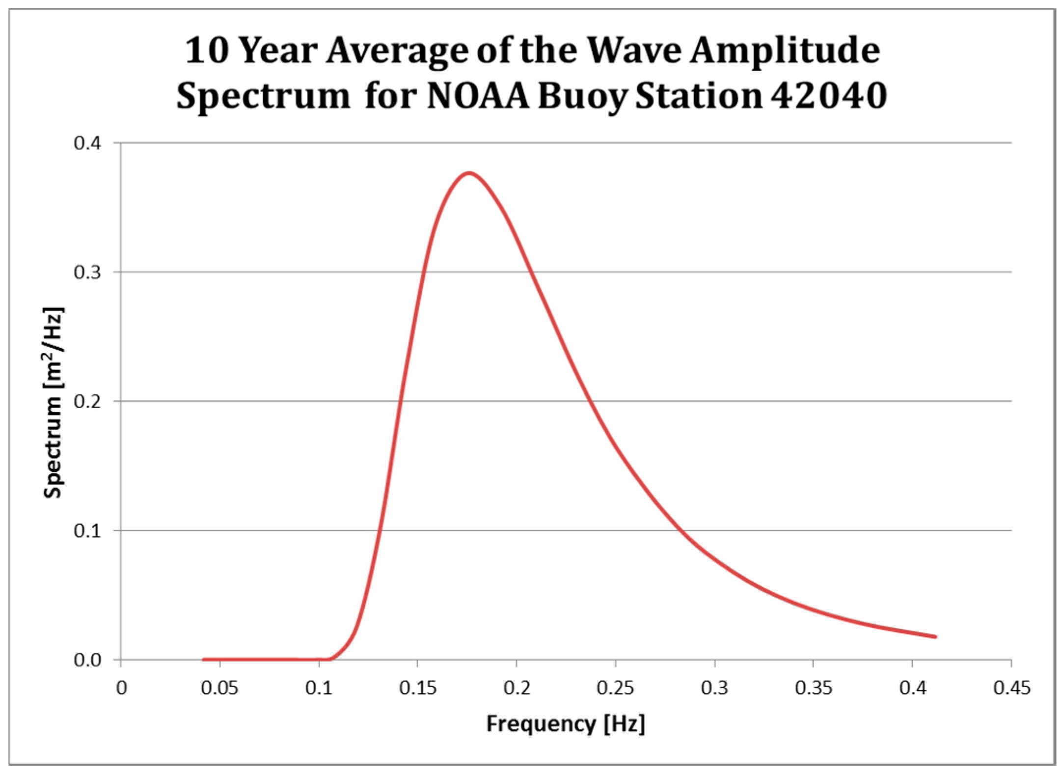
4. Calculated Results for a Localized Geographic Location

The method presented in this study was then used to estimate the available wave energy for the location of the NOAA National Data Buoy Center’s Station 42040 (LLNR 293)—Luke Offshore Test Platform, which is located about 64 nautical miles south of Dauphin Island, Alabama at 29°12’45”N, 88°12’27”W [24]. Once the data was analyzed following the steps described in Section 3, it was found that the 10-year (2003–2012) means for the significant wave height and peak wave period were Hs = 1.1 m and Tp = 5.7 s, respectively. A wave energy spectrum was then formulated based on these values (using Equation (9)), which will be used to assess that area for use with wave energy conversion technology.
In order to validate the wave energy predictions obtained from the presented approach, the calculated results were compared with the data from the NOAA National Data Buoy Center’s Station 42040—Luke Offshore Test Platform. The data is archived and disseminated by the National Data Buoy Center [27].
Based on the data, the monthly variation in the year 2012 for the available wave power (Equations (27) and (28)) is plotted in Figure 3 and compared with the monthly available wave power predictions derived from the 10-year average formulated using the approach presented in Section 3 and plotted in Figure 4. From that figure, it can be seen that both the annual mean power and the monthly power variation are in reasonably good agreement. Such agreement can also be seen in Table 1, which gives the % error of the predicted available wave power with respect to the actual wave power in 2012. From the comparison, it can be concluded that the wave energy estimates derived using the presented method are reliable, and the accuracy of the approach presented in this study is therefore validated. Table 1 also lists the results given by the EPRI method and demonstrates that the method employed by this study increases the accuracy of the EPRI method by an average factor of 1.1%.

5. Conclusions

A methodology, which was developed by EPRI based on a modified gamma spectrum, is presented and revised in this study and employed for analyzing the potential for wave energy conversion in a desired geographic area. This methodology allows WEC developers to easily and effectively predict the potential wave power available to their devices and, therefore, facilitate the prediction of power output performance (in a given year, season, month, etc.) in a specific location. The essential part of this methodology is the calibration of the spectral width parameter n and the spectral peakedness parameter γ. Compared to the original EPRI methodology, the revised method can yield results with a higher accuracy of 1.1% by using Hunt’s method to find the wavelength L. The presented methodology was then applied for the Luke Offshore Test Platform. The case study results showed that this method can deliver robust results in representing the wave climate in a given region where the WECs are deployed, and the estimates were close to the data disseminated by National Data Buoy Center.
It also needs to be mentioned that for a deployed WEC, there are two main factors that determine its power production, the wave source and the power takeoff (PTO) force/parameters [28,29]. Since the focus of this work is on the influence of wave climate resource on the output wave power, the PTO force/parameters are not included in the present model, which is a deficiency of this work and needs to be addressed in the future. In next phase, we will adopt the method developed by Salter [30] into the current model to also reflect the effects of power takeoff and torque limits on the wave power production. The enhanced methodology can be used to map and assess the ocean wave energy resource at any given geographical location in United States with higher accuracy and reliability.

Author Contributions

Jeremiah Pastorconducted this research as part of his Master thesis under the guidance of Yucheng Liu.

Conflicts of Interest

The authors declare no conflict of interest.

Appendix A

NCEP file structure for WaveWatch III Hindcast Data [19].
Figure A1. NCEP file structure for WaveWatch III Hindcast Data.
Sustainability 08 01321 g005

References

  1. Pastor, J.; Liu, Y.-C. Power absorption modeling and optimization of a point absorbing wave energy converter using numerical method. J. Energy Resour. Technol. 2014, 136, 021207. [Google Scholar] [CrossRef]
  2. Pastor, J.; Liu, Y.-C. Frequency and time domain modeling and power output for a heaving point absorber wave energy converter. Int. J. Energy Environ. Eng. 2014, 5, 1–13. [Google Scholar] [CrossRef]
  3. Water Power Technologies Office. Available online: http://www1.eere.energy.gov/water/hydrokinetic/default.aspx (accessed on 1 November 2016).
  4. Smith, G.; Taylor, J. Preliminary Wave Energy Device Performance Protocol. Available online: http://www.waveandtidalknowledgenetwork.com/ItemDetails.aspx?id=401 (accessed on 1 November 2016).
  5. Smith, G.H.; Venugopal, V.; Fasham, J. Wave spectral bandwidth as a measure of available wave power. In Proceedings of the 25th International Conference on Offshore Mechanics and Arctic Engineering, Hamburg, Germany, 1–9 June 2006.
  6. Fusco, F.; Nolan, G.; Ringwood, J.V. Variability reduction through optimal combination of wind/wave resources—An Irish case study. Energy 2010, 35, 314–325. [Google Scholar] [CrossRef]
  7. Folley, M.; Whittaker, T.J.T. Analysis of the nearshore wave energy resource. Renew. Energy 2009, 34, 1709–1715. [Google Scholar] [CrossRef]
  8. Carballo, R.; Iglesias, G. A methodology to determine the power performance of wave energy converters at a particular coastal location. Energy Convers. Manag. 2012, 61, 8–18. [Google Scholar] [CrossRef]
  9. Duclos, G.; Babarit, A.; Clement, A.H. Optimizing of power take off of a wave energy converter with regard to the wave climate. ASME J. Offshore Mech. Arct. Eng. 2006, 128, 56–64. [Google Scholar] [CrossRef]
  10. Sarmento, A.J.N.A.; Pontes, M.T.; Melo, A.B. The influence of the wave climate on the design annual production of electricity by OWC wave power plants. AASME J. Offshore Mech. Arct. Eng. 2003, 125, 139–144. [Google Scholar] [CrossRef]
  11. Electric Power Research Institute. Mapping and Assessment of the United States Ocean Wave Energy Resource; EPRI Technical Report 1024637; Electric Power Research Institute: Palo Alto, CA, USA, 2011. [Google Scholar]
  12. Bretschneider, C.L. Wave Variability and Wave Spectra for Wind Generated Gravity Waves; Technical Memo No. 118; Beach Erosion Board, US Army Corps of Engineering: Washington, DC, USA, 1959. [Google Scholar]
  13. Pierson, W.J.; Moskowitz, L. Proposed spectral form for fully developed wind seas based on the similarity theory of S.A. Kitaigorodskii. J. Geophys. Res. 1964, 69, 5181–5190. [Google Scholar] [CrossRef]
  14. Hasselmann, K.; Barnett, T.P.; Bouws, E.; Carlson, H.; Cartwright, D.E.; Enke, K.; Ewing, J.A.; Gienapp, H.; Hasselmann, D.E.; Kruseman, P.; et al. Measurements of Wind-Wave Growth and Swell Decay during the Joint North Sea Wave Project (JONSWAP); Deutches Hydrographisches Institut: Hamburg, Germany, 1973. [Google Scholar]
  15. Ochi, M.K.; Hubble, E.N. Six-parameter wave spectra. In Proceedings of the 15th Coastal Engineering Conference, Honolulu, HI, USA, 1–17 July 1976; pp. 301–328.
  16. Boukhanovsky, A.V.; Soares, C.G. Modelling of multipeaked directional wave spectra. Appl. Ocean Res. 2009, 31, 132–141. [Google Scholar] [CrossRef]
  17. Liu, Y.-C.; Cavalier, G.; Pastor, J.; Viera, R.J.; Guillory, C.; Judice, K.; Guiberteau, K.L.; Kozman, T.A. Design and construction of a wave generation system to model ocean conditions in the Gulf of Mexico. Int. J. Energy Technol. 2012, 4, 1–7. [Google Scholar]
  18. Guiberteau, K.L.; Liu, Y.-C.; Lee, J.; Kozman, T.A. Investigation of developing wave energy technology in the Gulf of Mexico. Distrib. Gener. Altern. Energy J. 2012, 27, 36–52. [Google Scholar] [CrossRef]
  19. MMAB Operational Wave Models. Available online: http://polar.ncep.noaa.gov/waves/#ww3products (accessed on 1 November 2016).
  20. Wavewatch III® Model. Available online: http://polar.ncep.noaa.gov/waves/wavewatch/wavewatch.shtml (accessed on 1 November 2016).
  21. Hsu, S.A.; Meindl, E.A.; Gilhousen, D.B. Determining the power-law wind-profile exponent under near-neutral stability conditions at sea. J. Appl. Meteorol. 1994, 33, 757–765. [Google Scholar] [CrossRef]
  22. ABP Marine Environmental Research. Atlas of UK Marine Renewable Energy Resources; Report R1106, Prepared for the UK Department of Trade and Industry; ABP Marine Environmental Research: Southampton, UK, 2004. [Google Scholar]
  23. Hagerman, G. Southern New England wave energy resource potential. In Proceedings of the Building Energy 2001, Boston, MA, USA, 23 March 2001.
  24. US Army Corps of Engineering. Direct Methods for Calculating Wavelength; Coastal Engineering Technical Note, CETN-1-17; US Army Corps of Engineering: Washington, DC, USA, 1985. [Google Scholar]
  25. Chen, H.-S.; Thompson, E.F. Interactive and Pade’s Solutions for the Water-Wave Dispersion Relation; Miscellaneous Paper CERC-85-4; US Army Engineer Waterways Experiment Station: Vicksburg, MI, USA, 1985. [Google Scholar]
  26. National Data Buoy Center, National Oceanic and Atmospheric Administration. Available online: http://www.ndbc.noaa.gov/station_page.php?station=42040 (accessed on 18 November 2013).
  27. Fenton, J.D.; McKee, W.D. On calculating the lengths of water waves. Coast. Eng. 1990, 14, 499–513. [Google Scholar] [CrossRef]
  28. Korde, U.A. A power take-off mechanism for maximizing the performance of an oscillating water column wave energy device. Appl. Ocean Res. 1991, 13, 75–81. [Google Scholar] [CrossRef]
  29. Wang, L.; Engstrom, J.; Leijon, M.; Isberg, J. Coordinated control of wave energy converters subject to motion constraints. Energies 2016, 9, 475. [Google Scholar] [CrossRef]
  30. Salter, S.H. Power conversion systems for ducks. In Proceedings of the International Conference on Future Energy Concepts, London, UK, 30 January–1 February 1979; pp. 100–108.
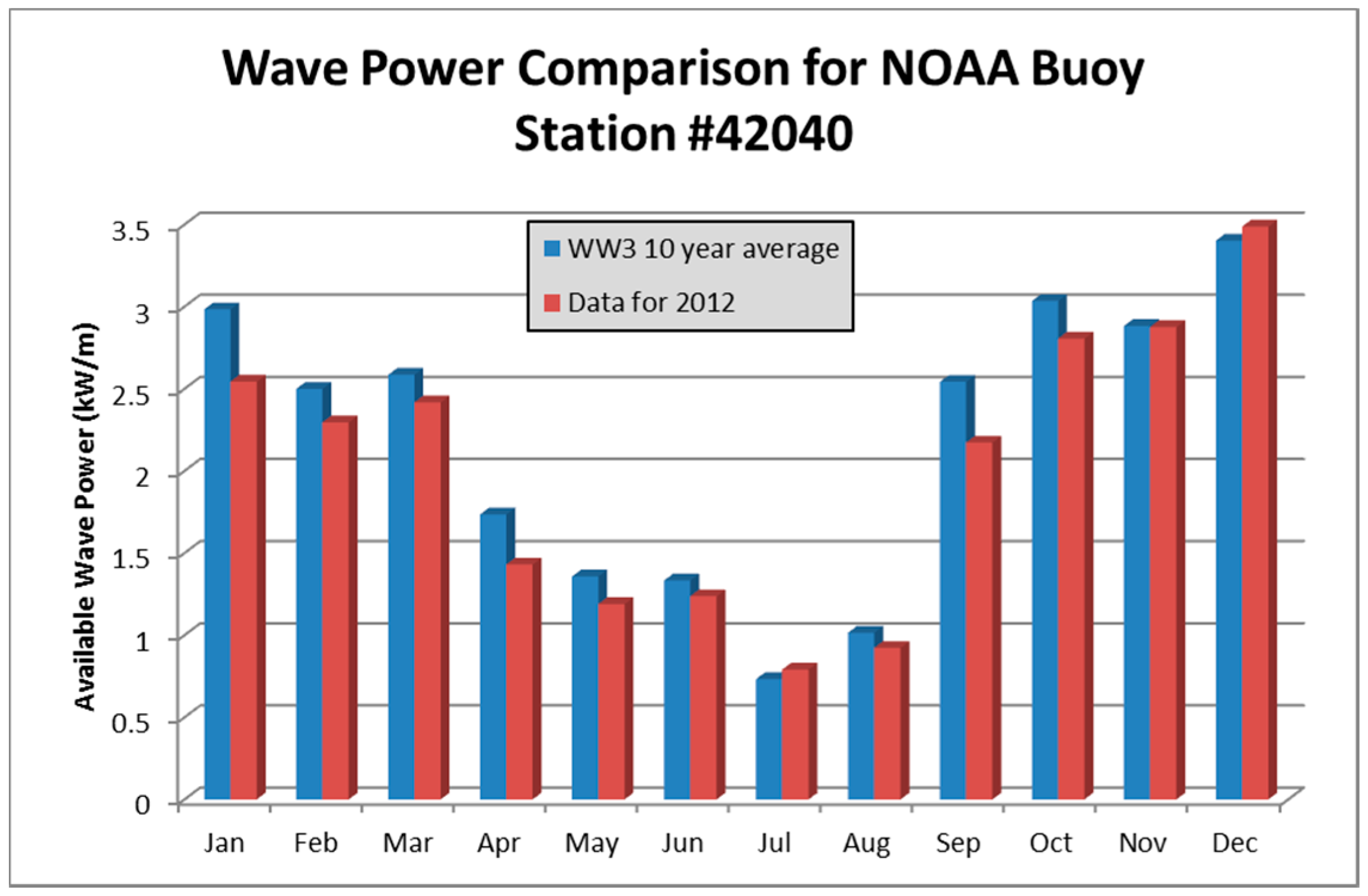
Figure 1. A flowchart of finding the wave power density and annual wave energy flux.
Sustainability 08 01321 g001
Figure 2. Process for calibrating theoretical spectra reconstructed from sea state parameters.
Sustainability 08 01321 g002
Figure 3. Monthly variation in wave power for NOAA buoy station #42040.
Sustainability 08 01321 g003
Figure 4. Ten-year means of the wave energy for National Oceanic and Atmospheric Administration’s (NOAA’s) buoy station #42040 with wave height (Hs) = 1.1 m and peak wave period (Tp) = 5.7 s.
Sustainability 08 01321 g004
Table 1. Error percentage of the predicted available wave power density with respect to the actual available wave power density in 2012.
MonthPredicted Power (kW/m)NOAA Data [24] (kW/m)ErrorEPRI Data [11] (kW/m)Error
January2983.572543.2114.8%2523.1615.4%
February2499.122295.208.2%2291.248.3%
March2585.302416.696.5%2412.196.7%
April1735.201429.9917.6%1395.9919.5%
May1357.281189.0412.4%1119.2417.5%
June1333.041237.117.2%1231.697.6%
July733.10791.117.3%799.128.3%
August1014.97922.539.1%909.5410.4%
September2542.292172.3714.6%2121.4516.6%
October3034.142805.237.5%2794.997.9%
November2882.432875.590.2%2865.410.6%
December3401.583487.742.5%3499.522.8%
Average2175.172013.829.0%1996.9610.1%

