
Examining Determinants of CO2 Emissions in 73 Cities in China


Abstract
:1. Introduction
2. Estimating CO2 Emissions of 73 Cities from 2002 to 2012 and Their Relations with GDP Per Capita
2.1. Estimating CO2 Emissions
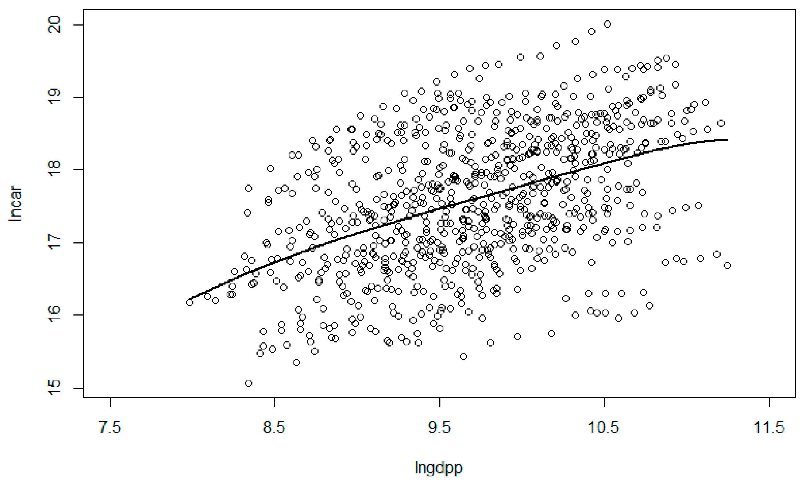
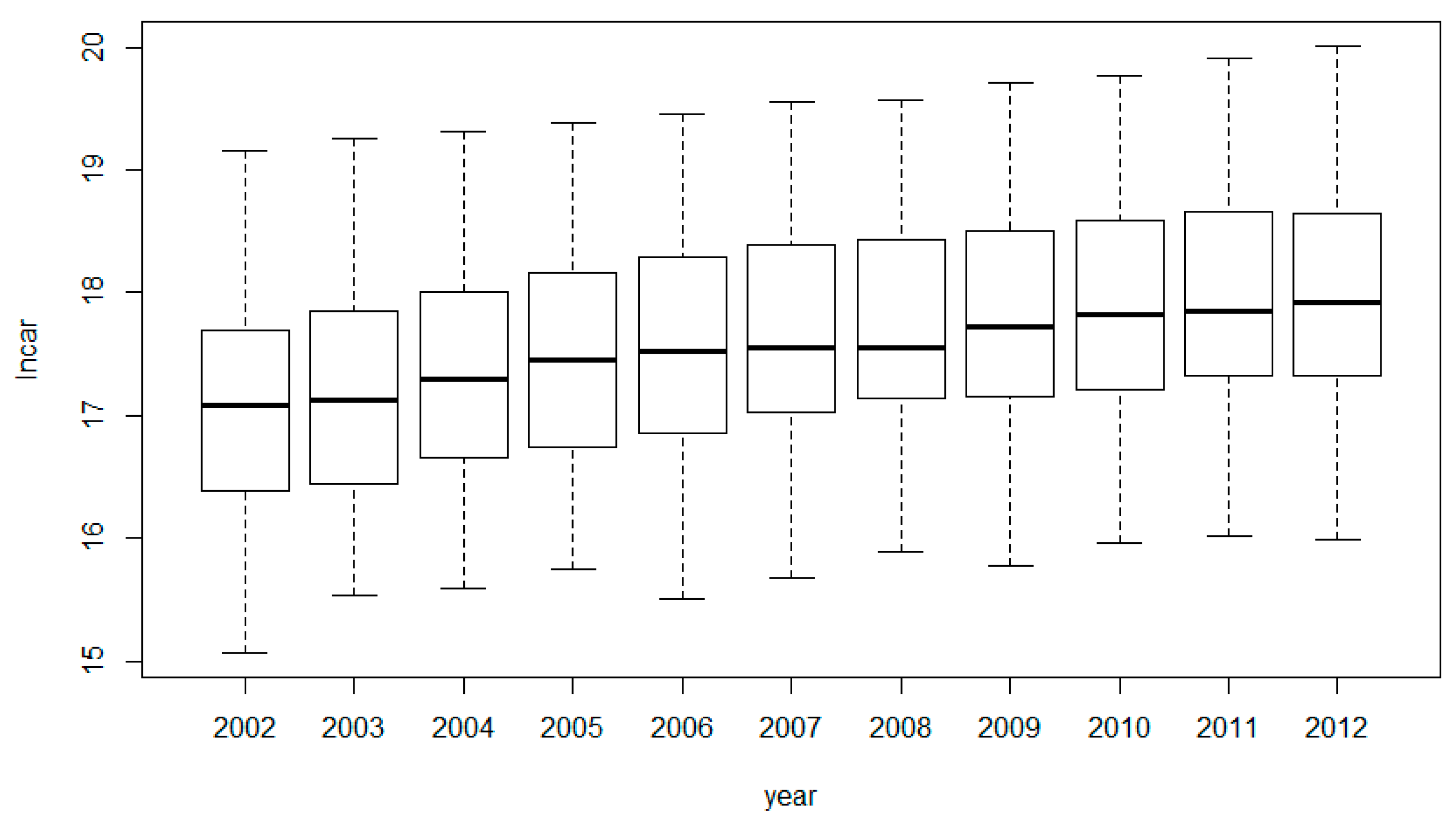
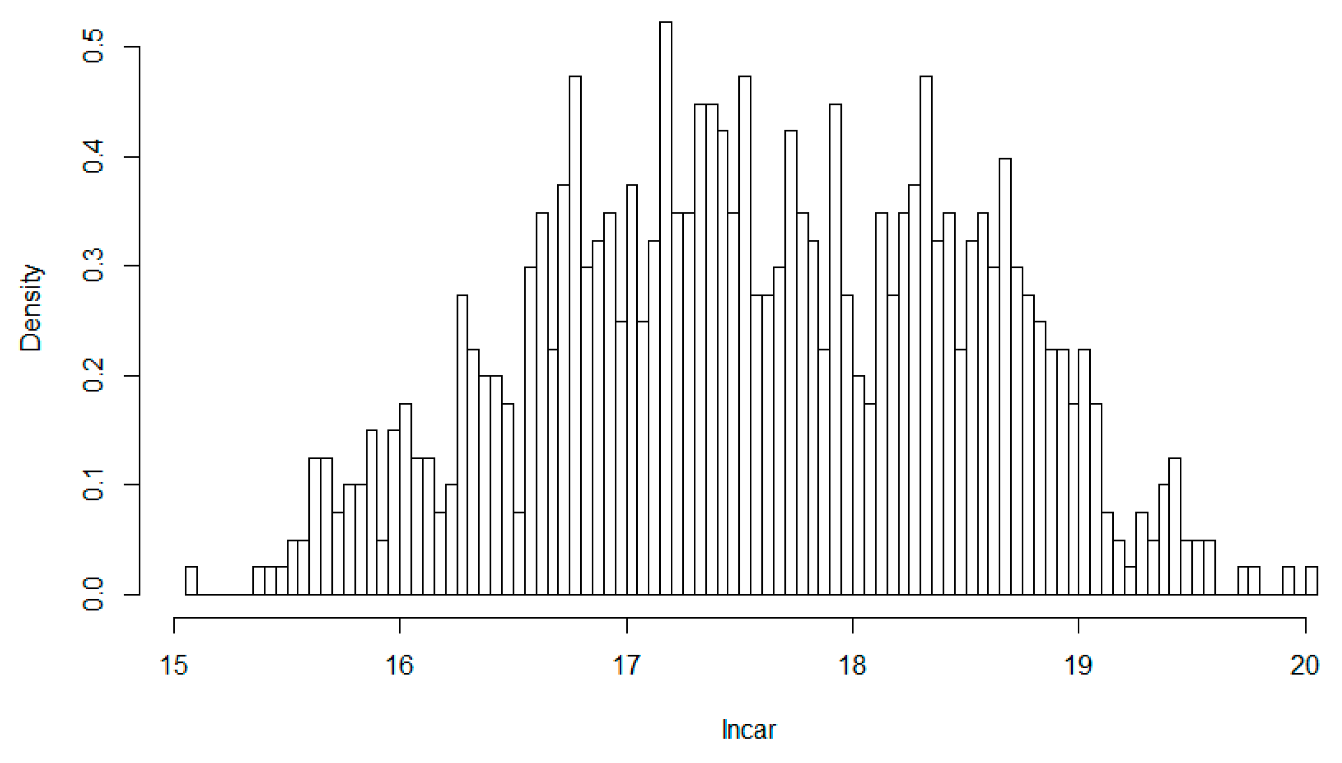
2.2. Descriptive Analysis
3. Models
3.1. STIRPAT Model and its Extended Model
3.2. Linear Mixed Effect Model
4. Data
5. Empirical Results
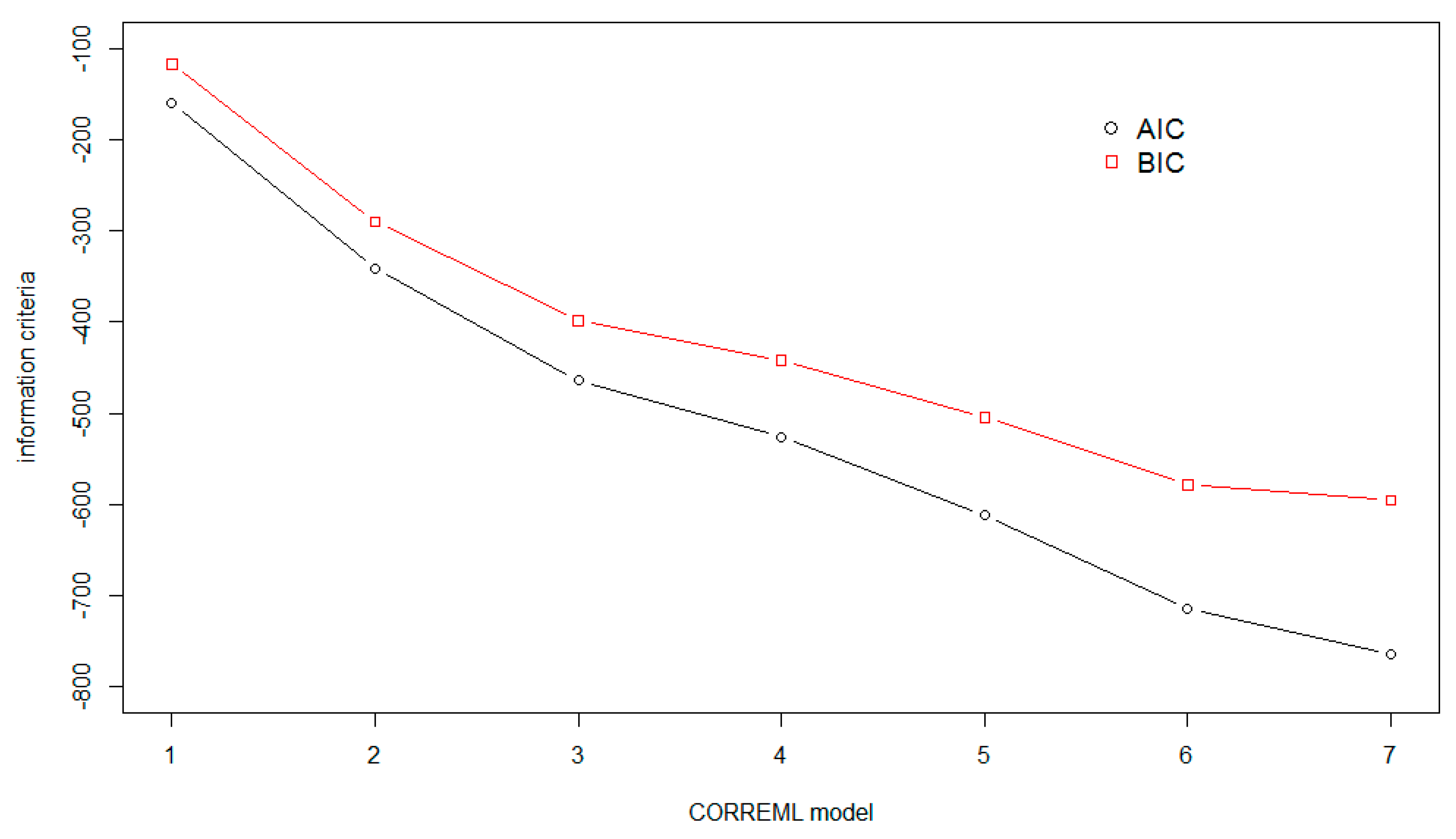
5.1. Model Selection
5.2. Empirical Results
6. Conclusions
Acknowledgments
Author Contributions
Conflicts of Interest
References
- Carlsson, F.; Lundström, S. The Effects of Economic and Political Freedom on CO2 Emissions; Economic Studies, Department of Economics, School of Economics and Commercial Law, Göteborg University: Gothenburg, Sweden, 2003; p. 79. [Google Scholar]
- Quadrelli, R.; Peterson, S. The energy–climate challenge: Recent trends in CO2 emissions from fuel combustion. Energy Policy 2007, 35, 5938–5952. [Google Scholar] [CrossRef]
- Shi, A. The impact of population pressure on global carbon dioxide emissions, 1975–1996: Evidence from pooled cross-country data. Ecol. Econ. 2003, 44, 29–42. [Google Scholar] [CrossRef]
- Fan, Y.; Liu, L.-C.; Wu, G.; Wei, Y.-M. Analyzing impact factors of CO2 emissions using the stirpat model. Environ. Impact Assess. Rev. 2006, 26, 377–395. [Google Scholar] [CrossRef]
- Liao, H.; Cao, H.-S. How does carbon dioxide emission change with the economic development? Statistical experiences from 132 countries. Glob. Environ. Chang. 2013, 23, 1073–1082. [Google Scholar] [CrossRef]
- Poumanyvong, P.; Kaneko, S. Does urbanization lead to less energy use and lower CO2 emissions? A cross-country analysis. Ecol. Econ. 2010, 70, 434–444. [Google Scholar] [CrossRef]
- Lin, S.; Zhao, D.; Marinova, D. Analysis of the environmental impact of China based on stirpat model. Environ. Impact Assess. Rev. 2009, 29, 341–347. [Google Scholar] [CrossRef]
- Zhu, Q.; Peng, X.; Lu, Z.; Yu, J. Analysis model and empirical study of impacts from population and consumption on carbon emissions. China Popul. Resour. Environ. 2010, 20, 98–102. [Google Scholar]
- Li, H.; Mu, H.; Zhang, M.; Gui, S. Analysis of regional difference on impact factors of China’s energy–related CO2 emissions. Energy 2012, 39, 319–326. [Google Scholar] [CrossRef]
- Song, X.; Zhang, Y.; Wang, Y.; Feng, Y. Analysis of impacts of demographic factors on carbon emissions based on the ipat model. Res. Environ. Sci. 2012, 5, 109–115. [Google Scholar]
- Li, H.; Mu, H.; Zhang, M.; Li, N. Analysis on influence factors of China’s CO2 emissions based on path–stirpat model. Energy Policy 2011, 39, 6906–6911. [Google Scholar] [CrossRef]
- Zhu, Q.; Peng, X. The impacts of population change on carbon emissions in China during 1978–2008. Environ. Impact Assess. Rev. 2012, 36, 1–8. [Google Scholar] [CrossRef]
- Wei, T. What stirpat tells about effects of population and affluence on the environment? Ecol. Econ. 2011, 72, 70–74. [Google Scholar] [CrossRef]
- Wang, M.; Che, Y.; Yang, K.; Wang, M.; Xiong, L.; Huang, Y. A local-scale low-carbon plan based on the stirpat model and the scenario method: The case of minhang district, shanghai, china. Energy Policy 2011, 39, 6981–6990. [Google Scholar] [CrossRef]
- Shao, S.; Yang, L.-L.; Cao, J.-H. Study on influencing factors of CO2 emissions from industrial energy consumption: An empirical analysis based on stirpat model and industrial sectors’ dynamic panel data in Shanghai. J. Financ. Econ. 2010, 11, 16–27. [Google Scholar]
- Wang, Z.; Yin, F.; Zhang, Y.; Zhang, X. An empirical research on the influencing factors of regional CO2 emissions: Evidence from Beijing city, China. Appl. Energy 2012, 100, 277–284. [Google Scholar] [CrossRef]
- Wang, P.; Wu, W.; Zhu, B.; Wei, Y. Examining the impact factors of energy-related CO2 emissions using the stirpat model in Guangdong province, China. Appl. Energy 2013, 106, 65–71. [Google Scholar] [CrossRef]
- Liang, J.; Zheng, W.; Cai, J. The decomposition of energy consumption growth in China: Based on input–output model. J. Natl. Resour. 2007, 22, 853–864. [Google Scholar]
- Ehrlich, P.; Holdren, J. The people problem. Saturday Rev. 1970, 4, 42–43. [Google Scholar]
- Ehrlich, P.; Holdren, J. A bulletin dialogue on the ‘closing circle’. Critique: One dimensional ecology. Bull. At. Sci. 1972, 28, 16–27. [Google Scholar]
- Dietz, T.; Rosa, E.A. Rethinking the environmental impacts of population, affluence and technology. Hum. Ecol. Rev. 1994, 1, 277–300. [Google Scholar]
- York, R.; Rosa, E.A.; Dietz, T. Stirpat, ipat and impact: Analytic tools for unpacking the driving forces of environmental impacts. Ecol. Econ. 2003, 46, 351–365. [Google Scholar] [CrossRef]
- Zhang, Z. Why did the energy intensity fall in China’s industrial sector in the 1990s? The relative importance of structural change and intensity change. Energy Econ. 2003, 25, 625–638. [Google Scholar] [CrossRef]
- Ang, B.W. The lmdi approach to decomposition analysis: A practical guide. Energy Policy 2005, 33, 867–871. [Google Scholar] [CrossRef]
- Wang, C.; Chen, J.; Zou, J. Decomposition of energy-related CO2 emission in China: 1957–2000. Energy 2005, 30, 73–83. [Google Scholar] [CrossRef]
- Tan, Z.; Li, L.; Wang, J.; Wang, J. Examining the driving forces for improving China’s CO2 emission intensity using the decomposing method. Appl. Energy 2011, 88, 4496–4504. [Google Scholar] [CrossRef]
- Liu, X.Q.; Ong, H.L. The application of the divisia index to the decomposition of changes in industrial energy consumption. Energy J. 1992, 13, 161–178. [Google Scholar] [CrossRef]
- Ang, B.W.; Liu, F.L.; Chung, H.S. A generalized fisher index approach to energy decomposition analysis. Energy Econ. 2004, 26, 757–763. [Google Scholar] [CrossRef]
- Kaya, Y. Impact of Carbon Dioxide Emission Control on GNP Growth: Interpretation of Proposed Scenarios; IPCC Energy and Industry Subgroup, Response Strategies Working Group: Paris, France, 1990; Volume 76. [Google Scholar]
- Yang, S. Primary study on effect of C-O balance of afforestatal trees in cities. Urban Environ. Urban Ecol. 1996, 1, 37–39. [Google Scholar]
- Rosa, E.A.; Dietz, T. Climate change and society speculation, construction and scientific investigation. Int. Sociol. 1998, 13, 421–455. [Google Scholar] [CrossRef]
- Eisenhart, C. The assumptions underlying the analysis of variance. Biometrics 1947, 3, 1–21. [Google Scholar] [CrossRef] [PubMed]
- Laird, N.M.; Ware, J.H. Random-effects models for longitudinal data. Biometrics 1982, 963–974. [Google Scholar] [CrossRef]
- West, B.T.; Welch, K.B.; Galecki, A.T. Linear Mixed Models: A Practical Guide Using Statistical Software; CRC Press: Boca Raton, FL, USA, 2014. [Google Scholar]
- Huang, J. Regional Price Difference and Calculation of the Regional Economic Disparity; Jinan University: Guangzhou, China, 2010. [Google Scholar]
- Hsiao, C.; Sun, B.-H. To pool or not to pool panel data. In Panel Data Econometrics: Future Directions; Springer: Berlin/Heidelberg, Germany, 2000. [Google Scholar]
- Gurka, M.J. Selecting the best linear mixed model under reml. Am. Stat. 2006, 60, 19–26. [Google Scholar] [CrossRef]
- Steele, R. Model selection for multilevel models. In The Sage Handbook of Multilevel Modeling; Scott, M.A., Simonoff, J.S., Marx, B.D., Eds.; SAGE Publications Ltd.: London, UK, 2013. [Google Scholar]
- Akaike, H. Information theory and an extension of the maximum likelihood principle. Int. Symp. Inform. Theory 1973, 1, 610–624. [Google Scholar]
- Schwarz, G. Estimating the dimension of a model. Ann. Stat. 1978, 6, 15–18. [Google Scholar] [CrossRef]
- Harville, D.A. Bayesian inference for variance components using only error contrasts. Biometrika 1974, 61, 383–385. [Google Scholar] [CrossRef]
- Martinez-Zarzoso, I.; Maruotti, A. The environmental kuznets curve: Functional form, time-varying heterogeneity and outliers in a panel setting. Environmetrics 2013, 24, 461–475. [Google Scholar] [CrossRef]


| Independent Variables | Definition | Unit of Measurement | Data Source |
|---|---|---|---|
| Population (apop) | Average annual resident population | Ten thousand people | China Statistical Yearbook for Regional Economy, The Fifth National Census of Population, The Sixth National Census of Population |
| Urbanization (urb) | Percent of the urban population in resident population | — | China Statistical Yearbook for Regional Economy |
| Share of industry in GDP (ind) | Share of valued added in secondary industry | — | China Statistical Yearbook for Regional Economy |
| Energy consumption structure (enc) | Share of coal consumption in energy consumption | — | City’s Statistical Yearbook |
| Real GDP per capita (gdpp) | Gross domestic product divided by population | Yuan per capita (2002 Beijing price) | City’s Statistical Yearbook, China Statistical Yearbook for Regional Economy |
| Year | Statistics | car | apop | urb | ind | enc | gdpp |
|---|---|---|---|---|---|---|---|
| 2002 | Mean | 35,098,993 | 572.60 | 0.41 | 0.47 | 0.50 | 10,421 |
| (Std.Dev.) | (34,354,369) | (391.53) | (0.22) | (0.08) | (0.20) | (6319) | |
| 2003 | Mean | 40,565,026 | 578.72 | 0.43 | 0.47 | 0.50 | 11,724 |
| (Std.Dev.) | (39,703,731) | (395.19) | (0.22) | (0.08) | (0.20) | (6962) | |
| 2004 | Mean | 47,663,501 | 583.06 | 0.44 | 0.51 | 0.52 | 13,369 |
| (Std.Dev.) | (45,437,913) | (398.11) | (0.22) | (0.09) | (0.20) | (7901) | |
| 2005 | Mean | 54,375,314 | 587.67 | 0.45 | 0.50 | 0.56 | 15,152 |
| (Std.Dev.) | (51,516,301) | (402.15) | (0.22) | (0.10) | (0.21) | (8877) | |
| 2006 | Mean | 60,997,341 | 593.36 | 0.47 | 0.52 | 0.56 | 17,168 |
| (Std.Dev.) | (57,050,867) | (407.86) | (0.21) | (0.11) | (0.21) | (9995) | |
| 2007 | Mean | 67,172,395 | 601.25 | 0.46 | 0.52 | 0.56 | 19,500 |
| (Std.Dev.) | (61,980,922) | (416.31) | (0.22) | (0.09) | (0.21) | (11,133) | |
| 2008 | Mean | 68,399,980 | 609.54 | 0.47 | 0.53 | 0.55 | 21,623 |
| (Std.Dev.) | (62,469,073) | (425.90) | (0.22) | (0.10) | (0.21) | (11,995) | |
| 2009 | Mean | 7,341,6321 | 617.89 | 0.49 | 0.51 | 0.55 | 23,867 |
| (Std.Dev.) | (66,664,326) | (436.35) | (0.23) | (0.10) | (0.22) | (12,718) | |
| 2010 | Mean | 80,330,273 | 628.58 | 0.50 | 0.52 | 0.56 | 26,561 |
| (Std.Dev.) | (73,077,369) | (451.03) | (0.23) | (0.10) | (0.24) | (13,564) | |
| 2011 | Mean | 86,270,459 | 642.13 | 0.50 | 0.52 | 0.56 | 29,061 |
| (Std.Dev.) | (79,446,312) | (461.69) | (0.22) | (0.10) | (0.24) | (14,649) | |
| 2012 | Mean | 87,470,249 | 651.90 | 0.51 | 0.51 | 0.55 | 31,727 |
| (Std.Dev.) | (81,821,182) | (467.18) | (0.23) | (0.10) | (0.25) | (15,970) |
| Model | Variable(s) Contained in Random Effect Design Matrix |
|---|---|
| CORREML1 | Intercept |
| CORREML2 | Intercept + lnapop |
| CORREML3 | Intercept + lnapop + lnurb |
| CORREML4 | Intercept + lnapop + lnurb + lnind |
| CORREML5 | Intercept + lnapop + lnurb + lnind + lnenc |
| CORREML6 | Intercept + lnapop + lnurb + lnind + lnenc + lngdpp |
| CORREML7 | Intercept + lnapop + lnurb + lnind + lnenc + lngdpp + (lngdpp)2 |
| Variable | Intercept | lnapop | lnurb | lnind | lnenc | lngdpp | (lngdpp)2 |
|---|---|---|---|---|---|---|---|
| Coefficient | −9.893 ** | 0.585 *** | 0.041 | 0.567 *** | 0.204 *** | 4.359 *** | −0.190 *** |
| Goodness of fit | R2 = 0.995 | Adjusted R2 = 0.995 | |||||
| Variable | Intercept | lnapop | lnurb | lnind | lnenc | lngdpp | (lngdpp)2 |
|---|---|---|---|---|---|---|---|
| Intercept | 25.959 | ||||||
| lnapop | –0.154 | 0.580 | |||||
| lnurb | 0.135 | 0.407 | 0.161 | ||||
| lnind | –0.197 | –0.075 | 0.661 | 0.585 | |||
| lnenc | 0.704 | –0.070 | 0.068 | –0.230 | 0.331 | ||
| lngdpp | –0.996 | 0.078 | –0.190 | 0.177 | –0.686 | 5.399 | |
| (lngdpp)2 | 0.996 | –0.120 | 0.212 | –0.139 | 0.668 | –0.998 | 0.283 |
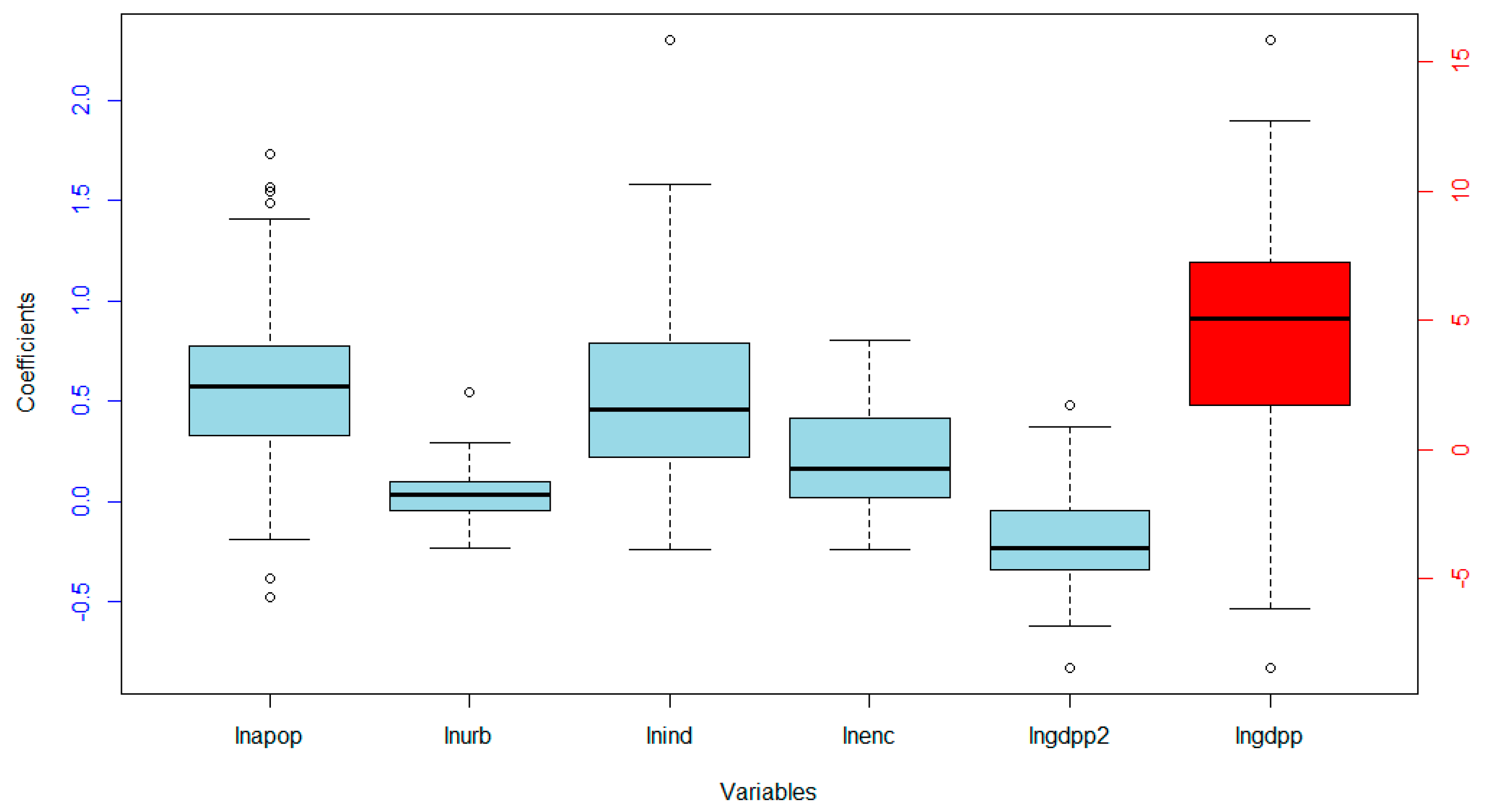
| Statistics | lnapop | lnurb | lnind | lnenc | lngdpp | (lngdpp)2 |
|---|---|---|---|---|---|---|
| Lower whisker | –0.189 | –0.234 | –0.240 | –0.236 | –6.164 | –0.619 |
| 25% percentile | 0.331 | –0.043 | 0.218 | 0.019 | 1.714 | –0.339 |
| Median | 0.575 | 0.033 | 0.460 | 0.163 | 5.079 | –0.230 |
| Mean | 0.585 | 0.041 | 0.567 | 0.204 | 4.359 | –0.190 |
| Standard deviation | 0.447 | 0.129 | 0.488 | 0.259 | 4.717 | 0.248 |
| 75% percentile | 0.778 | 0.099 | 0.793 | 0.412 | 7.228 | –0.049 |
| Upper whisker | 1.408 | 0.294 | 1.581 | 0.804 | 12.720 | 0.370 |
| Item | Group I | Group II | Group III | |
|---|---|---|---|---|
| Mean values in year 2012 | apop | 518.73 | 671.78 | 701.72 |
| urb | 0.4724 | 0.4974 | 0.6122 | |
| ind | 0.5180 | 0.5352 | 0.4984 | |
| enc | 0.6859 | 0.5128 | 0.5077 | |
| gdpp | 29,713.06 | 30,504.74 | 41,497.09 | |
| carbon per capita | 9.94 | 14.75 | 12.83 | |
| Estimated GDP per capita at emission peak | 2786.16 | 49,405.26 | 527,326.40 | |
© 2016 by the authors; licensee MDPI, Basel, Switzerland. This article is an open access article distributed under the terms and conditions of the Creative Commons Attribution (CC-BY) license (http://creativecommons.org/licenses/by/4.0/).
Share and Cite
Zheng, H.; Hu, J.; Guan, R.; Wang, S. Examining Determinants of CO2 Emissions in 73 Cities in China. Sustainability 2016, 8, 1296. https://doi.org/10.3390/su8121296
Zheng H, Hu J, Guan R, Wang S. Examining Determinants of CO2 Emissions in 73 Cities in China. Sustainability. 2016; 8(12):1296. https://doi.org/10.3390/su8121296
Chicago/Turabian StyleZheng, Haitao, Jie Hu, Rong Guan, and Shanshan Wang. 2016. "Examining Determinants of CO2 Emissions in 73 Cities in China" Sustainability 8, no. 12: 1296. https://doi.org/10.3390/su8121296