Computational Fluid Dynamic Modelling of Thermal Periodic Stabilized Regime in Passive Buildings

Abstract

The periodic stabilized regime is the condition where the temperature of each point of a certain environment varies following a periodic law. This phenomenon occurs in many practical applications, such as passive or ancient buildings not equipped with Heating, Ventilating and Air Conditioning HVAC systems and located in latitudes where the temperature greatly varies with Earth’s daily cycles. Despite that, the study of transient phenomena is often simplified, i.e., considering negligible the thermal response of the indoor microclimate. An exact solution to enclosures whose microclimate is free to evolve under a periodic stabilized regime does not exist nowadays, also from an analytical point of view. The aim of this study is to parametrically analyze the thermal variations inside a room when a transient periodic temperature is applied on one side. The phenomenon has been numerically studied through Computational Fluid Dynamics (CFD) and analytically validated using a function that reproduces the daily variation of the outdoor temperature. The results of this research would lay the groundwork to develop analytical correlations to solve and predict the thermal behavior of environments subject to a periodic stabilized regime.

1. Introduction

The indoor microclimate of buildings is greatly influenced by outdoor climate conditions and by the ability of the architectural envelope to dampen them. These physical phenomena involve different heat transfer processes (coupling convection/conduction) which can affect several aspects related to sustainable architecture and design of buildings and cities, such as the reduction of energy demand [1,2,3,4,5,6], the decrease of the environmental impact [7,8] and the analysis of the urban canyon effect [9,10]. Differentially heated enclosures have been widely studied in the past [11,12,13,14,15]. However, the complexity of the problem has led the researchers to apply several simplifications in the analysis of these phenomena, such as setting the outdoor conditions as steady or considering indoor microclimate as a controlled environment (where the interior conditions are set, and, if required, dynamically controlled by an HVAC system). Furthermore, the ISO 13786:2007(E) [16] supplies the procedure for the calculation of the dynamic thermal behavior of building components imposing the temperature on one side of the element as constant.

Time-periodic thermal conditions should be taken into account especially when the outdoor temperature greatly varies during the day [17,18,19,20,21]. One application is the so-called periodic stabilized regime, which is the condition where the average temperature varies with a periodic law in each point of a certain environment. This phenomenon finds practical applications in buildings not characterized by HVAC systems, as passive, ancient and/or historical buildings, where the temperature is free to evolve without thermal constraints.

The problem has been analytically studied taking into account the case of the semi-infinite solid [22,23,24]. An analytical solution for the transient temperature distribution in a semi-infinite solid is known only for three surface conditions: constant surface temperature, constant surface heat flux, and surface convection. To the best of our knowledge, there is not an exact analytical law to predict the indoor thermal behavior in enclosures where a varying temperature is applied at least on one external surface and the indoor temperature is free to evolve.

Time-periodic natural convection in 2D enclosures has been also numerically examined in the past literature [25,26,27,28,29,30,31,32]. However, these studies are more focused on the analysis of the fluid field inside the enclosure rather than supplying new analytical relations to solve the physical phenomenon of the periodic stabilized regime. This problem could be studied by coupling experimental measures and numerical simulations and comparing the results. Despite that, an experimental approach is not always applicable, for example when the case study is too complex to be experimentally duplicated or when no more existing buildings or sites are analyzed [33,34].

The aim of this study is to parametrically analyze the thermal variations inside a room when a transient periodic temperature is applied on one side. The results of this research would lay the groundwork to develop analytical correlations to solve and predict the thermal behavior of environments subject to time-dependent thermal forcing and where the indoor temperature is free to evolve, matching together all the approaches used up to now.

2. Materials and Methods

Nowadays, Computational Fluid Dynamic (CFD) is one of the main tools used in several studies to analyze heat transfer processes involving convection and conduction. However, these studies did not supply analytical correlations to predict the thermal behavior of enclosures where the temperature is free to evolve under a periodic stabilized regime. In this work, the indoor temperature trends inside the model of a simple room has been numerically investigated through CFD. Parametric analyses have been carried out by changing the thermo-physical and boundary conditions of the case study. Several sets of simulations have been, indeed, taken into account in order to understand what the thermal behavior of the indoor environment is when geometry and thermal inputs vary. Four sensitivity tests have been carried out changing one parameter at a time. All the case studies analyzed are summarized in

Table 1. Case studies summary.

Case Name	Sensitivity Test
Case 1	Material of the solid domain
Case 2	Thickness of the solid domain
Case 3	External sinusoidal temperature Tsin
Case 4	External fixed temperature Twall

.

In the first two cases (Case 1 and Case 2), the thermo-physical properties of the envelope have been varied, while in the last two cases (Case 3 and Case 4), different thermal inputs have been applied on the sidewalls of the model. The varying profile of the external daily temperature has been reproduced through a sinusoidal trend on the external surface of the enclosure.

2.1. Analytical Statement

In the study of heat transfer by conduction, the Fourier’s equation admits analytical solutions only for well-defined problems, usually characterized by simple geometries, simple boundary conditions, materials with uniform properties and independent temperature [22,23,24].

Many heat transfer problems are time-dependent. It is possible to analyze transient conduction phenomena referring to a semi-infinite solid that extends its dimensions to infinity with the exception of one of them.

A typical case of transient conduction is described by a body of a wide thickness delimited by a flat surface where a transient periodic temperature is imposed on. The other surfaces of the solid are at a distance large enough not to consider their influence. The temperature in all the points of the body varies with the same periodic law of the imposed temperature after a certain time. This condition is called periodic stabilized regime.

Suppose to analyze a semi-infinite wall, whose material is homogeneous and isotropic, delimited by a plan surface. The thermo-physical characteristics of the medium (c_p, λ, ρ) are independent from temperature and time. Imagine to impose on its surfaces a sinusoidal temperature in the normal x direction, which follows the analytical Equation (1):

$$T(x,\tau )=T_m+\mathrm{\Theta }\sin (\omega \tau )$$

(1)

After an initial transient period, the temperature reaches a periodic stabilized regime. Considering a time τ in the periodic stabilized regime, since the temperature does not depend on the spatial coordinates y and z, the solution to the Fourier’s equation is (2):

$$T(x,\tau )=T_m+\mathrm{\Theta }{e}^{-\beta x}\sin (\omega \tau -\beta x)$$

(2)

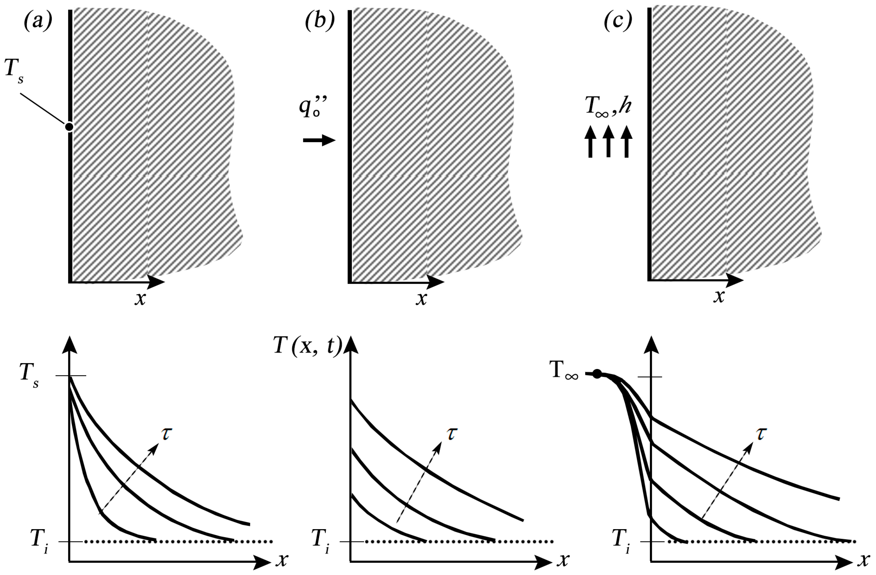
Transient conduction in a semi-infinite solid can be solved also in three different conditions on the surface [24]: a constant temperature T_s ≠ T_i (Figure 1a); a constant heat flux $q_0^{″}$ (Figure 1b); an exposure to a fluid whose temperature is T_∞ ≠ T_i and a convective coefficient h (Figure 1c).

These three cases can be solved respectively through the following equations [24]:

$$\frac{T(x,\tau )-T_s}{T_i-T_s}=erf\left(\frac{x}{2\sqrt{\alpha \tau }}\right)$$

(3)

$$T(x,\tau )-T_i=\frac{2q_0^{″}{(\alpha \tau /\pi )}^{1/2}}{\lambda }\exp \left(\frac{-x^2}{4\alpha \tau }\right)-\frac{q_0^{″}x}{\lambda }erfc\left(\frac{x}{2\sqrt{\alpha \tau }}\right)$$

(4)

$$\frac{T(x,\tau )-T_i}{T_{\infty }-T_i}=erfc\left(\frac{x}{2\sqrt{\alpha \tau }}\right)-\left[\exp \left(\frac{hx}{\lambda }+\frac{h^2\cdot \alpha \tau }{{\lambda }^2}\right)\right]\cdot \left[erfc\left(\frac{x}{2\sqrt{\alpha \tau }}+\frac{h\sqrt{\alpha \tau }}{\lambda }\right)\right]$$

(5)

The mathematical calculations to obtain the Equations (3)–(5) can be found in [22,23,24].

The thermo-physical characteristics of the solid body, such as the diffusivity, the phase lag and the thermal damping factor, are noticeable in all the equations. It means that the initial sinusoidal temperature is attenuated and delayed proportionally to the thickness and the physical and thermal properties of the wall.

To the best of our knowledge, an analytical solution to enclosures subject to a periodic stabilized regime does not exist nowadays.

2.2. Numerical Approach

The commercial software Ansys Fluent v. 14.5 [35] has been used for the transient simulations. The governing equations used for the gas phase are the unsteady form of the continuity, compressible Navier–Stokes, and energy equations for a perfect gas with the Sutherland model for the viscosity and temperature-dependent properties. The equations that govern the phenomenon (momentum (6), continuity (7) and energy conservation (8)) can be expressed as follows:

$${\overline{u}}_j\frac{\partial {\overline{u}}_i}{\partial x_j}=-\frac{1}{\rho }\frac{\partial \overline{p}}{\partial x_i}+\frac{\mu }{\rho }\frac{{\partial }^2{\overline{u}}_i}{\partial x_i\partial x_j}-\frac{\partial }{\partial x_j}\left({\overline{u}}_i^{\prime }{\overline{u}}_j^{\prime }\right)+g_i$$

(6)

$$\frac{\partial {\overline{u}}_i}{\partial x_i}=0$$

(7)

$${\overline{u}}_i\frac{\partial \overline{T}}{\partial x_i}+\frac{\partial }{\partial x_i}\left(k\frac{\partial \overline{T}}{\partial x_i}\right)=0$$

(8)

where i = 1, 2, 3 for the three-dimensional (3D) case and i = 1, 2 for the two-dimensional (2D) case. The Fourier law has been used for the analysis of the solid body.

Time-accurate solutions have been obtained using the implicit coupled scheme with second-order accuracy in time with the SIMPLE (Semi-Implicit Method for Pressure-Linked Equations) segregated scheme, used for the gas phase until convergence was achieved. For time-accurate solutions, the fluxes for all equations at the cell faces have been interpolated by using the second-order upwind scheme. Pressure equation and the Laplace equation for the conduction have been also computed by using second-order accuracy. The Boussinesq approach has been applied to the model and RNG k-ε turbulence model [36,37] has been chosen to study the fluid turbulence after the calculation of the dimensionless groups for the natural convection (Ra = 2.54 × 10¹⁰). Basing on convergence and computational stability criteria, the RNG k-ε model has been considered the most suitable for this case in terms of indoor flow field characterization [38]. The simulations have run with the unsteady regime with an initial time step size between 10⁻⁷ and 10⁻⁵ s and it has been increased at 20 s after the residuals have reached the stability. This time step has been obtained after several tests based on numerical stability and numerical residual convergence. Convergence criteria have been reached when all the residuals were below 10⁻⁶.

3. Validation Cases

Heat conduction problems are often solved through many assumptions and simplifications, such as the steady state condition. Despite that, several applications involve time-dependent variation of the temperature, especially when it changes in a periodic manner. As previously said, there is not an exact analytical law to predict the indoor thermal behavior in enclosures where the indoor temperature is free to evolve subject to a periodic stabilized regime.

The numerical analyses carried out in this research have been validated through the simulation of simple cases where the analytical solution is known. Two case studies have been taken into account [34]:

• Case A: heat transfer through a solid where a time-dependent sinusoidal temperature is applied on one side;
• Case B: heat transfer through a solid and an adjacent fluid domain.

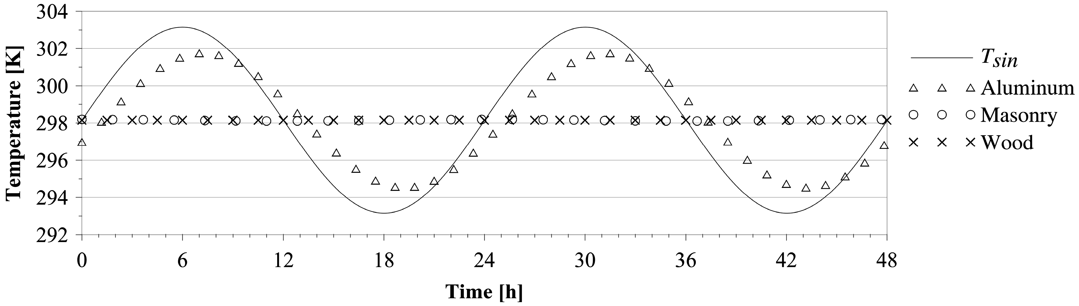
The solid body has been assumed isotropic and homogeneous. The material of the solid is the aluminum, which is characterized by: ρ = 2719 kg/m³, c_p = 871 J/(kgK), λ = 202.4 W/(mK).

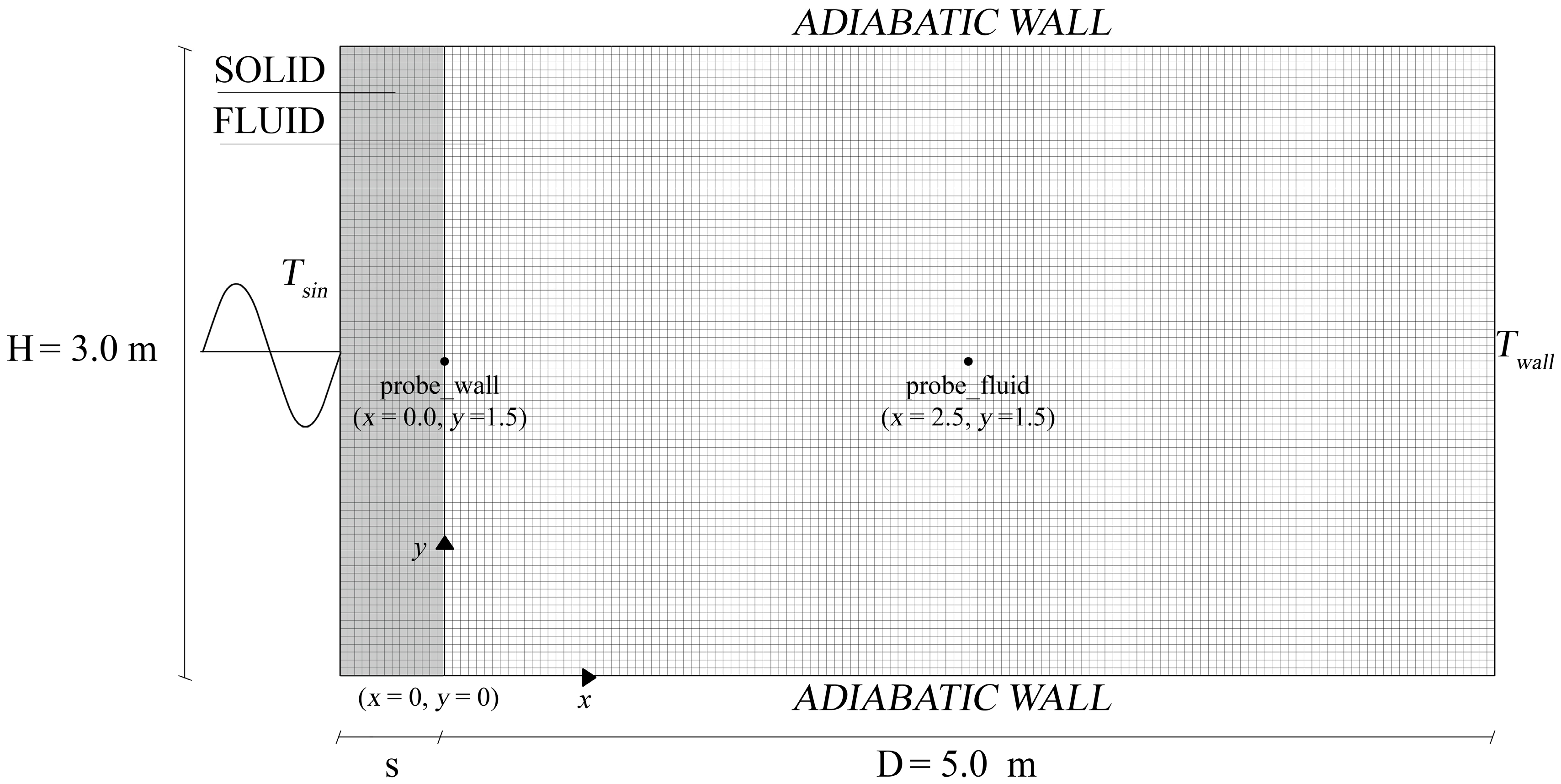
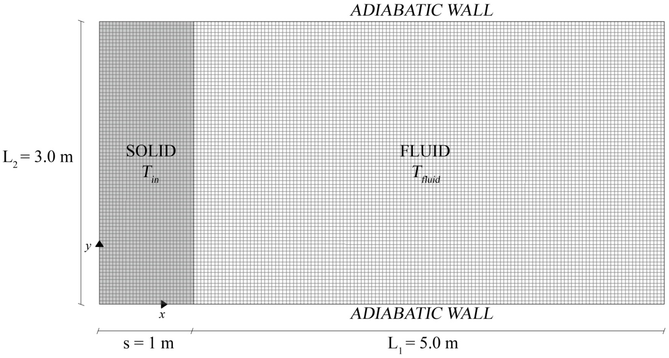
The geometry of Case A is represented by a rectangular domain having dimensions of L₁ = 5.0 m and L₂ = 3.0 m (Figure 2). A time-dependent sinusoidal temperature T_sin has been applied on one sidewall in the normal x direction, which follows the analytical Equation (1), where T_m = 298.15 K, Θ₀ = 5 K and ω = 7.3 × 10⁻⁵ rad/s.

A fixed temperature T_wall = 298.15 K has been applied on the opposite sidewall, while the top and the bottom walls have been considered as adiabatic.

Since the geometry is very simple, a mesh with a structured grid, composed by 10,500 cells (interval size 0.035 m), has been chosen for the discretization.

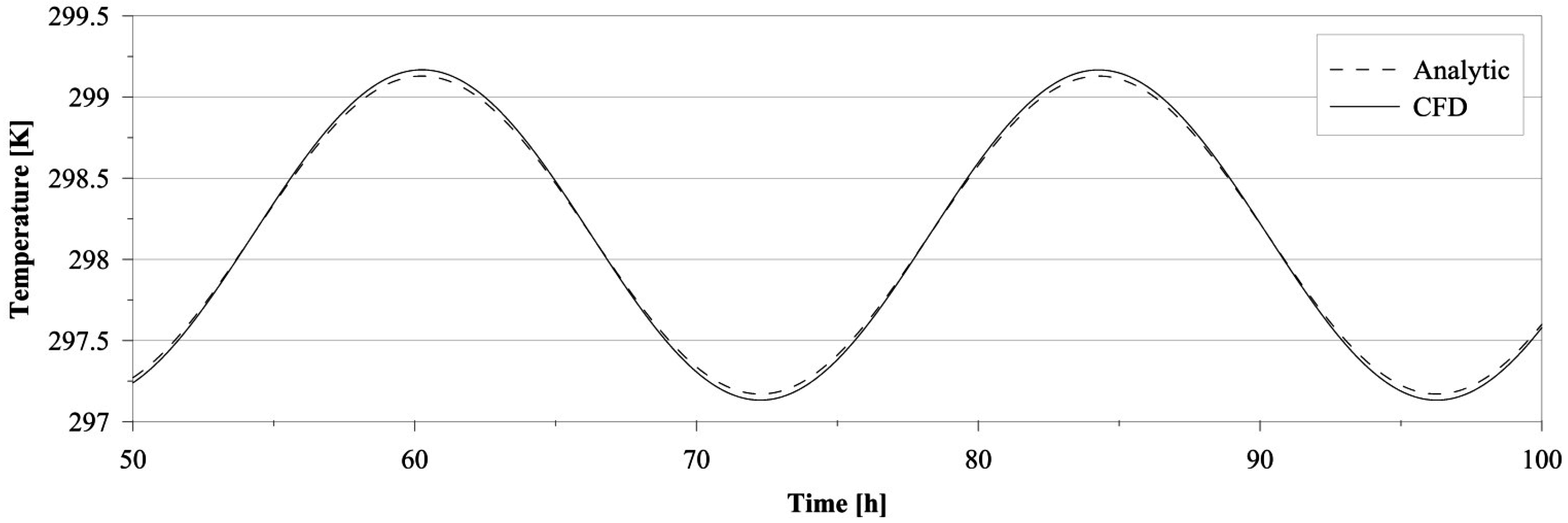
Figure 3 shows the temperature trends in the center of the solid domain (x = 2.5 m, y = 1.5 m) in both numerical and analytical analyses. The analytical data are derived (2).

The results show that the two temperatures have the same trends and almost the same values. The comparison between analytical and numerical data has been performed also through the root mean square error (RMSE) in a time period of 24 h after the stabilization of the simulation. The obtained RMSE value is 0.027 K. Therefore, CFD simulations can be considered accurate enough for the analysis of the transient heat conduction through a solid.

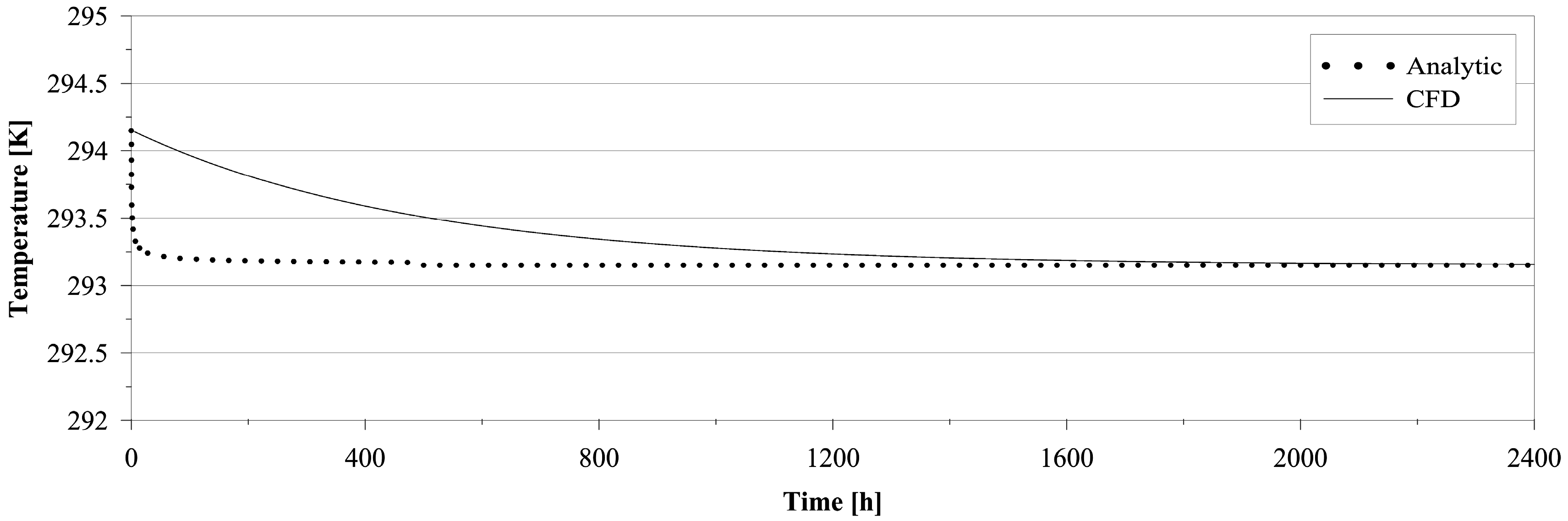
The geometry of Case B is represented by a solid domain with a rectangular shape and a thickness of s = 1 m, while the fluid domain dimensions are L₁ = 5.0 m and L₂ = 3.0 m (Figure 4). The heat exchange coefficient has been imposed equal to 10 W/(m²K). The temperature of the fluid domain has been kept constant and equal to T_fluid = 293.15 K, while the solid temperature T_in has been left free to evolve, starting from a temperature of 215.15 K. The top and the bottom walls have been considered adiabatic.

As the previous case, the geometry is very simple. For this reason, a mesh with a structured grid, composed by 12,700 cells (interval size 0.035 m), has been chosen for the discretization.

Figure 5 shows the temperature trends in the center of the solid domain (x = 0.5 m, y = 1.5 m) in both numerical and analytical analyses. In this case, it is possible to use the Equation (5), where λ, α, h, and T_∞ are assumed constant. The assumption of constant h and T is almost never encountered in real cases, as for the one-dimensional application.

Analytical and numerical temperature trends greatly differ only before the stabilization of the simulation (around 2000 h). The root mean square error (RMSE) has been evaluated in a time period of 400 h after 2000 h of simulated time and the obtained value is 0.0001 K. It is possible to assume that the numerical model approximates accurately the analytical one also in this case.

The CFD model has been considered validated, accepting that the obtained values are affected by a minimum error. Therefore, it has been applied to a similar real model where a solid envelope adjacent to the flow domains is subject to thermal sinusoidal boundary conditions varying with time.

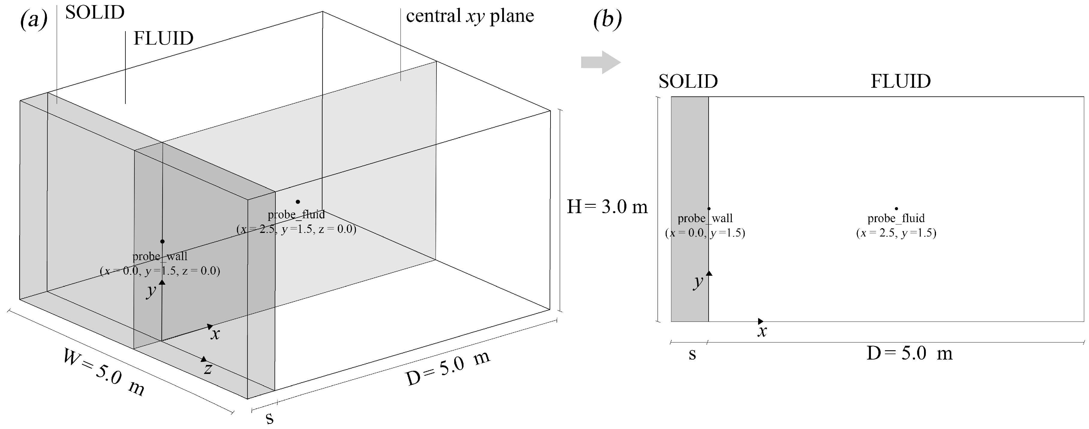
4. 3D-2D Simplification

The periodic stabilized regime has been numerically applied to a model of a simple closed room with a rectangular plan of 5 × 5 m (W × D) and H = 3 m. The room model is influenced by an outdoor thermal forcing applied on a solid wall, while the opposite wall is adjacent to an environment at a fixed temperature. The other walls have been considered adjacent to environments having the same temperature of the room; therefore, it has been possible to assume that there is not heat transfer through those walls (adiabatic process).

The 3D geometry of the room has been simplified in a 2D computational domain representing the longitudinal section on the central xy plane (Figure 6).

In this work, this simplification has been possible since the considered room has a preferential symmetry plan along the z axis. The choice of a 2D model allows lower computational costs without compromising the accuracy of the results.

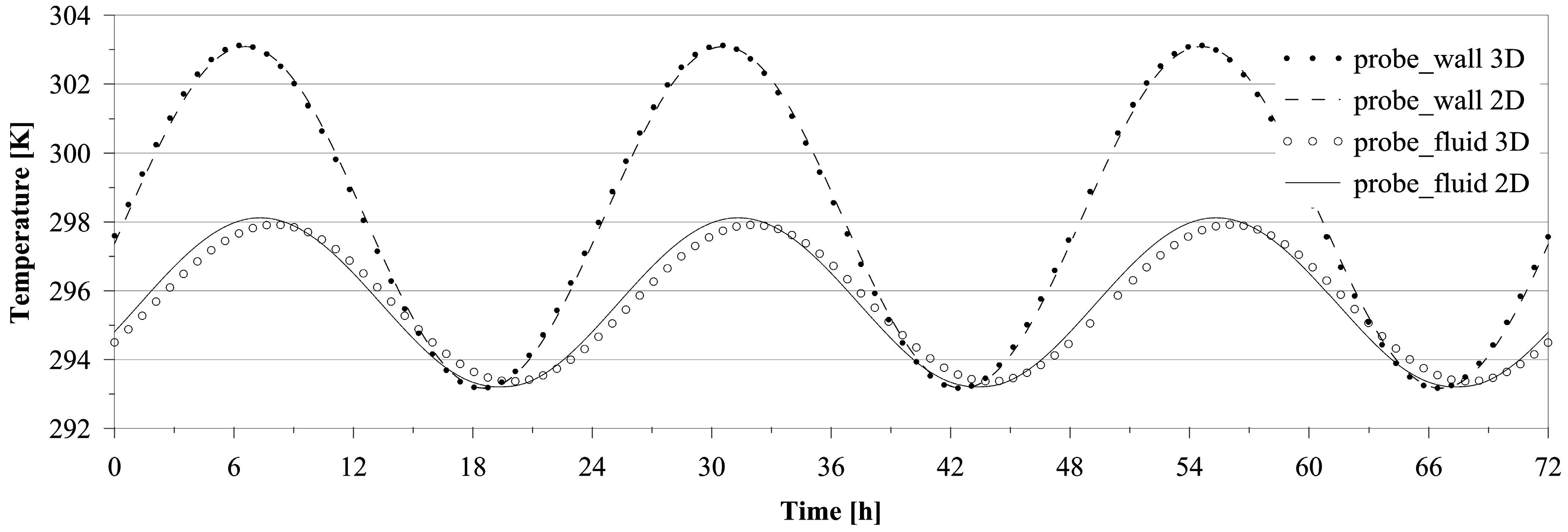
In order to demonstrate the effectiveness of this choice, both the 3D and 2D models have been simulated with the same boundary conditions and simulation settings. The results have been shown in terms of temperature trends at the end of the solid domain (probe_wall) and in the center of the fluid domain (probe_fluid) and in terms of contours of the velocity magnitude in the central plane xy (Figure 6).

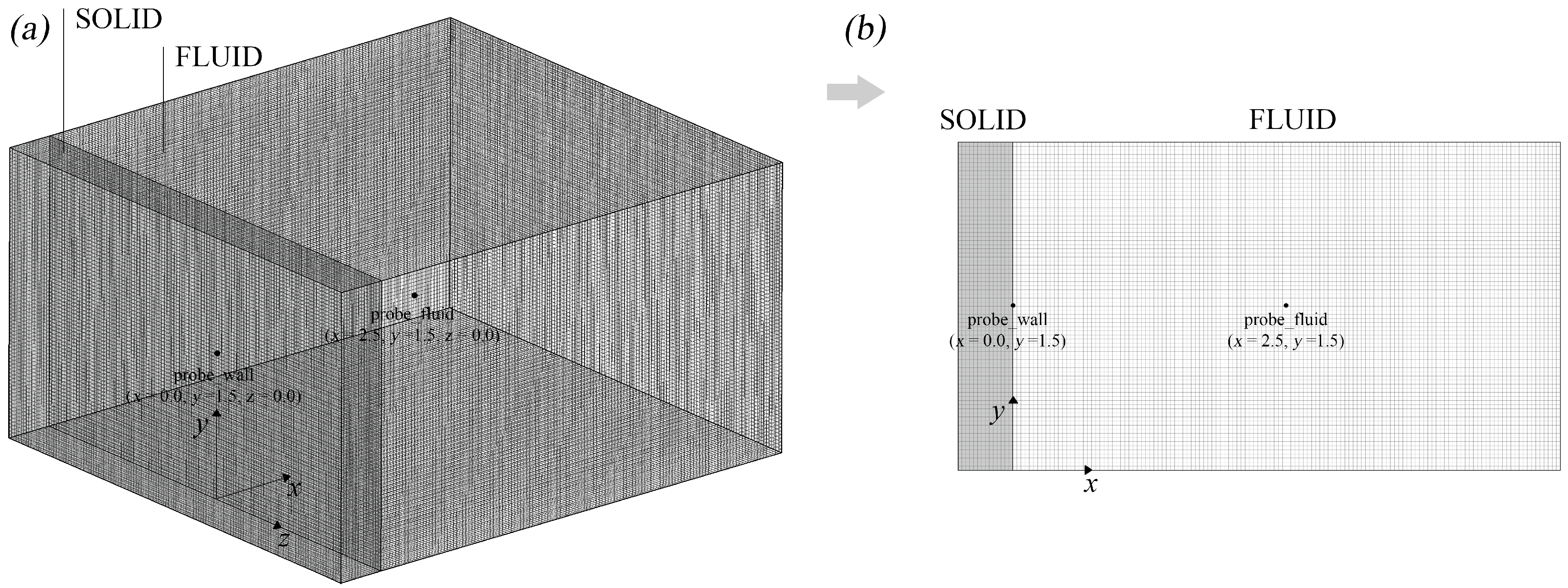
The two computational models have been discretized using an orthogonal grid (Figure 7).

A grid independence test has been performed for the 2D model in order to demonstrate the independence of the results from the mesh spacing. A fixed temperature has been applied on the external wall of the solid domain and the static temperature in the middle of the fluid domain (probe_fluid) has been chosen as a parameter for the test. Assuming the finest mesh considered, Mesh D (mesh spacing equal to 0.0175 m), as the pivot case, it is possible to observe that the differences percentage Δ% with the other three meshes are always very low (

Table 2. Mesh sensitivity test for the 2D model.

	Mesh A	Mesh B	Mesh C	Mesh D
Cells of the mesh	116,80	2920	730	46,720
Interval size	0.035	0.07	0.14	0.0175
Δ%	0.02%	0.17%	0.30%	-

). The mesh with the lower error, Mesh A (mesh spacing equal to 0.035 m), has been used for these CFD analyses and the 3D model has been discretized considering the same interval size of the mesh, with an amount of 155,344 cells.

Both models are composed by two computational domains, one for the solid wall and one for the fluid inside the room. The same boundary conditions have been taken into account (Figure 8). A time-dependent sinusoidal temperature T_sin has been applied on the external surface of the solid domain following the analytical Equation (1), while a fixed temperature T_wall has been applied on the right sidewall of the fluid domain. The top and the bottom walls have been considered adiabatic assuming those surfaces adjacent to environments at the same temperature, as usually happens in a room of a building. Also, the other two sides of the 3D model have been considered adiabatic. Neither a fixed temperature nor a convection coefficient have been applied to the indoor environment. Therefore, the temperature is free to evolve under the influence of the external temperature.

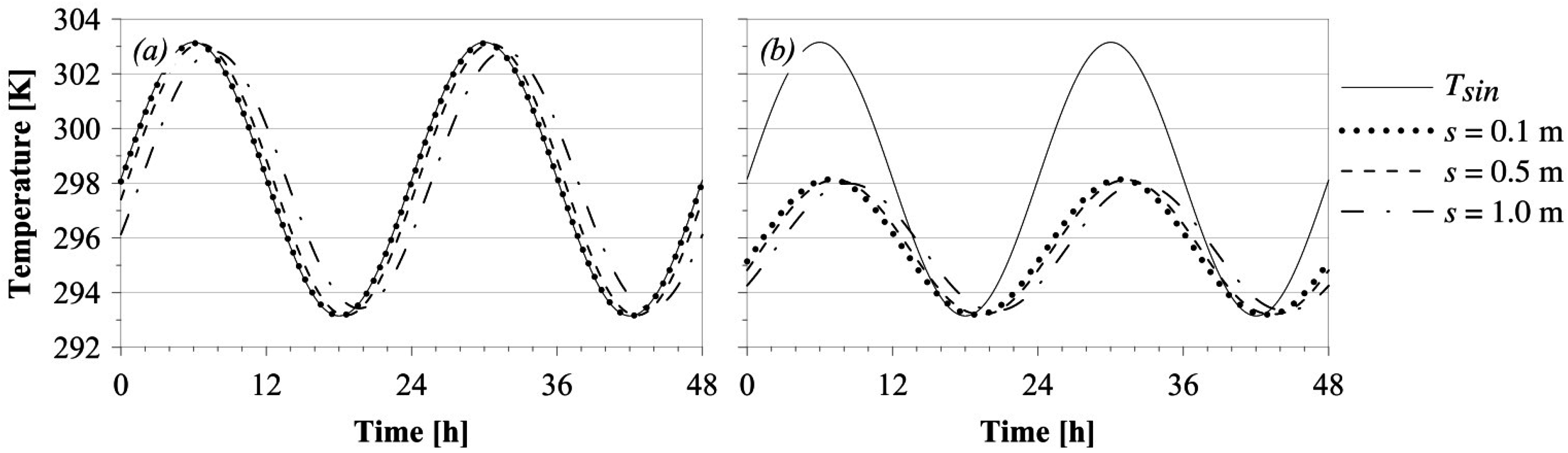
Figure 9 shows the temperature trends in probe_wall and probe_fluid for the two models.

The results show that the temperatures have almost the same values and trends. The root mean square error (RMSE) is 0.2 K for probe_fluid and 0.1 K for probe_wall. Therefore, it is possible to assume that the values obtained from the 2D numerical model describe the thermal phenomena with the same accuracy of the 3D model.

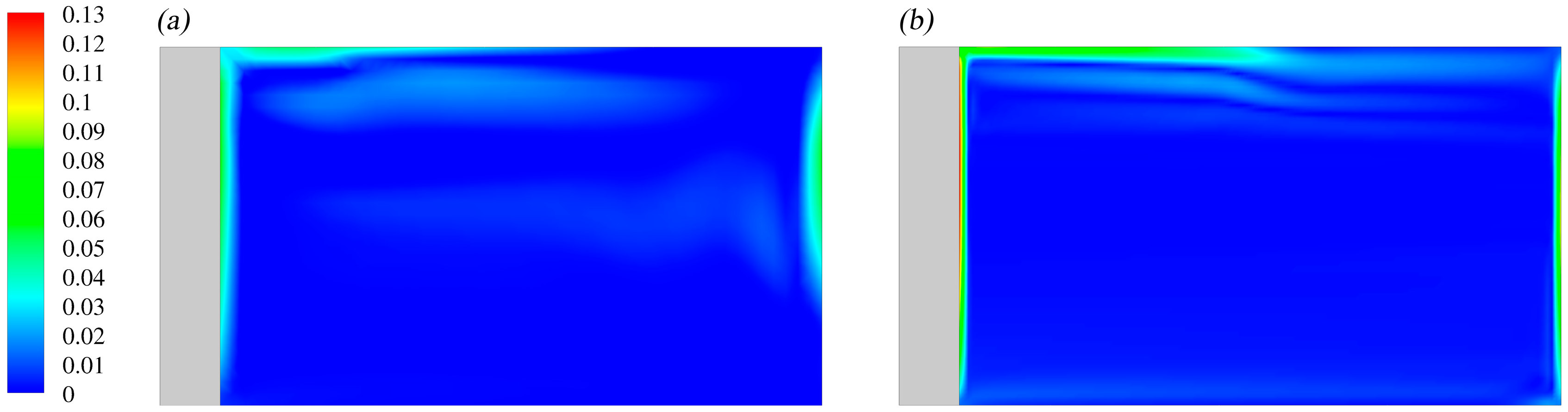
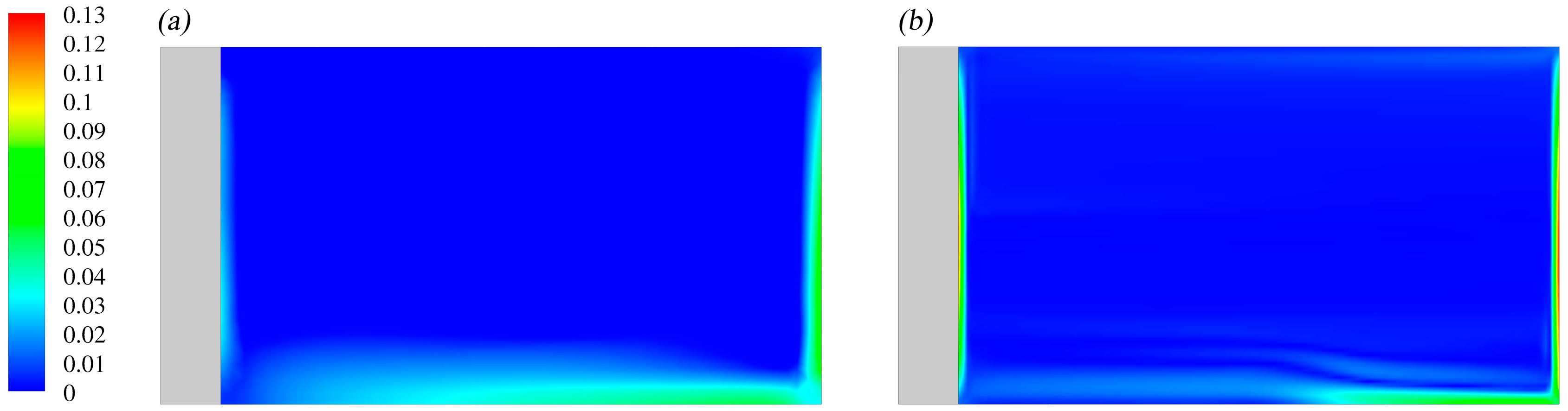
This assumption has been supported also by the analysis of the fluid field and the convective motions (Figure 10 and Figure 11).

The air motions have been analyzed in two different time steps which represent the highest and the lowest peaks of the sinusoidal temperature T_sin. The results are almost the same for the two models. The fluid fields show in both time steps two areas characterized by an acceleration of the air. The most noticeable difference between the two models is the air velocity of the acceleration zones, which reaches highest values in the 2D model. This phenomenon is due to an increase of kinetic energy in the 2D model, where the air motions are distributed only in two directions. However, these differences have been considered small enough to be ignored. Therefore, the two models show comparable results also from a fluid dynamic point of view.

5. Analytical Evaluation of the Solid Envelope

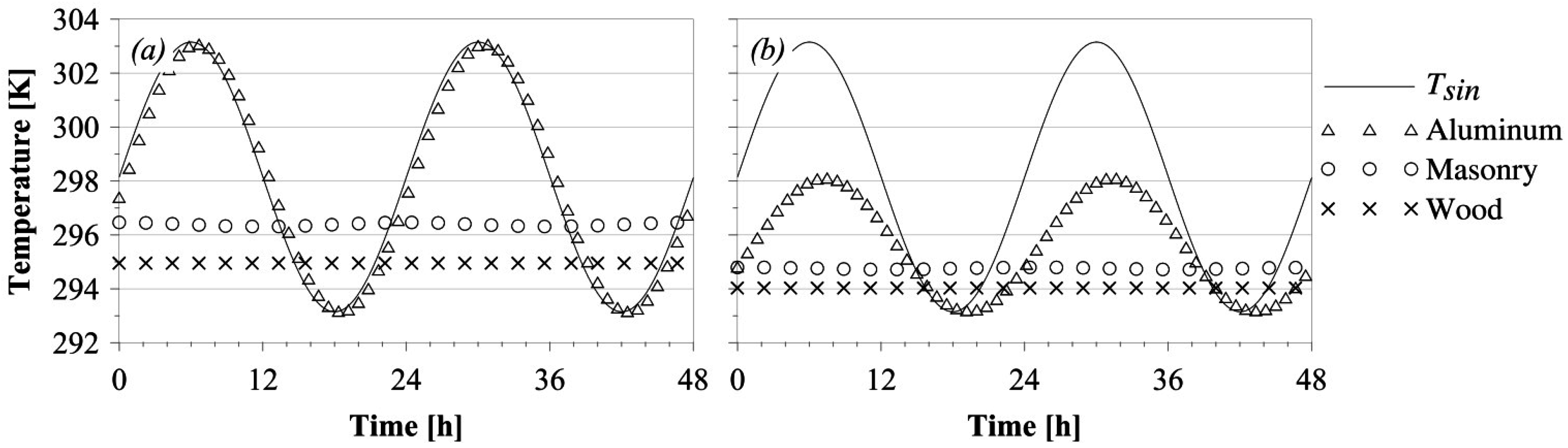
The analysis of building materials and building elements is a crucial aspect in the evaluation of the effects of outdoor microclimatic conditions on indoor environment. For this reason, the temperature trends at the end of the different analyzed walls have been analytically calculated considering a semi-infinite solid and applying Equation (2). This calculation has been performed for the walls in Case 1 and Case 2 in order to compare the variation between an ideal geometry and a more realistic one. In both cases, a sinusoidal temperature T_sin given by the Equation (1), where T_m = 298.15 K, Θ₀ = 5 K and ω = 7.3 × 10⁻⁵ rad/s, has been applied on the sidewall of the solid domain.

Three different materials have been taken into account: aluminum, masonry and wood. Thermo-physical properties of the materials (density, specific heat capacity, conductivity) have been derived from UNI 10351:1994 [39] and UNI EN ISO 10456:2007 [40] (

Table 3. Thermo-physical properties of the chosen materials.

	Aluminum	Masonry	Wood
ρ	2719	1700	700
λ	202.4	0.58	0.17
cp	871	850	2310

).

These materials have been chosen because of their different capability in transmitting, damping and delaying a thermal input. Considering a fixed thickness of the solid wall s = 0.5 m, the properties of the wall vary as shown in

Table 4. Thermo-physical properties of the solid wall as the material changes.

	Aluminum	Masonry	Wood
U	5.80	0.97	0.33
σ	72.18	0.86	0.01
τr	1.25	18.18	35.22
ϴ	3.61	0.04	0.00

.

The temperature trends at the end of the wall have been shown in Figure 12 for the three considered materials.

Another important aspect that influences the thermal behavior of the building envelope is the thickness of the building elements. Three different thicknesses s of the solid domain have been taken into account (0.1 m, 0.5 m and 1.0 m), while the material has been set as aluminum (Table 3). The thermo-physical properties of the solid wall vary as shown in

Table 5. Thermo-physical properties of the solid wall as the thicknesses changes.

	s = 0.1 m	s = 0.5 m	s = 1.0 m
U	5.86	5.80	5.71
σ	93.69	72.18	52.09
τr	0.25	1.25	2.49
ϴ	4.68	3.61	2.60

.

The temperature trends at the end of the wall for the three considered thicknesses s are shown in Figure 13.

The reported analytical data underline how and to what extent the external temperature is perceived on the internal surface of the wall in the semi-infinite solid case. Knowing Θ₀ and the thermal damping factor σ of each building element, it has been possible to calculate the semi-amplitude of the sinusoidal wave applied on the external surface once it is perceived on the internal surface.

The solid wall of aluminum delays and damps a little the temperature T_sin and it is possible to expect that indoor temperature largely follows the sinusoidal trend of the outdoor thermal forcing. On the contrary, the solid walls composed by masonry and wood greatly impact on the outdoor temperature. For this reason, it is perceived almost as a constant temperature. In the same way, the higher the thickness s is, the less the indoor temperature varies following the external sinusoidal trend.

6. CFD Results: Sensitivity Analysis for Different Geometrical Parameters and Boundary Conditions

6.1. Materials Sensitivity Test

The materials described in Table 3 have been used for the solid wall of Case 1. The sinusoidal temperature T_sin described in the previous chapter has been applied on the external side of the solid wall; the temperature of the right wall of the fluid environment is T_wall = 293.15 K, while the top and the bottom walls have been set adiabatic.

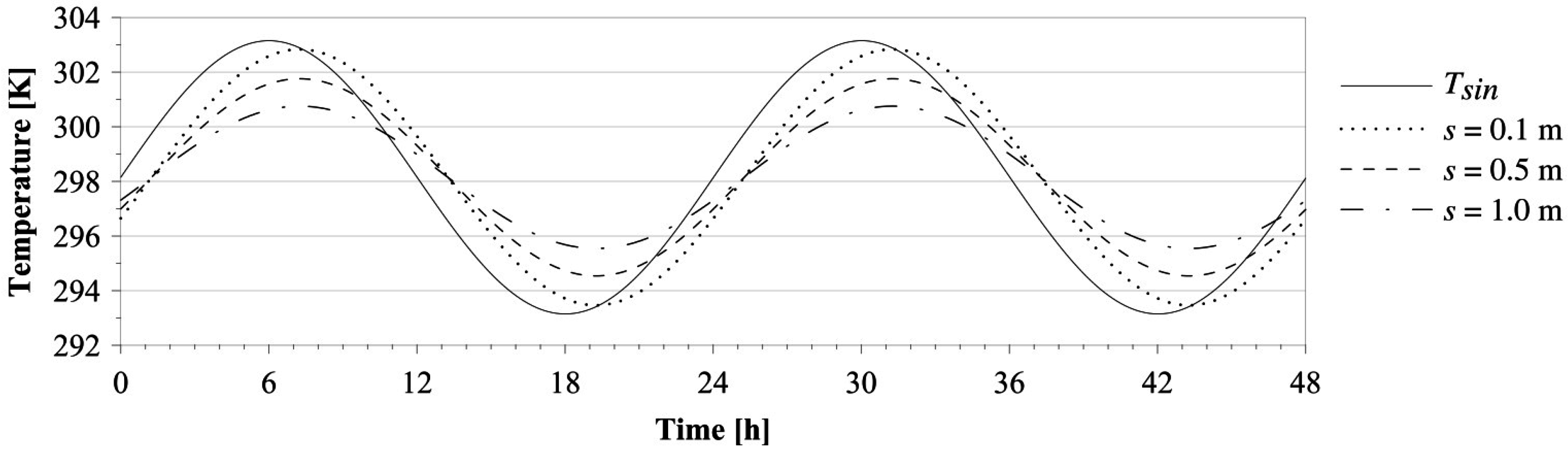
Figure 14 shows the temperature trends at the end of the wall and in the center of the fluid domain for different solid wall materials compared with the external sinusoidal temperature.

The numerical results confirm the analytical data shown in Table 3 and Table 4, underlining the relationship between thermo-physical properties of building materials and architectural elements.

The characteristics of the sinusoidal wave at the end of the wall and in the center of the fluid domain have been derived from the numerical results and analyzed in-depth in

Table 6. Case 1: Characteristics of the sinusoidal wave in probe_wall and probe_fluid.

		Aluminum		Masonry		Wood
	Tsin	probe_wall	probe_fluid	probe_wall	probe_fluid	probe_wall	probe_fluid
σ	-	99.15	49.14	1.52	0.76	0.01	0.01
τr	-	0.55	1.23	18.05	18.60	31.14	31.26
ϴ	5.0	4.96	2.46	0.08	0.04	0.00	0.00
Tm	298.10	298.13	295.67	296.39	294.76	294.96	294.04

.

As expected, the semi-amplitude ϴ of the thermal wave decreases between x = 0.0 m and x = 2.5 m. This decrement is easily shown in the aluminum and the masonry cases, while it is very slight in the wood wall.

After passing through the masonry and wood walls, the sinusoidal wave is almost totally damped. On the contrary, in the case of the aluminum, the fluid environment damps the sinusoidal wave more than the wall. In this case, the thermal wave T_sin quickly passes through the solid domain and it is subject to a small damping, because of the high thermal conductivity of the material. Therefore, the resulting thermal wave dissipates a great part of its energy in the fluid environment, which is characterized by a lower thermal conductivity. For the other two materials, T_sin arrives into the fluid environment with almost completely lowered oscillations.

This behavior is noticeable also in the variation of T_m for the three materials, which decreases with the decrease of the thermal conductivity. Higher energy levels correspond to higher T_m, as it happens for aluminum.

Finally, regarding the phase lag, masonry and wood have similar behavior. The phase lag, indeed, remains almost the same between the end of the wall and the center of the fluid domain in both cases. On the contrary, the phase lag increases for aluminum. This phenomenon is probably due to the influence of T_sin on the indoor environment. In the cases where masonry and wood have been used, the entering temperature is almost constant and has almost the same values. Therefore, it is easy to suppose that the fluid field is almost the same. In the aluminum case, indeed, the great oscillation of the entering temperature causes different fluid motions, which take to different thermo-fluid dynamic behavior.

The comparison between the numerical results in probe_wall and the analytical data (Table 4 and Figure 12) shows how the fluid environment is able to limit the energy losses from the solid wall. In the comparison with the analytical results, the phase lag is lower and the thermal damping factor and the semi-amplitude are higher in the numerical simulations. This phenomenon is emphasized by the decrease of the thermal conductivity of the material, which is related to a lower energy level dissipated by the wall and, consequently, to lower heat levels transferred to the fluid environment. This suggests that the analytical solution for the semi-infinite solid is too approximated for the case of a wall adjacent to a fluid environment.

6.2. Thickness Sensitivity Test

Three different wall thicknesses s have been modeled in Case 2. The applied thermal boundary conditions are the same used in Case 1, while the material has been set as aluminum (Table 3); this choice has been made since the other two materials greatly damp and delay the external sinusoidal wave, approximating it to a constant temperature. For this reason, the indoor thermal variations are too small to be perceived. The obtained temperature trends are shown in Figure 15.

The characteristics of the sinusoidal wave at the end of the wall and in the center of the fluid domain have been derived from the numerical results (

Table 7. Case 2: Characteristics of the sinusoidal wave in probe_wall and probe_fluid.

		s = 0.1 m		s = 0.5 m		s = 1.0 m
	Tsin	probe_wall	probe_fluid	probe_wall	probe_fluid	probe_wall	probe_fluid
σ	-	99.66	49.41	99.15	49.14	93.84	46.45
τr	-	0.04	0.74	0.55	1.23	1.66	2.43
ϴ	5	4.98	2.47	4.96	2.46	4.69	2.32
Tm	298.15	298.13	295.67	298.13	295.67	298.12	295.66

).

Comparing the numerical results and the analytical data (Table 5 and Figure 13), the trend of thermal damping factor at thickness variation is the most evident phenomenon. Based on the analytical data, the sinusoidal wave is expected to be highly damped with the increase of thickness. Despite that, the thermal damping factor is almost the same in the numerical results in both probe_wall (90%–100%) and probe_fluid (45%–50%). Furthermore, unlike Case 1, the numerical values of phase lag in the same point of the wall are higher than the analytical ones, and this difference is emphasized consequently to the increase of the thicknesses s, passing from an increase of thermal lag of 6% (s = 0.1 m) to 80% (s = 1.0 m). On the contrary, thermal damping factor and semi-amplitude are lower compared to the analytical ones. Also in this case, the difference increases with the increase of thickness s. These differences are caused by the convective phenomena in the fluid environment, which are not taken into account in the analytical calculation.

The numerical results also suggest that the higher the thickness is, the lower the energy levels of the entering wave are. This phenomenon causes lower heat exchanges among the fluid particles of the enclosure, damping less the temperature. On the contrary, basing on the same assumption, a lower thickness allows higher energy levels of the entering wave and a consequent higher heat exchange and a higher damping of the temperature.

Also in this case, it is possible to assume that the analytical solution for the semi-infinite solid is too approximated for the case of a wall adjacent to a fluid environment.

6.3. External Sinusoidal Temperature T_sin Sensitivity Test

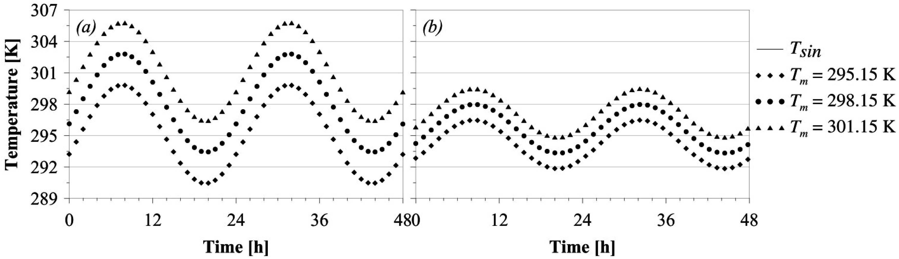
The third and fourth sensitivity analyses concern the variation of the thermal boundary conditions, while the thermo-physical properties of the solid wall have been left unaltered. In the third case the sinusoidal wave T_sin applied on the external surface of the solid wall has been changed varying the initial T_m,0, while Θ₀ = 5 K and ω = 7.3 × 10⁻⁵ rad/s have been left unaltered in all the simulations. Three T_m,0 have been considered: 295.15 K, 298.15 K and 301.15 K. The temperature on the right wall of the fluid environment is T_wall = 293.15 K, while the top and the bottom walls have been set adiabatic. The material has been set as aluminum (Table 3) and the thickness of the wall s is equal to 1.0 m.

The obtained temperature trends are shown in Figure 16.

The characteristics of the sinusoidal wave at the end of the wall and in the center of the fluid domain have been derived from the numerical results (

Table 8. Case 3: Characteristics of the sinusoidal wave in probe_wall and probe_fluid.

		Tm,0 = 295.15		Tm,0 = 298.15		Tm,0 = 301.15
	Tsin	probe_wall	probe_fluid	probe_wall	probe_fluid	probe_wall	probe_fluid
σ	-	93.86	46.29	93.84	46.45	93.84	46.48
τr	-	1.59	2.35	1.66	2.43	1.59	2.36
ϴ	5	4.69	2.32	4.69	2.32	4.69	2.32
Tm	298.15	295.14	294.17	298.12	295.66	301.10	297.17

).

Varying T_m,0 of the sinusoidal wave T_sin, the temperature trends in probe_wall and probe_fluid are damped and delayed in the same way, since the thermo-physical properties of the building materials and elements are the same. The only noticeable difference is the variation of T_m which increases with the T_m,0 of the external temperature. Furthermore, T_m does not increase proportionally to T_m,0 since it is influenced also by T_wall. The results underline an interesting relation applicable in the analyzed case: the temperature T_m of the environment can be calculated, as the average between the external T_m,0 and the fixed T_wall basing on the distance from the considered walls. This phenomenon is not computable when the analytical solution is applied.

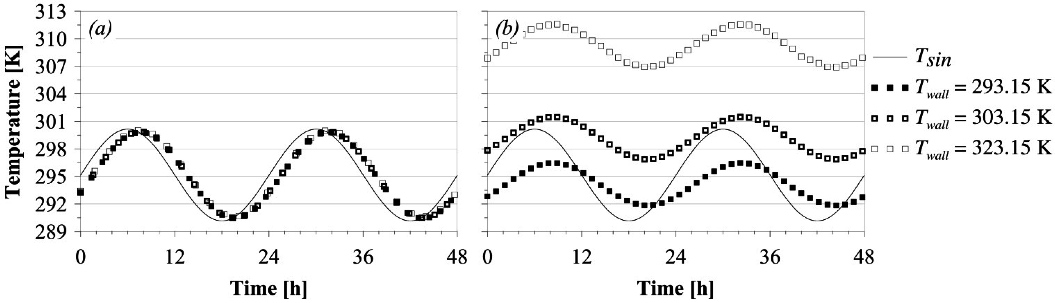
6.4. External Fixed Temperature T_wall Sensitivity Test

Finally, the influence of the temperature T_wall on the interior environment has been investigated. Thermo-physical properties of materials and building elements are the same as Case 3, while the sinusoidal temperature T_sin follows Equation (2), where T_m = 295.15 K, Θ₀ = 5 K and ω = 7.3 × 10⁻⁵ rad/s. Three T_wall have been considered: 293.15 K, 303.15 K and 323.15 K.

The obtained temperature trends are shown in Figure 17.

The characteristics of the sinusoidal wave at the end of the wall and in the center of the fluid domain have been derived from the numerical results (

Table 9. Case 4: Characteristics of the sinusoidal wave in probe_wall and probe_fluid.

		Twall = 293.15 K		Twall = 303.15 K		Twall = 323.15 K
	Tsin	probe_wall	probe_fluid	probe_wall	probe_fluid	probe_wall	probe_fluid
σ	-	93.86	46.29	93.84	45.99	93.83	51.02
τr	-	1.59	2.35	1.60	2.40	1.61	2.24
ϴ	5	4.69	2.31	4.69	2.30	4.69	2.55
Tm	298.15	295.14	294.17	295.20	299.19	295.32	309.20

).

The results show the same physical phenomena observed in Case 3. The indoor temperatures, indeed, are characterized by the same thermal damping factors and phase lags, and their T_m is function of the average temperature of T_sin and T_wall.

This consideration is helpful when materials with low thermal damping factors and high phase lags are taken into account (such as the previously analyzed wood and masonry). In that case, indeed, the external sinusoidal temperature is perceived inside as a constant temperature equal to T_m and the indoor temperature is equal to the average of the all the external temperatures considered. As for the previous cases, this phenomenon is not computable when the analytical solution is applied.

7. Conclusions

The indoor microclimate of buildings is influenced by several parameters. Especially when the indoor conditions are subject to an outdoor transient thermal forcing and they are free to evolve in a periodic stabilized regime, the heat transfer phenomena are very complex. For this reason, several studies use some simplifications in the investigation of these physical problems. To the best of our knowledge, an exact solution to solve this phenomenon does not exist also from the analytical point of view. The aim of this research is to propose a first approach to solving the thermal phenomena inside environments where the temperature is free to evolve, such as buildings not equipped with HVAC systems.

The coupling of conduction and convection inside a simplified room has been investigated through Computational Fluid Dynamics. Different preliminary analyses have been taken into account in order to validate the numerical results and to evaluate possible discrepancies between the 3D geometry of the room and its simplification in a 2D numerical model. The numerical model has been studied taking into account four configurations and performing parametric analysis in order to understand the response of the indoor environment when thermal inputs and thermo-physical properties of the envelope change.

In the first and the second configurations (Case 1 and Case 2), the thermo-physical properties of the solid domain have been varied considering three different construction materials (aluminum, masonry and wood) and three different thicknesses of the wall (0.1 m, 0.5 m and 1 m.) The results of these analyses underline a strong dependence of the indoor temperature on thermo-physical properties of the solid envelope. Furthermore, the entering thermal wave is also greatly influenced by the energy exchanges with the fluid particles in the indoor environment. These heat exchanges are shown in terms of decrease of the thermal damping factor related to the variation of thermal conductivity.

In the third and fourth sensitivity analyses (Cases 3 and Case 4), the thermal boundary conditions have been varied considering three T_m,0 of the sinusoidal temperature (295.15 K, 298.15 K and 301.15 K) and three different T_wall (293.15 K, 303.15 K and 323.15 K). In these cases, the results underline that the thermal damping factor and the phase lag do not change with these variations, while the T_m in the middle of the fluid environment (probe_fluid) changes proportionally to the average of T_m,0 and T_wall.

The comparison between the obtained numerical data and the analytical ones for the four cases have shown that the case of the semi-infinite solid is too approximate to correctly describe the temperature trend inside a fluid environment adjacent to a wall in a periodic stabilized regime. More in detail, the analytical calculation does not take into account the convective phenomena in the fluid environment resulting from the heat levels exchanged with the wall. This situation is clear when the thermo-physical characteristics of the solid vary, especially in Case 2, where the phase lag and thermal damping factor do not change as expected from the analytical calculations. For this reason, further developments of the research are needed in order to formulate more accurate predictions of the periodic stabilized regime.

This work is a first step to better understanding these physical phenomena and it would lay the groundwork to develop analytical correlations to predict the trend of the temperature inside an environment free from thermal control and subject only to the varying external thermal conditions.