Land Use Change Impact on Flooding Areas: The Case Study of Cervaro Basin (Italy)

 ,
,  , , and
Abstract
:1. Introduction
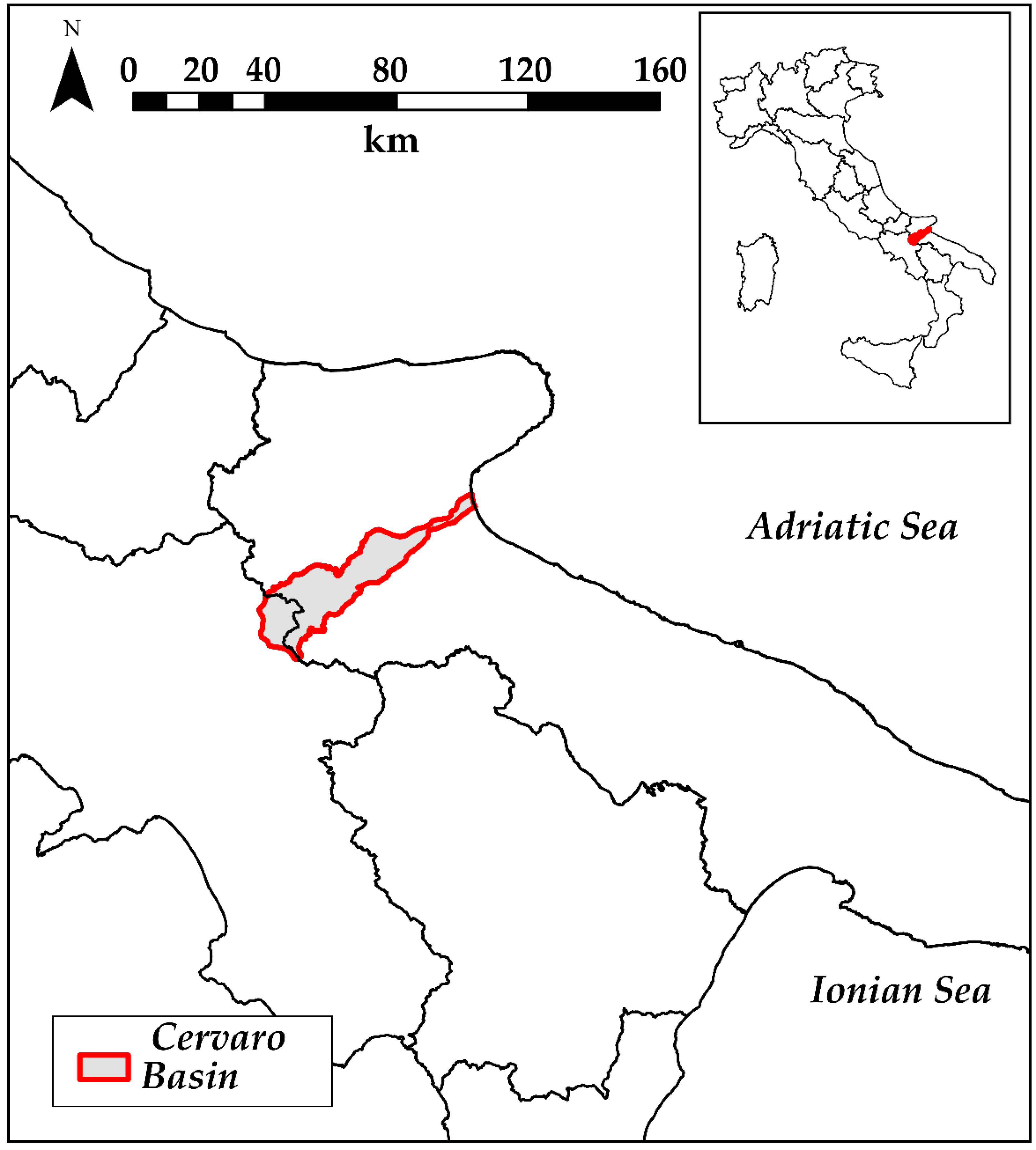
2. The Study Area
3. Data and Methods
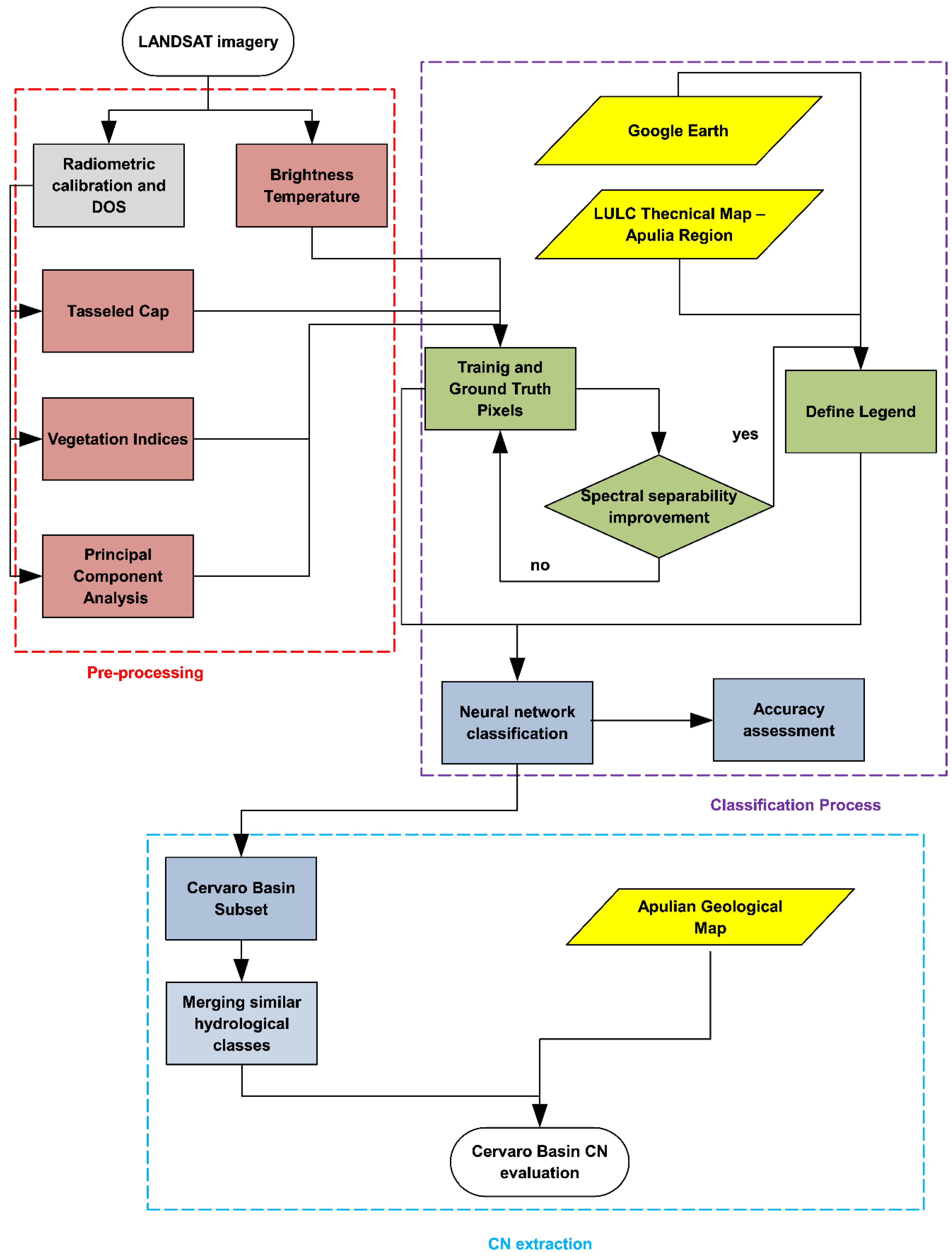
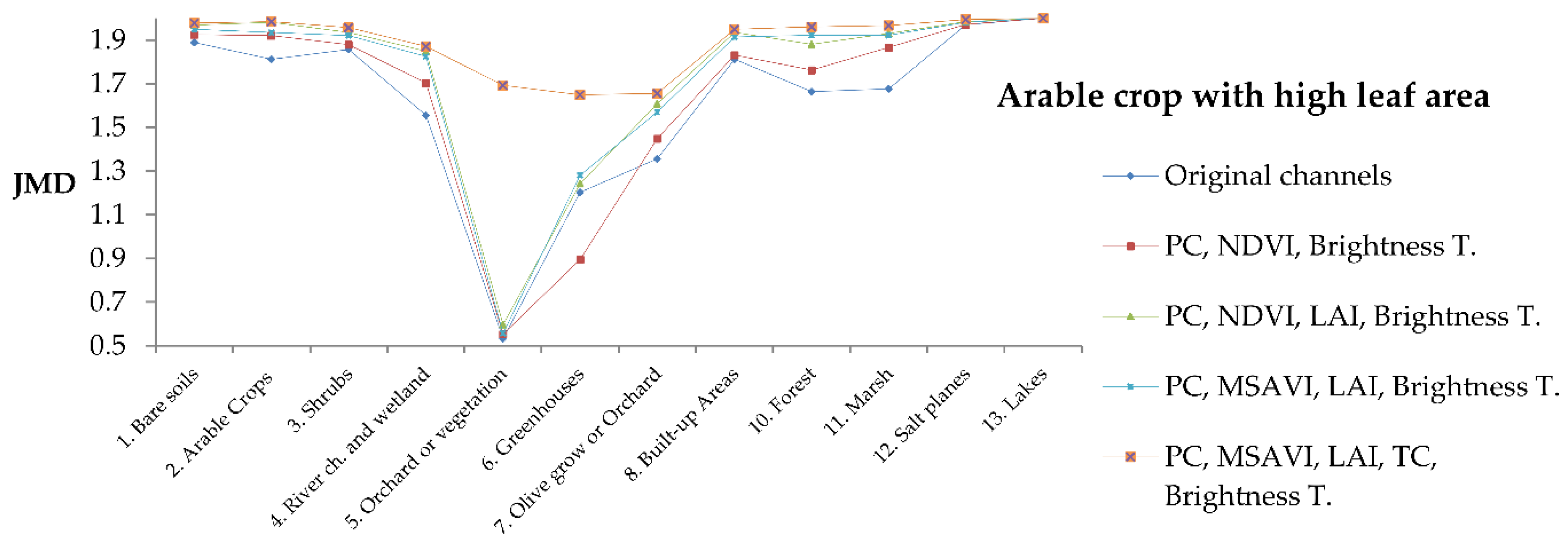
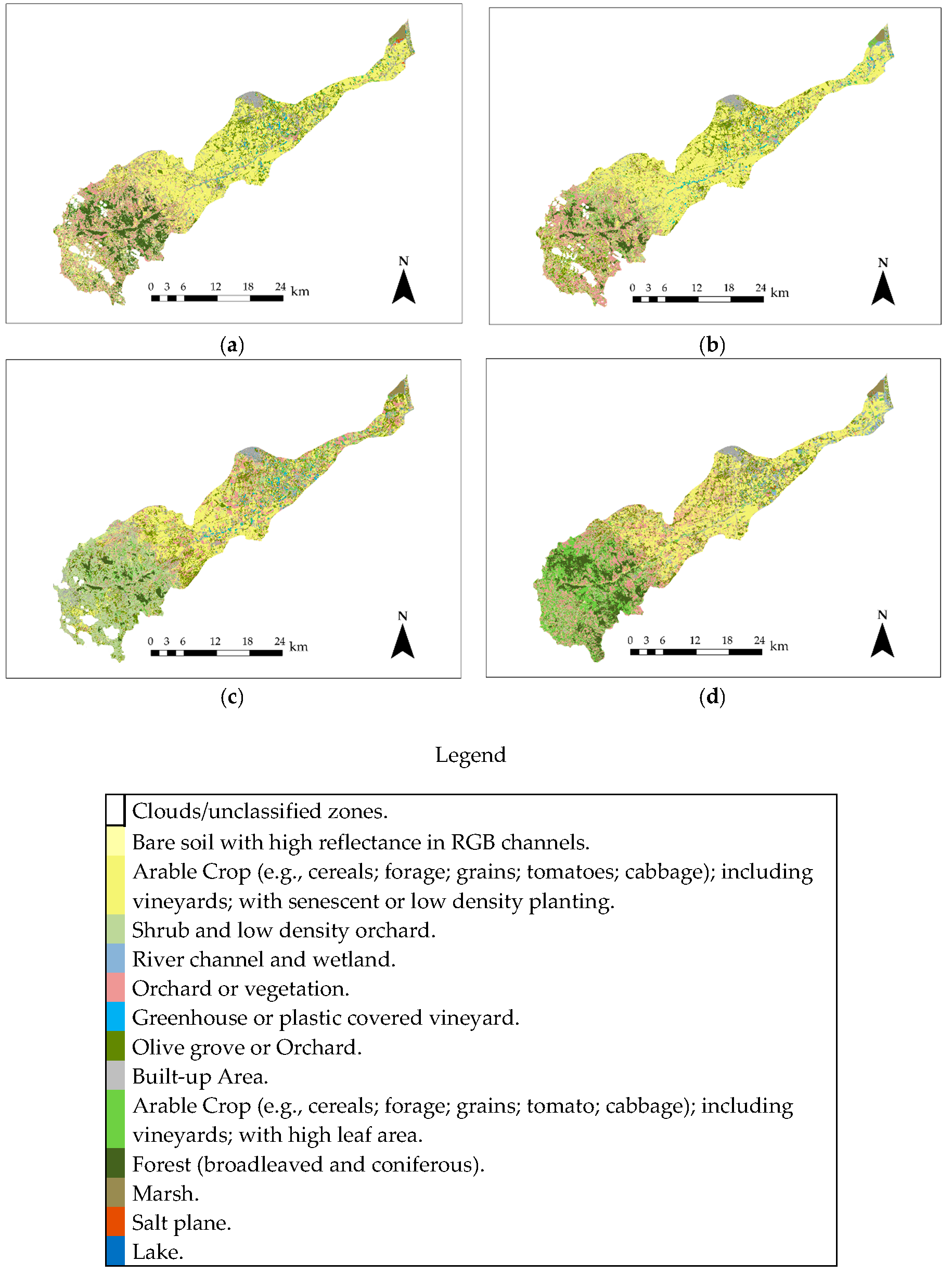
3.1. LANDSAT Data Processing
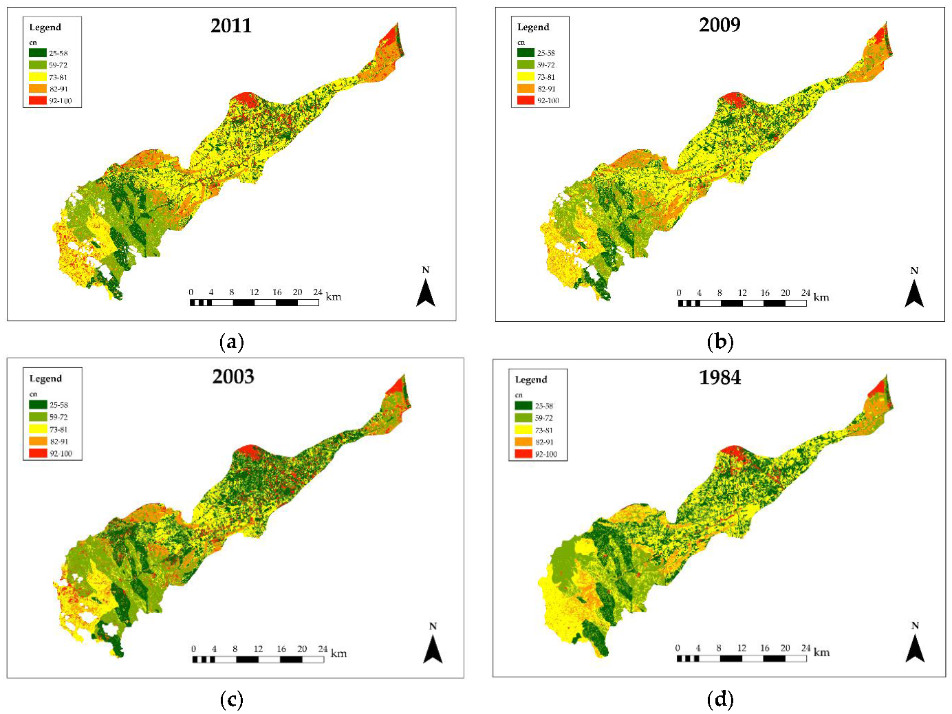
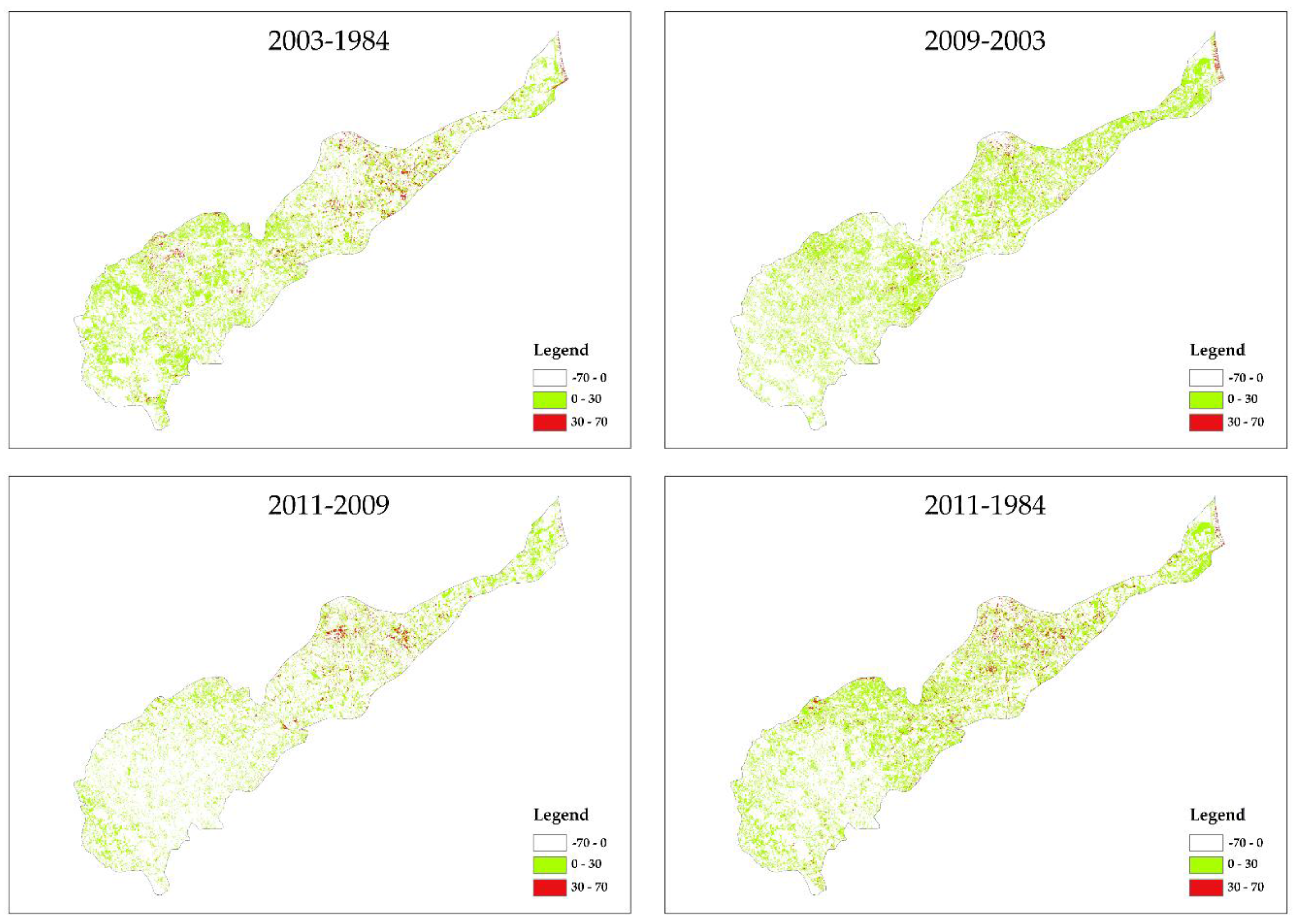
3.2. Curve Number Extraction
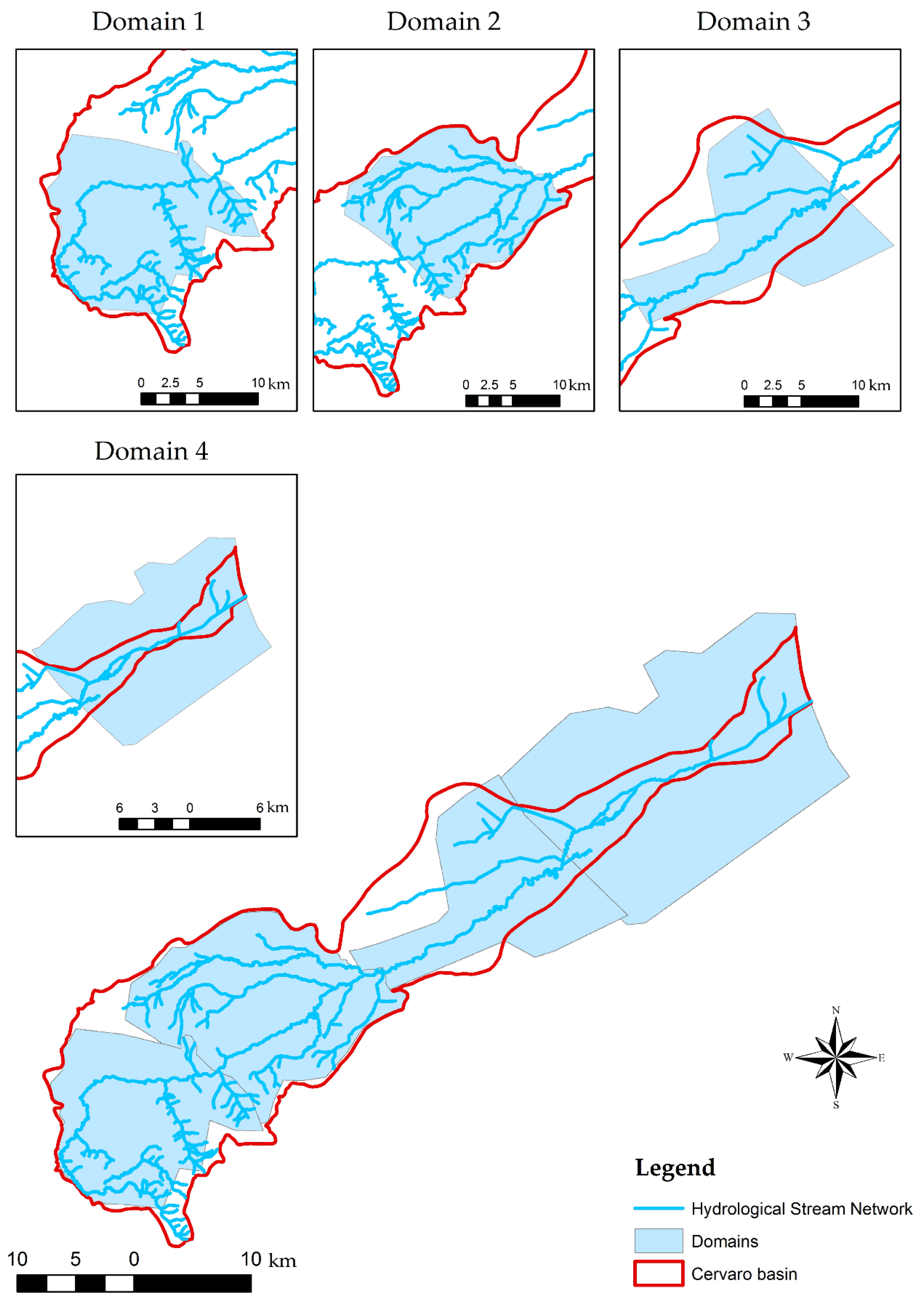
3.3. Hydrologic Modeling
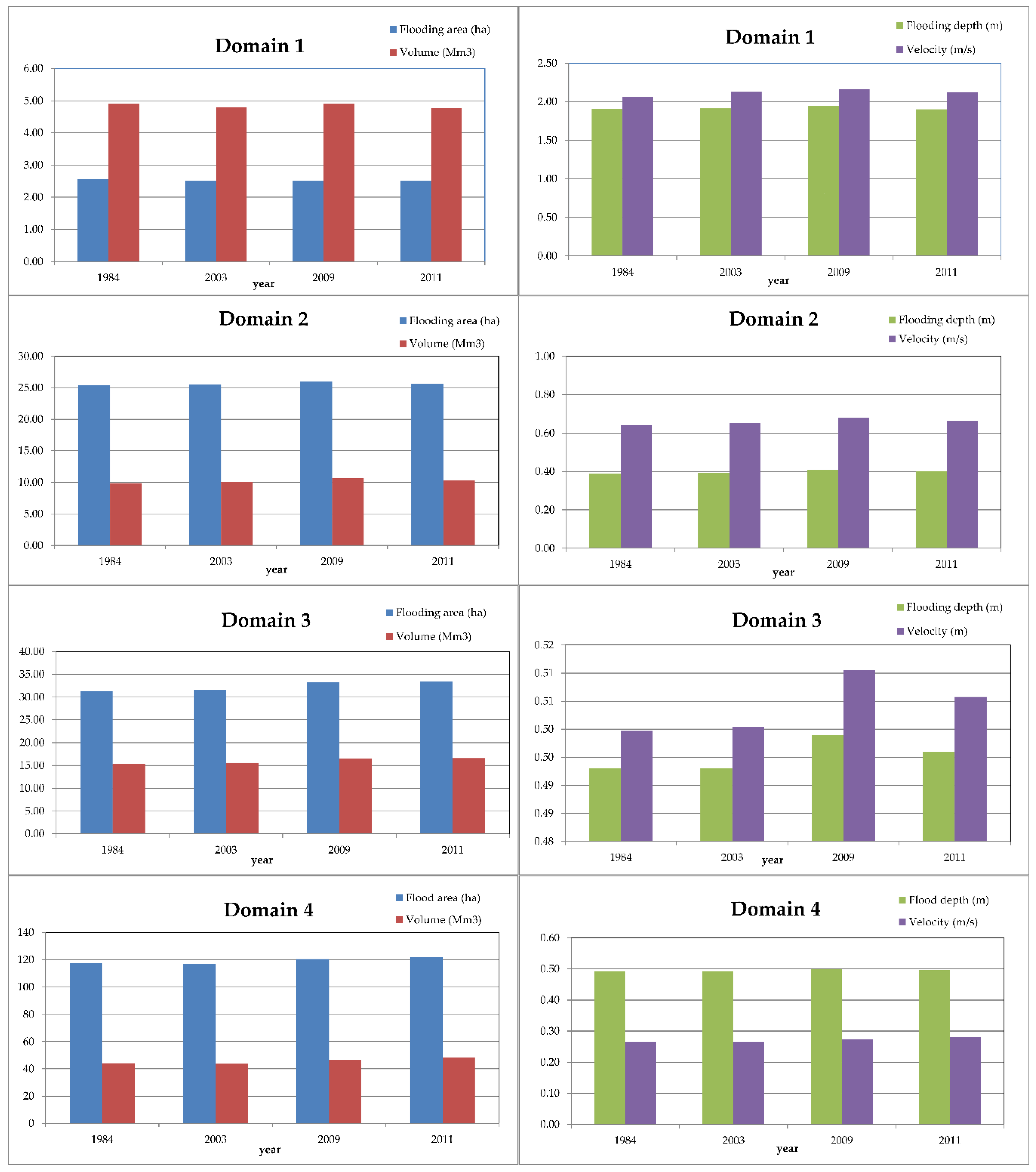
4. Results
5. Conclusions
Author Contributions
Conflicts of Interest
References
- Di Palma, F.; Amato, F.; Nolè, G.; Martellozzo, F.; Murgante, B. A SMAP Supervised Classification of Landsat Images for Urban Sprawl Evaluation. ISPRS Int. J. Geo-Inf. 2016, 5, 109. [Google Scholar] [CrossRef]
- Olang, L.; Fürst, J. Effects of land cover change on flood peak discharges and runoff volumes: Model estimates for the Nyando River Basin, Kenya. Hydrol. Process. 2011, 25, 80–89. [Google Scholar] [CrossRef]
- Olang, L.O.; Kundu, P.; Bauer, T.; Fürst, J. Analysis of spatio-temporal land cover changes for hydrological impact assessment within the Nyando River Basin of Kenya. Environ. Monit. Assess. 2011, 179, 389–401. [Google Scholar] [CrossRef] [PubMed]
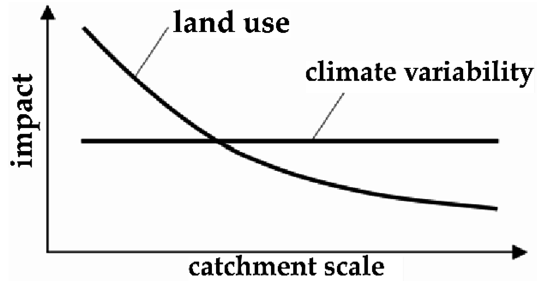
- Blöschl, G.; Ardoin-Bardin, S.; Bonell, M.; Dorninger, M.; Goodrich, D.; Gutknecht, D.; Matamoros, D.; Merz, B.; Shand, P.; Szolgay, J. At what scales do climate variability and land cover change impact on flooding and low flows? Hydrol. Process. 2007, 21, 1241–1247. [Google Scholar] [CrossRef]
- Pattison, I.; Lane, S.N. The link between land-use management and fluvial flood risk: A chaotic conception? Prog. Phys. Geogr. 2011, 36, 72–92. [Google Scholar] [CrossRef] [Green Version]
- Novelli, A.; Tarantino, E.; Caradonna, G.; Apollonio, C.; Balacco, G.; Piccinni, F. Improving the ANN Classification Accuracy of Landsat Data Through Spectral Indices and Linear Transformations (PCA and TCT) Aimed at LU/LC Monitoring of a River Basin. In Proceedings of the 16th International Conference on Computational Science and Its Applications, Beijing, China, 4–7 July 2016; Gervasi, O., Murgante, B., Misra, S., Rocha, A.M.A.C., Torre, C.M., Taniar, D., Apduhan, B.O., Stankova, E., Wang, S., Eds.; Springer: Beijing, China, 2016; pp. 420–432. [Google Scholar]
- Rejani, R.; Rao, K.; Osman, M.; Rao, C.S.; Reddy, K.S.; Chary, G.; Samuel, J. Spatial and temporal estimation of soil loss for the sustainable management of a wet semi-arid watershed cluster. Environ. Monit. Assess. 2016, 188, 1–16. [Google Scholar] [CrossRef] [PubMed]
- Gangodagamage, C.; Aggarwal, S. Integrating Satellite based Remote Sensing Observations with SCS Curve Number Method for Simplified Hydrologic Modeling in Ungauged Basins. Asian J. Geoinform. 2012, 12, 29–33. [Google Scholar]
- Gao, H.; Liu, J.; Eneji, A.E.; Han, L.; Tan, L. Using Modified Remote Sensing Imagery to Interpret Changes in Cultivated Land under Saline-Alkali Conditions. Sustainability 2016, 8, 619. [Google Scholar] [CrossRef]
- Rakwatin, P.; Sansena, T.; Marjang, N.; Rungsipanich, A. Using multi-temporal remote-sensing data to estimate 2011 flood area and volume over Chao Phraya River basin, Thailand. Remote Sens. Lett. 2013, 4, 243–250. [Google Scholar] [CrossRef]
- Zhan, X.; Sohlberg, R.; Townshend, J.; DiMiceli, C.; Carroll, M.; Eastman, J.; Hansen, M.; DeFries, R. Detection of land cover changes using MODIS 250 m data. Remote Sens. Environ. 2002, 83, 336–350. [Google Scholar] [CrossRef]
- Van der Sande, C.J.; De Jong, S.M.; De Roo, A.P.J. A segmentation and classification approach of IKONOS-2 imagery for land cover mapping to assist flood risk and flood damage assessment. Int. J. Appl. Earth Obs. Geoinf. 2003, 4, 217–229. [Google Scholar] [CrossRef]
- Panahi, A.; Alijani, B.; Mohammadi, H. The effect of the land use/cover changes on the floods of the Madarsu Basin of Northeastern Iran. J. Water Resour. Prot. 2010, 2, 373–379. [Google Scholar] [CrossRef]
- Descheemaeker, K.; Nyssen, J.; Poesen, J.; Raes, D.; Haile, M.; Muys, B.; Deckers, S. Runoff on slopes with restoring vegetation: A case study from the Tigray highlands, Ethiopia. J. Hydrol. 2006, 331, 219–241. [Google Scholar] [CrossRef]
- Gholami, V.; Jokar, E.; Azodi, M.; Zabardast, H.; Bashirgonbad, M. The influence of anthropogenic activities on intensifying runoff generation and flood hazard in Kasilian watershed. J. Appl. Sci. 2009, 9, 3723–3730. [Google Scholar]
- Lane, S.N.; Morris, J.; O’Connell, P.E.; Quinn, P.F. 18 Managing the rural landscape. In Future Flooding Coastal Erosion Risks; Thorne, C.R., Evans, E.P., Penning-Rowsell, E.C., Eds.; Thomas Telford Lt: London, UK, 2007; p. 297. [Google Scholar]
- Chen, X.; Tian, C.; Meng, X.; Xu, Q.; Cui, G.; Zhang, Q.; Xiang, L. Analyzing the effect of urbanization on flood characteristics at catchment levels. Proc. IAHS 2015, 370, 33–38. [Google Scholar] [CrossRef]
- Giordano, R.; D’Agostino, D.; Apollonio, C.; Scardigno, A.; Pagano, A.; Portoghese, I.; Lamaddalena, N.; Piccinni, A.F.; Vurro, M. Evaluating acceptability of groundwater protection measures under different agricultural policies. Agric. Water Manag. 2015, 147, 54–66. [Google Scholar] [CrossRef]
- Sivapalan, M.; Takeuchi, K.; Franks, S.; Gupta, V.; Karambiri, H.; Lakshmi, V.; Liang, X.; McDonnell, J.; Mendiondo, E.; O‘connell, P. IAHS Decade on Predictions in Ungauged Basins (PUB), 2003–2012: Shaping an exciting future for the hydrological sciences. Hydrol. Sci. J. 2003, 48, 857–880. [Google Scholar] [CrossRef]
- Giordano, R.; Milella, P.; Portoghese, I.; Vurro, M.; Apollonio, C.; D'Agostino, D.; Lamaddalena, N.; Scardigno, A.; Piccinni, A. An innovative monitoring system for sustainable management of groundwater resources: Objectives, stakeholder acceptability and implementation strategy. In Proceedings of Environmental Energy and Structural Monitoring Systems (EESMS), 2010 IEEE Workshop, Taranto, Italy, 9 September 2010; pp. 32–37.
- Sdao, F.; Merenda, L. Eventi alluvionali e fenomeni di piena verificatisi dal 1921 al 1985 in Puglia settentrionale. In Valutazione Delle Piene in Puglia; Copertino, V.A., Fiorentino, M., Eds.; CNR-GNDCI: Potenza, Italy, 1992; pp. 57–80. [Google Scholar]
- NERC. Flood Studies Report; Centre for Ecology and Hydrology: Wallingford, UK, 1975. [Google Scholar]
- Feng, Q.; Gong, J.; Liu, J.; Li, Y. Monitoring Cropland Dynamics of the Yellow River Delta based on Multi-Temporal Landsat Imagery over 1986 to 2015. Sustainability 2015, 7, 14834–14858. [Google Scholar] [CrossRef]
- Lausch, A.; Pause, M.; Doktor, D.; Preidl, S.; Schulz, K. Monitoring and assessing of landscape heterogeneity at different scales. Environ. Monit. Assess. 2013, 185, 9419–9434. [Google Scholar] [CrossRef] [PubMed]
- Niu, C.; Wang, Q.; Chen, J.; Zhang, W.; Xu, L.; Wang, K. Hazard Assessment of Debris Flows in the Reservoir Region of Wudongde Hydropower Station in China. Sustainability 2015, 7, 15099–15118. [Google Scholar] [CrossRef]
- Xu, D.; Fu, M. Detection and modeling of vegetation phenology spatiotemporal characteristics in the middle part of the Huai river region in China. Sustainability 2015, 7, 2841–2857. [Google Scholar] [CrossRef]
- Nolè, G.; Lasaponara, R.; Lanorte, A.; Murgante, B. Quantifying Urban Sprawl with Spatial Autocorrelation Techniques using Multi-Temporal Satellite Data. IJAEIS 2014, 5, 19–37. [Google Scholar] [CrossRef]
- Sehgal, S. Remotely sensed LANDSAT image classification using neural network approaches. Int. J. Eng. Res. Appl. 2012, 2, 43–46. [Google Scholar]
- Tarantino, E.; Novelli, A.; Aquilino, M.; Figorito, B.; Fratino, U. Comparing the MLC and JavaNNS Approaches in Classifying Multi-Temporal LANDSAT Satellite Imagery over an Ephemeral River Area. IJAEIS 2015, 6, 83–102. [Google Scholar] [CrossRef]
- Xu, H. Extraction of urban built-up land features from Landsat imagery using a thematicoriented index combination technique. Photogramm Eng. Remote Sens. 2007, 73, 1381–1391. [Google Scholar] [CrossRef]
- Patel, N.; Mukherjee, R. Extraction of impervious features from spectral indices using artificial neural network. Arab. J. Geosci. J. 2015, 8, 3729–3741. [Google Scholar] [CrossRef]
- Pepe, M.; Prezioso, G. A Matlab Geodetic Software for Processing Airborne LIDAR Bathymetry Data. Int. Arch. Photogram Remote Sens. Spatial Inf. Sci. 2015, 40, 167. [Google Scholar] [CrossRef]
- Pepe, M.; Prezioso, G. Two approaches for dense DSM generation from aerial digital oblique camera system. In Proceedings of the 2nd International Conference on Geographical Information Systems Theory, Applications and Management, Rome, Italy, 26–27 April 2016; pp. 63–70.
- Chander, G.; Markham, B. Revised Landsat-5 TM radiometric calibration procedures and postcalibration dynamic ranges. IEEE Trans. Geosci. Remote 2003, 41, 2674–2677. [Google Scholar] [CrossRef]
- Hadjimitsis, D.G.; Clayton, C.; Retalis, A. On the darkest pixel atmospheric correction algorithm: A revised procedure applied over satellite remotely sensed images intended for environmental applications. In Proceedings of the SPIE-The International Society for Optical Engineering, Barcelona, Spain, 9–12 September 2003; Volume 5239. p. 465.
- Aquilino, M.; Novelli, A.; Tarantino, E.; Iacobellis, V.; Gentile, F. Evaluating the potential of GeoEye data in retrieving LAI at watershed scale. In Proceedings of SPIE-The International Society for Optical Engineering, Amsterdam, Netherland, 22–25 September 2014; p. 92392B.
- Balacco, G.; Figorito, B.; Tarantino, E.; Gioia, A.; Iacobellis, V. Space-time LAI variability in Northern Puglia (Italy) from SPOT VGT data. Environ. Monit. Assess. 2015, 187, 1–15. [Google Scholar] [CrossRef] [PubMed]
- Gao, F.; Anderson, M.C.; Kustas, W.P.; Houborg, R. Retrieving leaf area index from landsat using MODIS LAI products and field measurements. IEEE Geosci. Remote SENS. Lett. 2014, 11, 773–777. [Google Scholar]
- Manfreda, S.; Fiorentino, M.; Iacobellis, V. DREAM: A distributed model for runoff, evapotranspiration, and antecedent soil moisture simulation. Adv. Geosci. 2005, 2, 31–39. [Google Scholar] [CrossRef]
- Novelli, A.; Tarantino, E.; Fratino, U.; Iacobellis, V.; Romano, G.; Gentile, F. A data fusion algorithm based on the Kalman filter to estimate leaf area index evolution in durum wheat by using field measurements and MODIS surface reflectance data. Remote Sens. Lett. 2016, 7, 476–484. [Google Scholar] [CrossRef]
- Tarantino, E.; Novelli, A.; Laterza, M.; Gioia, A. Testing high spatial resolution WorldView-2 imagery for retrieving the leaf area index. In Proceedings of Third International Conference on Remote Sensing and Geoinformation of the Environment, Paphos, Cyprus, 16–19 March 2015; p. 95351N.
- Qi, J.; Chehbouni, A.; Huete, A.; Kerr, Y.; Sorooshian, S. A modified soil adjusted vegetation index. Remote Sens. Environ. 1994, 48, 119–126. [Google Scholar] [CrossRef]
- Zhang, C.; Pan, Z.; Dong, H.; He, F.; Hu, X. Remote Estimation of Leaf Water Content Using Spectral Index Derived From Hyperspectral Data. In Proceedings of First International Conference on Information Science and Electronic Technology, Wuhan, China, 21–22 March 2015; pp. 20–24.
- Aguiar, A.; Shimabukuro, Y.; Mascarenhas, N. Use of synthetic bands derived from mixing models in the multispectral classification of remote sensing images. Int. J. Remote Sens. 1999, 20, 647–657. [Google Scholar] [CrossRef]
- Novelli, A.; Aguilar, M.A.; Nemmaoui, A.; Aguilar, F.J.; Tarantino, E. Performance evaluation of object based greenhouse detection from Sentinel-2 MSI and Landsat 8 OLI data: A case study from Almería (Spain). Int. J. Appl. Earth Obs. 2016, 52, 403–411. [Google Scholar] [CrossRef]
- Bruzzone, L.; Roli, F.; Serpico, S.B. An extension of the Jeffreys-Matusita distance to multiclass cases for feature selection. IEEE Trans. Geosci. Remote 1995, 33, 1318–1321. [Google Scholar] [CrossRef]
- Crist, E.P.; Laurin, R.; Cicone, R.C. Vegetation and soils information contained in transformed Thematic Mapper data. In Proceedings of the International Geoscience and Remote Sensing Symposium, Zürich, Switzerland, 8–11 September 1986; European Space Agency Publications: Paris, France, 1986; pp. 1465–1470. [Google Scholar]
- Canty, M.J. Image analysis, classification and change detection in remote sensing: with algorithms for ENVI/IDL and Python; Crc Press: Boca Raton, FL, USA, 2014. [Google Scholar]
- Ingram, J.C.; Dawson, T.P.; Whittaker, R.J. Mapping tropical forest structure in southeastern Madagascar using remote sensing and artificial neural networks. Remote Sens. Environ. 2005, 94, 491–507. [Google Scholar] [CrossRef]
- Jensen, J.; Qiu, F.; Ji, M. Predictive modelling of coniferous forest age using statistical and artificial neural network approaches applied to remote sensor data. Int. J. Remote Sens. 1999, 20, 2805–2822. [Google Scholar]
- Demuth, H.; Beale, M.; Hagan, M. Neural network toolbox TM 6 User’s guide. The MathWorks: Natick, MA, USA, 2008. [Google Scholar]
- Dorofki, M.; Elshafie, A.H.; Jaafar, O.; Karim, O.A.; Mastura, S. Comparison of artificial neural network transfer functions abilities to simulate extreme runoff data. In International Proceedings of Chemical, Biological and Environmental Engineering, Proceedings of 2012 International Proceedings of Chemical, Biological and Environmental Engineering, Kuala Lumpur, Malaysia, 5–6 May 2012; LACSIT Press: Singapore, 2012; pp. 39–44. [Google Scholar]
- NRCS. National Engineering Handbook: Part 630—Hydrology; Natural Resources Conservation Service: Washington, DC, USA, 2004.
- Deshmukh, D.S.; Chaube, U.C.; Hailu, A.E.; Gudeta, D.A.; Kassa, M.T. Estimation and comparision of curve numbers based on dynamic land use land cover change, observed rainfall-runoff data and land slope. J. Hydrol. 2013, 492, 89–101. [Google Scholar] [CrossRef]
- Kowalik, T.; Walega, A. Estimation of CN parameter for small agricultural watersheds using asymptotic functions. Water 2015, 7, 939–955. [Google Scholar] [CrossRef]
- INEA. Studio Sull’uso Irriguo Della Risorsa Idrica Nelle Regioni Obiettivo 1; INEA: Rome, Italy, 2001. [Google Scholar]
- Ferro, V. La Sistemazione dei Bacini Idrografici-Seconda Edizione; McGraw-Hill: Milano, Italy, 2006. [Google Scholar]
- Mishra, S.K.; Singh, V. Soil conservation Service Curve Number (SCS-CN) Methodology; Kluwer Academic Publishers: Dordrecht, Netherland, 2013; p. 42. [Google Scholar]
- Copertino, V.A.; Fiorentino, M. Valutazione Delle Piene in Puglia; Tipolitografia La Modernissima: Lamezia Terme, Italy, 1994. [Google Scholar]
- O’Brien, J. FLO-2D Users Manual; FLO-2D Inc.: Nutrioso, AR, USA, 2001. [Google Scholar]
- Piano Stralcio di Assetto Idrogeologico (PAI). Available online: http://www.adb.puglia.it (accessed on 15 December 2004).
- Veneziano, D.; Langousis, A. The areal reduction factor: A multifractal analysis. Water Resour. Res. 2005, 41, 1–15. [Google Scholar] [CrossRef]


| Date (mm/dd/yyyy) | ID | Sensor | Quality |
|---|---|---|---|
| 06/27/1984 | LT51890311984179XXX06 | TM | 9 |
| 07/18/2003 | LT51890312003199MTI03 | TM | 9 |
| 06/16/2009 | LT51890312009167MOR00 | TM | 9 |
| 06/22/2011 | LT51890312011173MOR00 | TM | 9 |
| Scene (date) | Overall Accuracy [%] |
|---|---|
| 06/22/2011 | 89 |
| 06/16/2009 | 88 |
| 07/18/2003 | 86 |
| 06/27/1984 | 79 |
| Classes | Soil Conservation Service (SCS) hydrological cover classes | Hydrological Condition |
|---|---|---|
| Bare soil with high reflectance in RGB channels | Fallow-Bare soil | |
| River channel and wetland; Marsh; Salt plane; Lake | Water surfaces | |
| Forest (broadleaved and coniferous) | Woods | Good |
| Greenhouse or plastic covered vineyards; Built-up Area | Impervious areas | |
| Arable Crop (e.g., cereals; forage; grains; tomatoes; cabbage); including vineyards; with high leaf area | Close-seeded or broadcast legumes or rotation meadow (straight row) | Good |
| Arable Crop (e.g., cereals; forage; grains; tomatoes; cabbage); including vineyards; with senescent or low-density planting | Close-seeded or broadcast legumes or rotation meadow (straight row) | Poor |
| Shrub and low-density orchard; Orchard or vegetation; Olive grove or Orchard | Meadow |
© 2016 by the authors; licensee MDPI, Basel, Switzerland. This article is an open access article distributed under the terms and conditions of the Creative Commons Attribution (CC-BY) license (http://creativecommons.org/licenses/by/4.0/).
Share and Cite
Apollonio, C.; Balacco, G.; Novelli, A.; Tarantino, E.; Piccinni, A.F. Land Use Change Impact on Flooding Areas: The Case Study of Cervaro Basin (Italy). Sustainability 2016, 8, 996. https://doi.org/10.3390/su8100996
Apollonio C, Balacco G, Novelli A, Tarantino E, Piccinni AF. Land Use Change Impact on Flooding Areas: The Case Study of Cervaro Basin (Italy). Sustainability. 2016; 8(10):996. https://doi.org/10.3390/su8100996
Chicago/Turabian StyleApollonio, Ciro, Gabriella Balacco, Antonio Novelli, Eufemia Tarantino, and Alberto Ferruccio Piccinni. 2016. "Land Use Change Impact on Flooding Areas: The Case Study of Cervaro Basin (Italy)" Sustainability 8, no. 10: 996. https://doi.org/10.3390/su8100996