Article

Production Patterns of Eagle Ford Shale Gas: Decline Curve Analysis Using 1084 Wells

1
School of Business Administration, China University of Petroleum (Beijing); Fuxue Road 18, Changping, Beijing 102249, China
2
Global Energy Systems, Department of Earth Sciences, Uppsala University; Villavägen 16, Uppsala 75236, Sweden
*
Author to whom correspondence should be addressed.
Sustainability 2016, 8(10), 973; https://doi.org/10.3390/su8100973
Submission received: 24 May 2016 / Revised: 14 September 2016 / Accepted: 14 September 2016 / Published: 27 September 2016
(This article belongs to the Section Energy Sustainability)

Abstract

:
This paper analyzes and quantifies characteristic production behavior using historical data from 1084 shale gas wells in the Eagle Ford shale play from 2010 to 2014. Decline curve analysis, using Hyperbolic and Stretched Exponential models, are used to derive average decline rates and other characteristic parameters for shale gas wells. Both Hyperbolic and Stretched Exponential models fit well to aggregated and individual well production data. The hyperbolic model is found to perform slightly better than the Stretched Exponential model in this study. In the Eagle Ford shale play, about 77% of wells reach the peak production of 1644–4932 mil cubic feet per day; the production decline rate of the first year is around 70%, and over the first two years it is around 80%; shale gas wells were estimated to yield estimated ultimate recoverable total resources of 1.41–2.03 billion cubic feet (20 years as life span), which is in line with other studies.

1. Introduction

Shale rocks can be defined as any laminated consolidated rock with >67% clay-sized materials and are typically formed in depositional environments where fine-grained particles fall out of suspension [1]. Significant amounts of organic material can become embedded in shales and allow them to generate hydrocarbons. However, extremely low matrix permeability (typically ranging from nD to μD) is a challenge for commercial exploitation. Extractable natural gas resources trapped in shale formations are called shale gas.
A report by the US Energy Information Administration (EIA), which covered 137 shale formations in 41 countries, estimated that the technically recoverable shale gas resources in the world are 7201 trillion cubic feet (Tcf) [2]. Shale gas deposits have been known and exploited for many decades, although only on a minor scale. It was not considered to be a significant factor until mid-2000s, when wide-spread use of horizontal drilling and hydraulic-fracturing technologies spurred a commercial boom in shale production that is known as the “shale revolution” in the USA [3]. Figure 1 shows the historic and expected production of natural gas by different sources in the USA. This caught the eyes of many scholars, policymakers, and other stakeholders in all over the world and triggered global interest in shale gas potential. Many countries/regions have expressed hopes for developing their domestic unconventional gas resources, particularly shale gas, and are in various stages of planning and evaluation to lay groundwork for potentially larger commercial undertakings in the future. This includes countries such as China, Poland, Ukraine, Mexico, India, Argentina, and Australia, and so forth.
The present global primary energy requirements are met with 85.9% from fossil fuels that contain high percentages of carbon and include petroleum (32.9%), coal (29.2%), and natural gas (23.8%) [4]. Natural gas is relatively cleaner than oil and coal and can partly replace them during their consumption. Hence, it is more and more commonly believed helpful to offer a solution for improving the air quality and mitigating manmade climate change [5]. In addition, considering volatile oil prices and an unstable international oil market, natural gas has an increasingly important role in energy security due to significant untapped resources offering future potential for exploitation. Therefore, many countries have strong demand for natural gas as a crucial pillar in their energy consumption structure due to concerns over environmental protection and energy security [6].
The rise of the unconventional gas supply is going to influence the natural gas world market and international trade in the following years and reduce dependence on the traditional biggest producers such as Russia, the Middle East, and North African countries [8]. Shale gas, perceived as one of the largest sources of natural gas in the future [9], has a remarkable opportunity to become a more important part of the global energy mix. However, shale gas in regions outside North America is still largely untapped. For example, China has large reserves of shale gas [2] and a pressing demand for natural gas to reduce the consumption of coal, so the Chinese central government has issued policies and development plans to stimulate the domestic shale gas industry. However, the industry is still in the preliminary stage because of many challenges: (1) China’s shale geological and surface conditions are more complicated than the U.S., which makes exploration more difficult and increases costs; (2) some key technologies and equipment in China are underdeveloped, also resulting in higher costs and constraints; (3) most of China’s shale gas resources are located in densely-populated areas, which may trigger conflicts with local residents due to public health concerns over water contamination, air pollutants, and noise pollution; (4) monopoly on pipeline network, water scarcity, and so on [10]. In addition, there are studies that also show that the process of shale gas development may raise environmental concerns, such as water contamination, air pollution, earthquakes, nuisances and health concerns, and other uncertain impacts [10]. In short, successful exploitation of shale gas resources requires adequate technology, water resources, and evaluation of environmental and social impacts, where many of these still remain unclear [11]. In summary, many knowledge gaps need to be filled to identify the best paths for future development of shale gas resources.
Shale gas has specific production patterns that differ from that of conventional natural gas due to the geological conditions and production characteristics as a low-permeability reservoir. The aim of this study is to identify and compile characteristic production behavior factors for shale gas wells such as decline rate, initial production, and the estimated ultimate recoverable resource (URR) using decline curve analysis. These parameters are useful for both industrial management and operation planning. The data is still very limited, since commercial production of shale gas only has been done on large scales in a few places for barely a decade. Eagle Ford, one of the most successful shale plays in the USA, is used as a case study to provide well-founded empirical data from a large dataset of operating wells.

2. Methodology

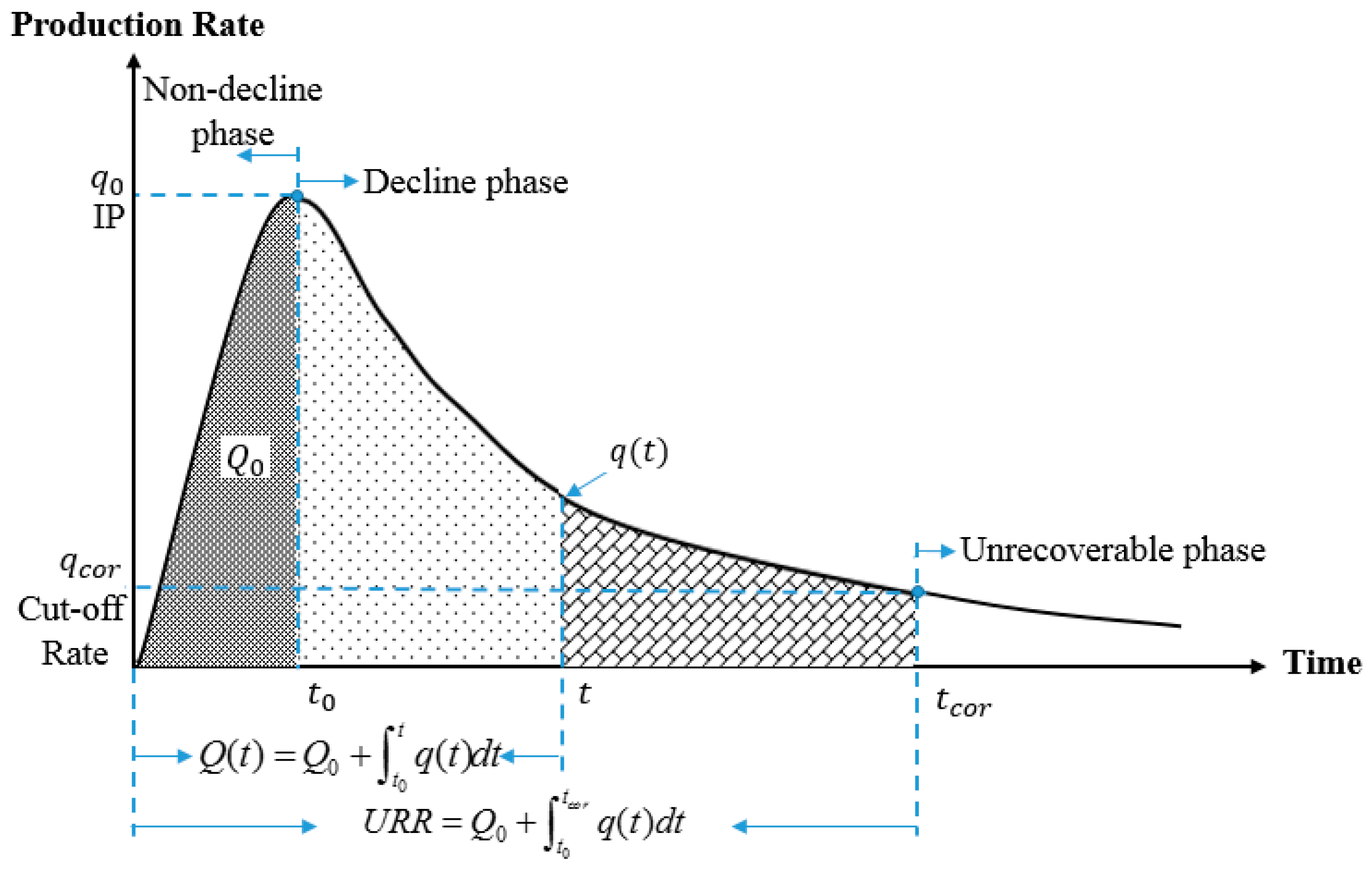
2.1. Decline Curve Models

Depletion occurs when any resource is extracted faster than it can be reproduced by nature [12]. Hydrocarbon resources are only reproduced on geological time scales than require millions of years, while manmade extraction takes years or decades at most. This makes hydrocarbon irreversibly unsustainable for all practical purposes, yet their exploitation is important for many aspects in modern society.
Decline curve analysis is a methodology focused on fitting observed production rates of a single well, or group of wells, by a mathematical function to predict future performance in the future by extrapolating the fitted decline curve function [13,14]. It has been around since 1940s and is used as a benchmark for simple well analysis. The original framework presented by Arps [15] has been proven to be easy to implement and useful for describing and predicting production in conventional oil and gas wells. The decline rate, denoted by λ, can be expressed using derivatives with production rate q and time t, as shown in Equation (1):
λ = d q / d t q = C q β
In the Equation, C is a constant and β is the decline exponent. Arps identifies three types of production rate decline behavior: Exponential (when β = 0, Equation (2)), Hyperbolic (when 0 < β < 1, Equation (3)), and Harmonic (when β = 1, Equation (4)):
q ( t ) = q 0 e λ ( t t 0 ) ,
q ( t ) = q 0 [ 1 + λ β ( t t 0 ) ] 1 / β ,
q ( t ) = q 0 [ 1 + λ ( t t 0 ) ] 1 ,
where q ( t ) is the production rate at time t, and q 0 is an initial production rate at time t 0 from which production begins to decline.
The traditional Arps relations were derived for stable reservoir conditions with boundary-dominated flows and should only be used for situations with 0 < β < 1 [16,17]. Analysts occasionally allow β > 1 to obtain better fits, but this extend Arps curves beyond their original region of validity. In transient flow situations, usually lasting for months or even years in shale wells, the validity of hyperbolic decline falters due to very low reservoir permeability and this results in β >1 [18]. This is why β > 1 is allowed in the fitting of hyperbolic curves in this study.
To circumvent the limitations of the Arps curves, some new curves have been proposed. Such as the Stretched Exponential (SE) decline model [19], the Power Law (PL) model [16], and Duong’s model [20].
Two different decline curve models, the traditional Arps Hyperbolic model and the Stretched Exponential model, are selected and pitted against each other in this study. The advantages of these decline curves lie in the strong empirical compliance and ease of use with low requirements on input data. Their key properties are described in Table 1. In Section 3.2.3, the accuracy between the two selected models are compared based on the Eagle Ford case.
In the table, Q ( t ) is the cumulative production, Q 0 is the initial cumulative production when the decline starts, and URR is the estimated ultimate recoverable resource. In the stretched exponential method, q i , D i , and n are undetermined parameters; τ is equivalent to ( n / D i ) 1 / n [20].

2.2. Goodness of Fit
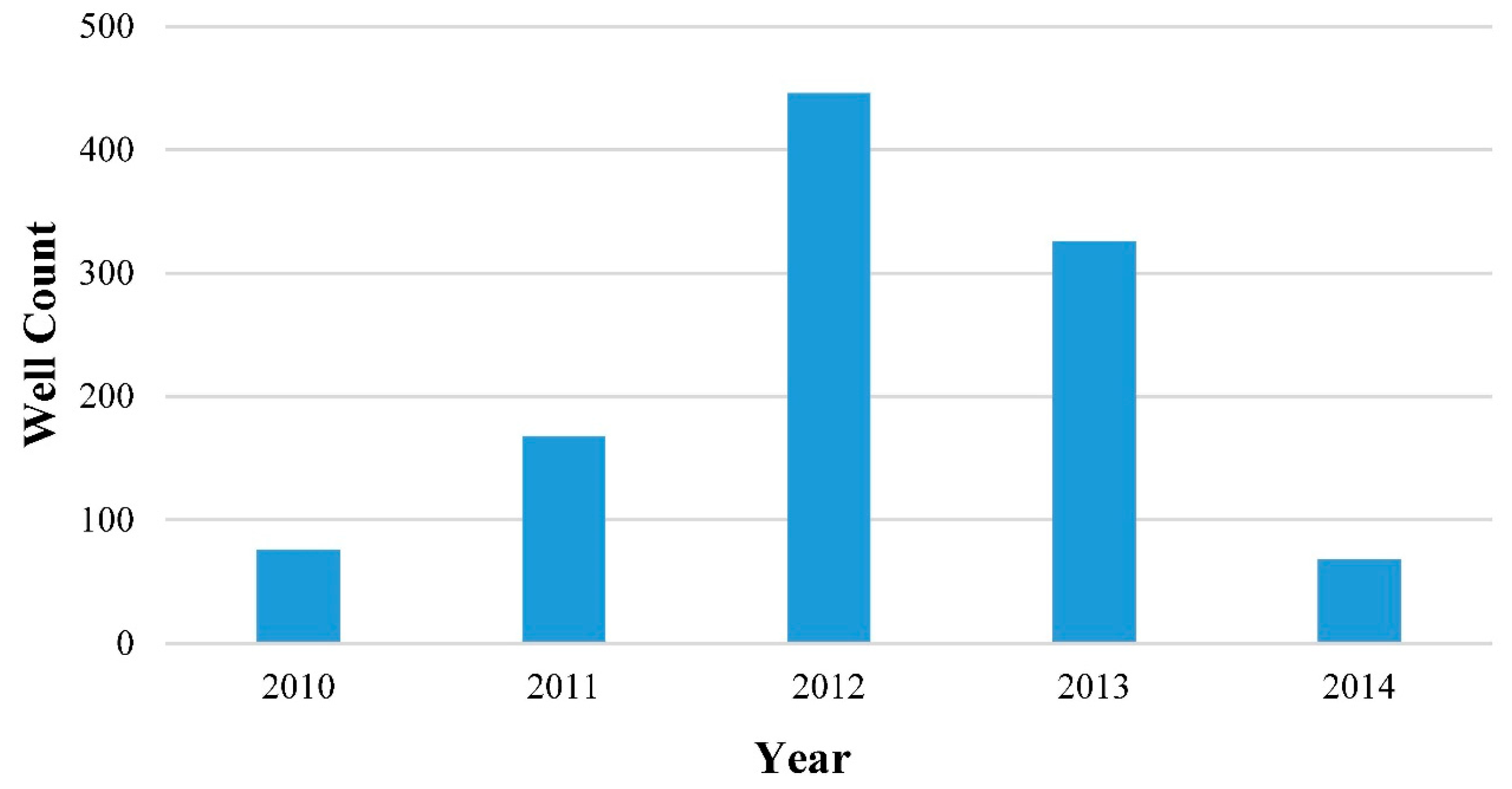
Matlab is used to fit the selected models to actual production data and assess how well the models represent the data. Both the coefficient of determination (R2) and the normalized root mean square error (N-RMSE) are used as measures for the goodness of fit [21,22]. R2 ranges from 0 to 1, and the goodness of fit will become better closer to 1. N-RMSE also ranges from 0 to 1, but here the goodness of fit will become weaker closer to 1. The boundaries that are introduced to exclude the poorest fits are R2 ≥ 0.8 and N-RMSE ≤ 0.2 at the same time.
Moreover, the number of observed data series should be long enough. According to the characteristics of shale industry and the data set, the period of two years (24 months) was set as the minimum number of production month to avoid over-fitting.

2.3. Data

The study is based on the monthly well-production data available from DrillingInfo [23], including 1084 shale gas wells that commenced production in January 2010 with data culminating in October 2014 in Eagle Ford. Only horizontal wells whose production is reported separately are included as the data samples used here. When production from several wells is reported together, the temporal distribution of the wells starting points also affects the overall production and this may obfuscate the characteristic production patterns of interest. Figure 2 shows the original number of wells in the data set per year.
Months with zero production should be removed before analysis, which is a measure to remove external events that affected production such as annual maintenance and scheduled downtime. Curve fitting of the aforementioned models is only done on production data from the decline phase. Figure 3 shows a stylized conceptual production curve with different production phases marked. The peak production point is also the initial production (IP) for the decline phase and one of the most influential factors for the total production. Pre-peak production is minor in comparison to post-peak production. On average, among the investigated wells in the study, the initial cumulative production ( Q 0 ) accounts for about 7% of their total well-production ( Q ( t ) ), and its percentage of URR would be even less, implying that the decline curve captures the vast majority of all production. The relation between Q 0 , Q ( t ) , and URR are also illustrated in Figure 3.

3. Results

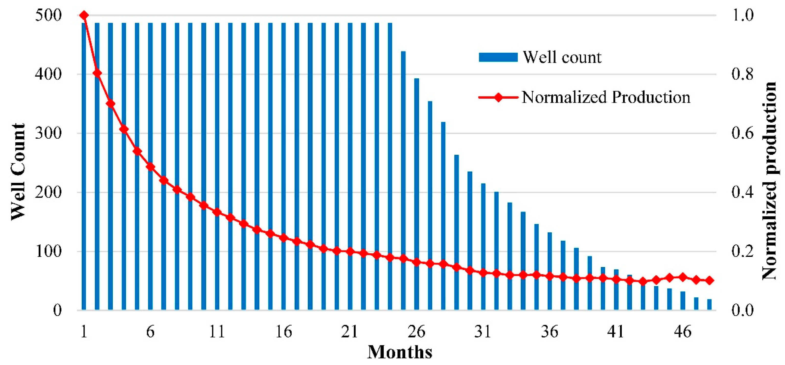
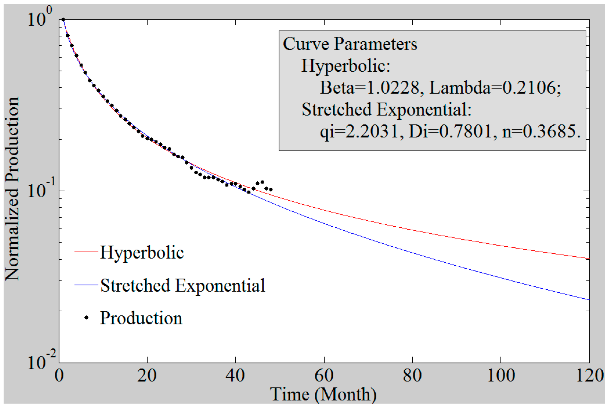
3.1. Aggregate Decline Curves

Wells with production data exceeding 24 months are normalized well by well in the sense that the peak production (marked as IP, initial production, in Figure 3) is set to 1 and all following monthly productions are displayed in relation. The aggregated normalized production of the first four years (48 months) and well count used for different months are shown in Figure 4. The tail of the production curve is less certain than the early months as the number of data points shrinks over time. However, it is clear that decline slows down with time. The annual decline over the first year of production is 68.54%, while it is only 43.08% over the second year. Over the first two years, production declines by 82.09% from the initial production level.
Hyperbolic and SE models are fitted to the aggregated normalized production from the Eagle Ford wells. Resulting fits are very similar and hard to distinguish on a regular plot, and for this reason a logarithmic scale is used in Figure 5. Both curves have excellent goodness of fit using R2 and N-RMSE. For the Hyperbolic model, the R2 value is 0.9987 and the N-RMSE value is 0.0073. In comparison, the Stretched Exponential model has an R2 value of 0.9985 and an N-RMSE value of 0.0080. The parameter values of the curves are also shown in the text box in Figure 5.

3.2. Individual Well Decline Curves

Wells with production data exceeding 24 months are also fitted one by one using both Hyperbolic and Stretched Exponential models. This provides an alternative insight into well behavior compared to aggregating production data prior to curve fitting.

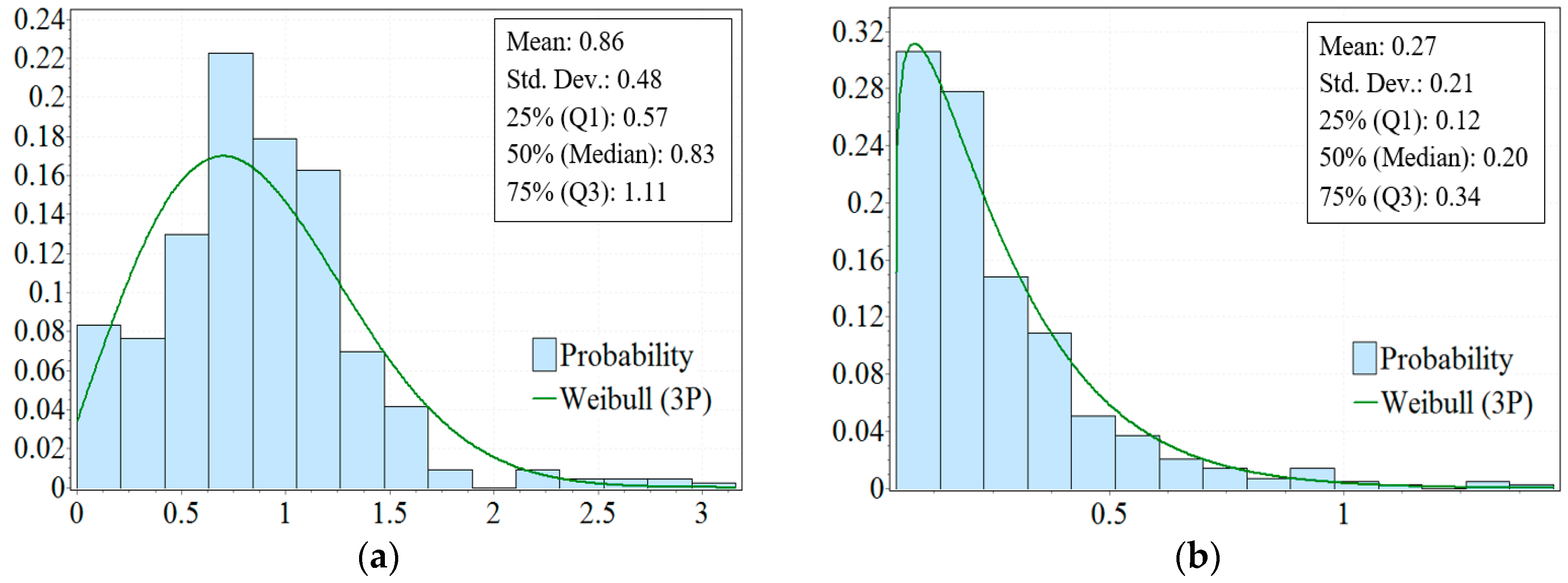
3.2.1. Hyperbolic Decline Curve

The distributions for the best fitted β and λ values of the Hyperbolic fits are displayed in Figure 6a,b respectively with their key descriptive statistics attached in the textboxes. The Weibull distribution (Three parameters: Weibull (3P) probability density function is f ( x ) = α β ( x γ β ) α 1 exp [ ( x γ β ) α ] , where α, β, and γ are fitted parameters.) is one of the best descriptions for the probability distributions according to Chi-Squared tests and this reflects the earlier results found for conventional oil by Höök [24].
The largest value is 3.16 for β and about 37% of the β values are larger than 1, and values between 0.4 and 1.6 make up about 80% of all occurrences (Figure 6).

3.2.2. Stretched Exponential Decline Curve

Some key descriptive statistics of the best fitted parameters for the Stretched Exponential decline curves are shown in Table 2.

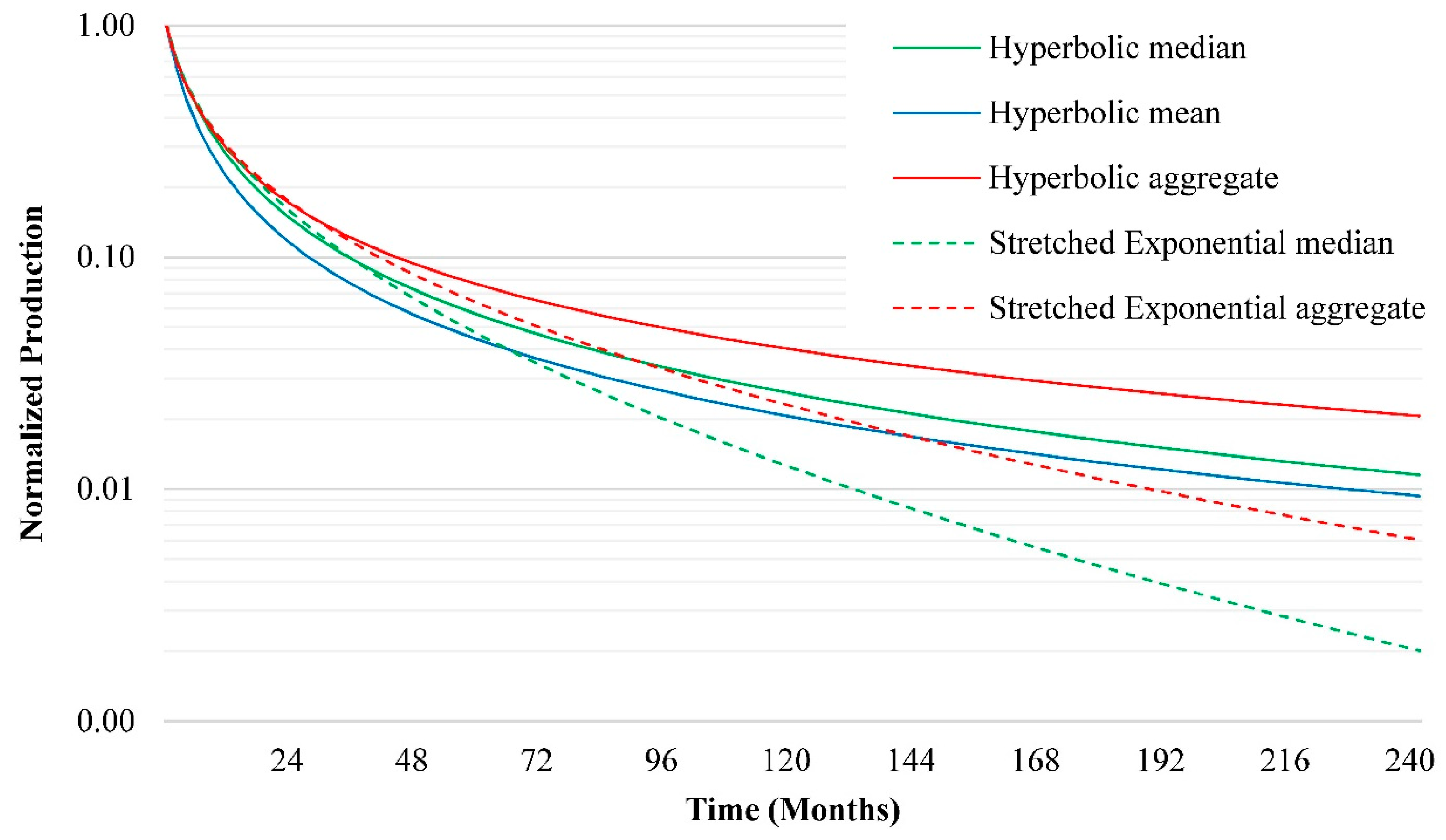
3.2.3. Summary of Decline Curves

The typical decline curves for shale gas production are derived from historical production profiles by using Hyperbolic and SE models. Both models fit aggregated well and individual shale gas well production data. Comparing goodness of fit indicates that Hyperbolic curves are slightly better fits than Stretched Exponential curves for about 65% of the wells according to R2 and for about 76% of all wells using N-RMSE. However, the result maybe only represents the Eagle Ford case. Longer data series and larger databases are needed to find out which model is better on a greater scale.
Figure 7 provides a summary of different derived characteristic decline curves investigated in this study, including median and mean versions of the two models. However, the parameters of the SE model are interconnected and by taking the mean, the connection will be lost. In Figure 7, the aggregate decline curves (see Figure 5) are also displayed. The aggregate curves (the red solid line and red dotted line) of two models are declining more gradually than their corresponding mean or median lines. The Stretched Exponential median curve (green dotted line) declines steepest in a medium to a long term perspective while the Hyperbolic median and mean curves (green solid line and blue solid line) decline fast initially after which they flatten out.

3.3. Initial Production and Decline Rate

The initial production (IP) at the onset of decline, i.e. peak production, and the decline rates in different time phases of the production curve are also analyzed for all wells with production data exceeding 24 months.

3.3.1. Initial Production

The distributions for the monthly IP for all wells that started production in 2010–2012 are displayed in Figure 8. About 77% of all wells reach a production peak ranging from 50,000 to 150,000 Mcf per month. As shown in the textbox in Figure 8, the mean IP of every well is 99.4 Mcf per month or about 3267 Mcf per day (Mcf/d).

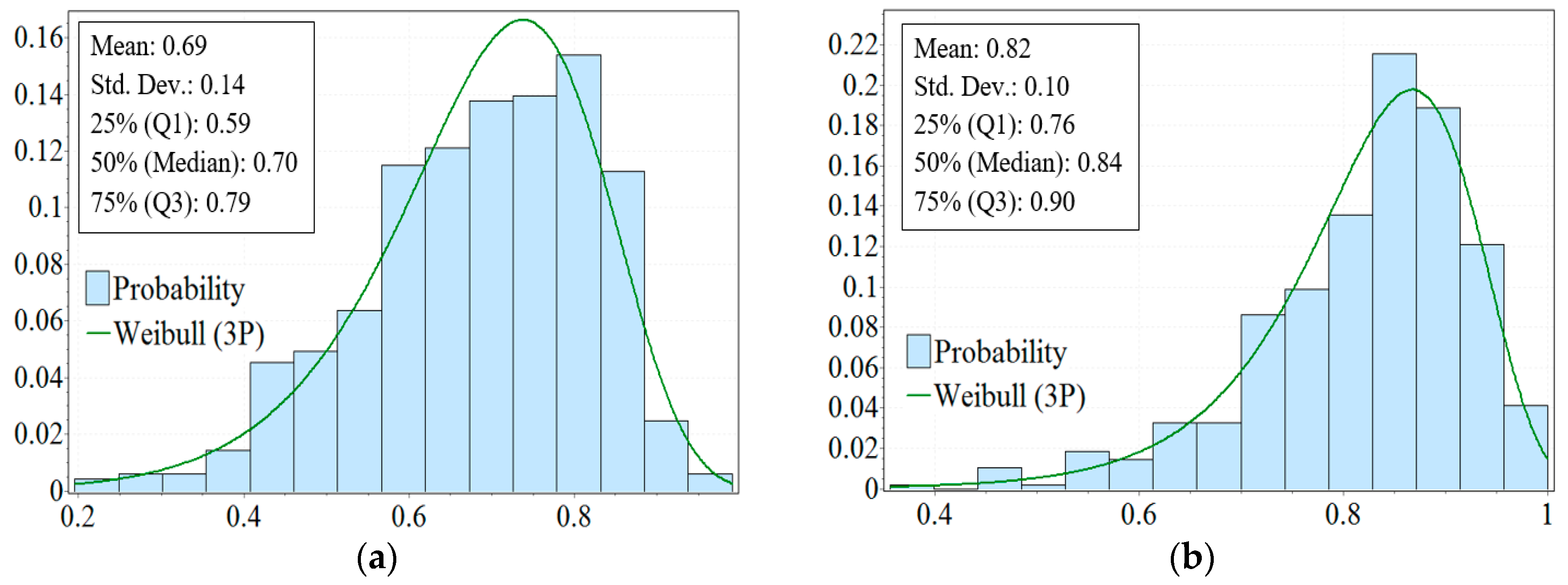
3.3.2. Decline Rates in Different Time Phases

The distributions for the first year (12 months after IP), decline rates, and the decline rates over the first two years (24 months after IP) of every studied wells are displayed in Figure 9a,b, respectively.
The average value of the first year decline rates for all wells started in 2010–2012 is 68.54% and the first two years decline rate is 82.09%; for the annual results, the first year and first two years average decline rates are shown in Table 3.

3.4. Estimated Cumulative Production

At some point, a shale gas well will experience a cut-off rate for continued production (due to technical and economic limits, q c o r in Figure 3), as production flows simply become too low to merit continued operation. Then the ultimate production can be described at the cumulative production over the well’s life time to final shutdown, and the estimated Q ( t ) at the time where the cut-off rate appear ( t c o r ) can used as an estimate for URR. Kaiser and Yu [25] found that typical wells in Texas are shut down and retired at an average annual production of 5 boe/d. However, the scope of this study does not allow deeper analysis of the economic aspects of shale gas production and projections on future profitability. Instead, assumed life spans are used as an alternative approach.
Applying characteristic decline curves from Figure 8, the mean value of the peak production of 3267 Mcf/d and supposed producing time length of 10-year, 15-year, 20-year, and 30-year are used to estimate expected cumulative production Q ( t ) . The average initial cumulative production before the peak is 72,078 Mcf, which is equivalent Q 0 in the Q ( t ) functions shown in Table 1. The results are displayed in Table 4.
Production levels would be very low about 10 years after the peak and could be below the economic limit due to characteristic high decline rates. Hence, assumptions of very long life spans (>20 years) for shale wells must be properly grounded. Using a 20-year well life span, shale gas wells were estimated to yield an URR of 1.41 to 2.03 Bcf based on the two decline curve models. Some estimated URR values for typical shale wells found in other studies are summarized in Table 5. There are significant differences among published estimates due to the short operation history of large-scale shale gas exploitation. For example, mean estimates for URR ranges from 1.0–5.0 Bcf/well in Table 5. Among the studies listed in Table 5, the EIA gives the highest estimate of URR, which is far different from later studies. The main reasons include: (1) the EIA did not estimate the URR and other average properties by itself instead of introducing results reported by some companies such as Petrohawk Energy, Talisman Energy, and Rosetta Resources; (2) the Eagle Ford shale was first discovered by Petrohawk in 2008, so the production history of drilling horizontal wells in the Eagle Ford shale was too short for good URR estimation in 2011. Similar problem also appeared in Baihly’s study in 2010. The result of this study is more accurate based on longer and relatively complete data compared with earlier studies. Also, the used goodness-of-fit measures also improve the results. In addition, this study indicates that the lower span of this interval is more reasonable, but more research is encouraged to illuminate this issue further.

4. Conclusions

This study found that, most of all, investigated shale gas wells in the Eagle Ford shale play have a characteristic production pattern characterized by quickly reaching a peak production followed by steep declines (~70% per annum) and low long-term production levels. As shown in the results section, the first annual year decline rate of production of a shale gas well is around 70% and over the first two years about 80% of the initial production level is lost due to decline, which is far higher than that of conventional natural gas. Furthermore, about 77% of wells reached the peak production from 50,000 to 150,000 Mcf per month or 1644 to 4932 Mcf per day. Raising outputs significantly from shale gas wells by enhancing recovery efficiency technology is also an efficient way to counteract this high decline rate.
Sustaining shale gas production in long-term energy strategies requires proper planning to handle the challenges imposed by the characteristic production patterns. A large number of “new wells” are annually needed to offset the production decline from the “old wells” to maintain regional production levels or increase production output. This is both a logistic challenge in maintaining a host of active drilling rigs, but also a social challenge to obtain acceptance for high drilling activity. Holistic analysis that includes economic balance based on the characteristic shale gas production pattern as well as logistics of the necessary drilling activities are essential to pinpointing the best options for developing a shale play.
According to the results of goodness-of-fit (R2 and N-RMSE), both the Hyperbolic model and the Stretched Exponential model fits well to aggregated well data and to individual wells. The Hyperbolic model is slightly better than the Stretched Exponential model based on the Eagle Ford case in this study, there are about 37% of the β-parameter values of Hyperbolic larger than 1. However, further research is needed to find out which model is better on a greater scale. On average, shale gas wells were estimated to yield an URR of 1.41 to 2.03 Bcf based on the two decline curve models when 20 years was set as well life span, which is in line with some other studies. As mentioned in the methodology Section 2.1, the traditional Arps model (Hyperbolic) was supposed to be used only for describing and predicting production in conventional oil and gas wells. While this study indicates that it is still effective for a shale gas well if the life span is set reasonably (20 years, for example). Deeper analysis of the economic aspects, such as the cut-off-rate for continued production and further research with more accuracy, are still needed to be able to estimate the future production and resources.
Available production data is still fairly limited for long-term trend analysis, since large scale shale gas operations have only been ongoing for barely a decade. The “American experience” is the only source of empirical data for shale gas production behavior and it serves as a suitable foundation for any attempt to describe or predict future shale gas developments. Production patterns of shale gas wells have general characters, even though the geological conditions for shale plays may vary. The findings of this study provide better understanding of characteristic production behavior and what to expect from shale gas production. The parameters of the models analyzed in the study can be adjusted to describe and predict shale gas production beyond the Eagle Ford shale, and beyond North America. Hence, the findings are relevant for analysts and policymakers to understand and provide access to energy resources required for future development.

Acknowledgments

The authors would like to thank DrillingInfo for providing access to their extensive database, without which this study would have been difficult to accomplish. The authors also would like to give many thanks to the National Social Science Foundation of China (No. 13&ZD159) for sponsoring this research. This study has been supported by the StandUp for Energy collaboration initiative.

Author Contributions

Mikael Höök and Baosheng Zhang conceived and designed the experiments; Keqiang Guo performed the experiments; Keqiang Guo and Mikael Höök analyzed the data; Kjell Aleklett contributed data; Keqiang Guo wrote the paper.

Conflicts of Interest

The authors declare no conflict of interest. The founding sponsors had no role in the design of the study; in the collection, analyses, or interpretation of data; in the writing of the manuscript, and in the decision to publish the results.

Abbreviations

The following abbreviations are used in this manuscript:
SEStretched Exponential
TcfTrillion cubic feet
BcfBillion cubic feet
McfMil cubic feet = Thousand cubic feet
URRUltimate recoverable resource

References

  1. Jackson, J.A. Glossary of Geology, 4th ed.; American Geosciences Institute: Alexandria, WV, USA, 2011. [Google Scholar]
  2. Technically Recoverable Shale Oil and Shale Gas Resources: An Assessment of 137 Shale Formations in 41 Countries Outside the United States. Available online: http://www.actu-environnement.com/media/pdf/news-23433-rapport-aie.pdf (accessed on 31 July 2015).
  3. Wang, Z.; Krupnick, A. A Retrospective Review of Shale Gas Development in the United States: What Led to the Boom? Available online: http://www.rff.org/files/sharepoint/WorkImages/Download/RFF-DP-13-12.pdf (accessed on 2 July 2015).
  4. BP Statistical Review of World Energy 2016. Available online: http://www.bp.com/statisticalreview (accessed on 20 June 2016).
  5. Erdogdu, E. Bypassing Russia: Nabucco project and its implications for the European gas security. Renew. Sustain. Energy Rev. 2010, 14, 2936–2945. [Google Scholar] [CrossRef] [Green Version]
  6. Lu, W.; Su, M.; Fath, B.D.; Zhang, M.; Hao, Y. A systematic method of evaluation of the Chinese natural gas supply security. Appl. Energy 2016, 165, 858–867. [Google Scholar] [CrossRef]
  7. U.S. Energy Information Administration (EIA). Annual Energy Outlook 2014 with Projections to 2040. Available online: http://www.eia.gov/forecasts/archive/aeo14/ (accessed on 7 May 2014).
  8. Toscano, A.; Bilotti, F.; Asdrubali, F.; Guattari, C.; Evangelisti, L.; Basilicata, C. Recent trends in the world gas market: Economical, geopolitical and environmental aspects. Sustainability 2016, 8, 154. [Google Scholar] [CrossRef]
  9. Annual Energy Outlook 2016 Early Release: Annotated Summary of Two Cases. Available online: http://www.eia.gov/forecasts/aeo/er/pdf/0383er(2016).pdf (accessed on 10 July 2015).
  10. Pi, G.; Dong, X.; Dong, C.; Guo, J.; Ma, Z. The status, obstacles and policy recommendations of shale gas development in China. Sustainability 2015, 7, 2353–2372. [Google Scholar] [CrossRef]
  11. Hu, D.; Xu, S. Opportunity, challenges and policy choices for China on the development of shale gas. Energy Policy 2013, 60, 21–26. [Google Scholar] [CrossRef]
  12. Höök, M.; Bardi, U.; Feng, L.; Pang, X. Development of oil formation theories and their importance for peak oil. Mar. Petrol. Geol. 2010, 27, 1995–2004. [Google Scholar] [CrossRef]
  13. Höök, M.; Davidsson, S.; Johansson, S.; Tang, X. Decline and depletion rates of oil production: A comprehensive investigation. Philos. Trans. R. Soc. Lond. Math. Phys. Eng. Sci. 2014, 372, 20120448. [Google Scholar] [CrossRef] [PubMed]
  14. Khanamiri, H. A non-iterative method of decline curve analysis. J. Pet. Sci. Eng. 2010, 73, 59–66. [Google Scholar] [CrossRef]
  15. Arps, J.J. Analysis of decline curves. Trans. AIME 1945, 160, 228–247. [Google Scholar] [CrossRef]
  16. Exponential vs. Hyperbolic Decline in Tight Gas Sands: Understanding the Origin and Implications for Reserve Estimates Using Arps’ Decline Curves. Available online: https://www.researchgate.net/profile/Thomas_Blasingame/publication/254528784_Exponential_vs_Hyperbolic_Decline_in_Tight_Gas_Sands_Understanding_the_Origin_and_Implications_for_Reserve_Estimates_Using_Arps'_Decline_Curves/links/569c06b808ae6169e56278a3.pdf (accessed on 1 July 2015).
  17. Ahmed, T. Reservoir Engineering Handbook, 3rd ed.; Gulf Professional Burlington: Burlington, MA, USA, 2006. [Google Scholar]
  18. Bailey. Decline rate in fractured gas wells. Oil Gas J. 1982, 80, 117–118. [Google Scholar]
  19. Valko, P.P. Assigning value to stimulation in the Barnett Shale: A simultaneous analysis of 7000 plus production histories and well completion records. In Proceedings of the SPE Hydraulic Fracturing Technology Conference, The Woodlands, TX, USA, 19–21 January 2009.
  20. Duong, A.N. Rate-Decline Analysis for Fracture-Dominated Shale Reservoirs. Available online: http://www.pe.tamu.edu/blasingame/data/z_zCourse_Archive/P648_15A/P648_15A_Lectures_(working_lectures)/20150420_P648_15A_Lec_19_SPE_137748_[pdf].pdf (accessed on 1 April 2015).
  21. Wang, J.; Feng, L.; Zhao, L.; Snowden, S.; Wang, X. A comparison of two typical multicyclic models used to forecast the world’s conventional oil production. Energy Policy 2011, 39, 7616–7621. [Google Scholar] [CrossRef]
  22. Patzek, T.W.; Croft, G.D. A global coal production forecast with multi-Hubbert cycle analysis. Energy 2010, 35, 3109–3122. [Google Scholar] [CrossRef]
  23. Drillinginfo. Available online: http://info.drillinginfo.com/ (accessed on 20 June 2015).
  24. Höök, M. Depletion rate analysis of fields and regions: A methodological foundation. Fuel 2014, 121, 95–108. [Google Scholar] [CrossRef]
  25. Kaiser, M.J.; Yu, Y. Economic limit of field production in Texas. Appl. Energy 2010, 87, 3235–3254. [Google Scholar] [CrossRef]
  26. Gong, X. Assessment of Eagle Ford Shale Oil and Gas Resources. Ph.D. Thesis, Texas A&M University, College Station, TX, USA, August 2013. [Google Scholar]
  27. Hughes, J.D. Drill, Baby, Drill: Can Unconventional Fuels Usher in a New Era of Energy Abundance? Post Carbon Institute: Santa Rosa, CA, USA, 2013. [Google Scholar]
  28. U.S. Geological Survey Oil and Gas Assessment Team. Variability of Distributions of Well-Scale Estimated Ultimate Recovery for Continuous (Unconventional) Oil and Gas Resources in the United States. Available online: http://pubs.usgs.gov/of/2012/1118/OF12-1118.pdf (accessed on 1 June 2012).
  29. Swindell, G.S. Eagle Ford Shale—An Early Look at Ultimate Recovery. In Proceedings of SPE Annual Technical Conference and Exhibition, San Antonio, TX, USA, 2012.
  30. U.S. Energy Information Administration (EIA). Review of Emerging Resources: U.S. Shale Gas and Shale Oil Plays. Available online: https://www.eia.gov/analysis/studies/usshalegas/pdf/usshaleplays.pdf (accessed on 8 July 2011).
  31. Baihly, J.D.; Altman, R.M.; Malpani, R.; Luo, F. Shale Gas Production Decline Trend Comparison over Time and Basins. In Proceedings of the SPE Annual Technical Conference and Exhibition, Florence, Italy, 20–22 September 2010.
Figure 1. US natural gas production by sources, 1990–2040; Source: EIA 2014 [7].
Sustainability 08 00973 g001
Figure 2. The original number of wells (1084 in total).
Sustainability 08 00973 g002
Figure 3. The conceptual production curve.
Sustainability 08 00973 g003
Figure 4. The aggregate decline curve.
Sustainability 08 00973 g004
Figure 5. The Hyperbolic and the Stretched Exponential decline curves fitted to average normalized production data on logarithmic scale. Only after 40 months do the two models start to diverge.
Sustainability 08 00973 g005
Figure 6. (a) Distributions of β values. β values are on the x-axis and the probability on the y-axis, the Weibull parameters are α = 2.13, β = 1.11, γ = −0.13; (b) Distributions of λ values. λ values are on the x-axis and the probability on the y-axis, the Weibull parameters are α = 1.15, β = 0.23, γ = 0.04.
Sustainability 08 00973 g006
Figure 7. Summary of different derived typical decline curves (on logarithmic scale).
Sustainability 08 00973 g007
Figure 8. Distributions for the monthly IP. Production is on the x-axis and the probability is on the y-axis; production unit is Mcf per month, the Weibull parameters are α = 2.63, β = 1.17 × 10⁵, γ = −5.29 × 10⁴.
Sustainability 08 00973 g008
Figure 9. (a) Distributions for the first year decline rates. Rates are on the x-axis and the probability is on the y-axis, the Weibull parameters are α = 14.27, β = 1.68, γ = −0.93; (b) Distribution for the first two years decline rate. Rates are on the x-axis and the probability is on the y-axis, the Weibull parameters are α = 8.16 × 10⁷, β = 6.52 × 10⁶, γ = −6.52 × 10⁶.
Sustainability 08 00973 g009
Table 1. Key properties of the Hyperbolic model and the SE model.
PropertiesHyperbolicSE
q ( t ) q 0 [ 1 + λ β ( t t 0 ) ] 1 / β q i   exp ( D i t n )
Q ( t ) Q 0 + q 0 λ ( 1 β ) { 1 [ 1 + λ β ( t t 0 ) 1 1 β ] } Q 0 + q i τ n { Γ [ 1 n ] Γ [ 1 n , ( t τ ) n ] }
URR Q 0 + [ q 0 / λ ( 1 β ) ] Q 0 + q i τ n Γ [ 1 n ]
Table 2. Descriptive statistics of the SE curves.
q i D i n
Mean138.951.390.49
Std. Deviation589.071.950.30
Min0.86<0.010.06
25% (Q1)1.340.270.28
50% (Median)1.840.580.45
75% (Q3)4.261.450.63
Max4608.888.462.78
Table 3. Average value of the first year and the first two years decline rates for new wells annually.
2010201120122010–2012
First year70.58%70.40%66.76%68.54%
First two years83.72%83.74%80.57%82.09%
Table 4. The average expected cumulative production per well.
10-Year15-Year20-Year30-Year
HyperbolicMedianq(t)85533823
Q(t)1.491.611.691.80
Meanq(t)68433119
Q(t)1.251.351.411.50
Aggregateq(t)132906846
Q(t)1.401.892.032.24
SEMedianq(t)411572
Q(t)1.441.491.511.52
Aggregateq(t)7636208
Q(t)1.581.681.731.78
Note: Unit for q(t) is Mcf/d and for Q ( t ) is Bcf (billion cubic feet).
Table 5. Summary of average estimated URR per well in Eagle Ford from other studies.
ReferenceMean URR (Bcf)Publish Time
Gong [26]1.45–3.782013
Hughes [27]2.362013
USGS [28]1.1042012
Swindell [29]1.0442012
EIA [30]5.02011
Baihly [31]3.7932010
This study
(20 years as well life span)
1.41–2.03

