Identifying Potential Area and Financial Prospects of Rooftop Solar Photovoltaics (PV)

Abstract

In an urban area, the roof is the only available surface that can be utilized for installing solar photovoltaics (PV), and the active surface area depends on the type of roof. Shadows on a solar panel can be caused by nearby tall buildings, construction materials such as water tanks, or the roof configuration itself. The azimuth angle of the sun varies, based on the season and the time of day. Therefore, the simulation of shadow for one or two days or using the rule of thumb may not be sufficient to evaluate shadow effects on solar panels throughout the year. In this paper, a methodology for estimating the solar potential of solar PV on rooftops is presented, which is particularly applicable to urban areas. The objective of this method is to assess how roof type and shadow play a role in potentiality and financial benefit. The method starts with roof type extraction from high-resolution satellite imagery, using Object Base Image Analysis (OBIA), the generation of a 3D structure from height data and roof type, the simulation of shadow throughout the year, and the identification of potential and financial prospects. Based on the results obtained, the system seems to be adequate for calculating the financial benefits of solar PV to a very fine scale. The payback period varied from 7–13 years depending on the roof type, direction, and shadow impact. Based on the potentiality, a homeowner can make a profit of up to 200%. This method could help homeowners to identify potential roof area and economic interest.

1. Introduction

A major concern regarding fossil fuel is that it creates environmental effects along with contributing to global warming [1]. In contrast to fossil fuels, renewable energy can be utilized as a remedy for solving the global warming problem. The development of renewable energy technology will promote sustainable development and reduce environmental impacts. Solar energy is an excellent energy source and uses the available power of the sun. The amount of sunlight that reaches a given area on the Earth’s surface varies according to the season, local landscape, time of day, geographic location, and local weather [2]. Thailand is geographically appropriate for utilizing solar energy, and this is less so for other renewable energy sources, such as hydroelectric power or wind [3]. Based on this prospect, Thailand has introduced the Alternate Energy Development Plan covering 2012–2021. The target for solar energy generation in 2021 is fixed to 2000 MW. One of the major initiatives in this regard is to support the installation of small systems at community and household levels, including rooftop solar photovoltaics (PV) to generate 1000 MW in 10 years. The National Energy Policy Council has shifted the motivational policy to a European style feed-in tariff (FiT) to decrease windfall profit and limit the price effect to the end consumers. FiT is 6.96 Thai baht (THB) per kilowatt hour for small-to-medium-sized systems and households producing not more than 10 kW, while for those that generate 11 to 250 kW, the rate is 6.55 baht, and 6.16 baht for those making 251 kW or more. The government will provide FiT for 25 years [4] based on the life span of the solar panel.

In an urban area, the roof is the only available surface that can be used for installing solar PV, and the active area depends on the type of roof. Roof area identification takes substantial effort in finding out the potential of solar PV on buildings [5]. Building footprints and floor data are available from different government agencies in Thailand, but the type of roof, along with the direction, is absent in most databases. Researchers have utilized high-resolution satellite images and Object Base Image Analysis (OBIA) to extract and classify features [6,7,8,9,10]. Separate techniques have been developed to generate a three-dimensional (3D) model of structures. Huang et al. [11] presented a semi-automated approach to high-quality 3D object reconstruction from single high-resolution satellite images using a mono-plotting technique. The method requires a highly accurate satellite sensor model. Vosselman and Dijkman [12] implemented a 3D version of the well-known Hough transform. López-Fernández et al. [13] deployed the multi-sensor aerial platform to identify and classify roof surfaces for setting solar panels. This system applies to the less dense areas, and they did not simulate shadows from surrounding areas. Very high computational power is required to process the data.

The Geographical Information System (GIS) has been used to identify potential areas for solar PV. The model developed by Fu and Rich [14] implemented an ArcMap GIS Extension, known as the Solar Radiation Toolset, which is suitable for a fine scale. Based on a digital terrain model, it generates a view shed. Another model developed by Wilson and Gallant [15], the SRAD model, was designed to model topographic and mesoscale processes of the landscape. Suri and Hofierka [16] developed a solar radiation model, called r.sun, within the GRASS GIS environment. Different researchers [17,18,19,20,21,22,23] have presented other computational solar radiation models. The analysis of shadows on building height, location, and roof type is missing from all of these models. Shadows on a solar panel can be generated by nearby tall buildings, construction materials such as water tanks, or the roof configuration itself. The azimuth angle of the sun varies based on the season and time of day, so the shadow effect is not static. Izquierdo et al. [24] studied the influence of hourly shadows on monthly values via geometrical calculations with digital terrain models; the results show that the shadowing coefficient varies from 0.33 to 0.52, depending on the municipality type (as a function of population and building densities) in Spain. Jo et al. [25] utilized Google SketchUp for shadow analysis, a 3D computer modeling program able to cast shadows based on the longitude and latitude of the site. The result of the study (which included 932 buildings) was that about 30% of the total rooftop area of unshaded, predominately flat, roofs were suitable for PV applications. Ordonez et al. [26] calculated shadows cast by different construction elements (e.g., chimneys, elevator shafts, etc.) using the AutoCAD software program. The study concluded that the useful rooftop surface area, where a PV array could be mounted, was 82% of the total roof area. As shadow analysis is very challenging and depends on local factors, such as surrounding buildings, vegetation, etc., many researchers have used a rule of thumb for identifying unshaded rooftops. LiDAR has become popular in recent years due to its resolution and effectiveness. Researchers used LiDAR technology for detecting city buildings [27], trees, and roof structures [28], identifying the potential solar radiation of built areas [29] and even for solar mapping [30]. However, this technology is expensive and requires extensive infrastructure and expertise [31]. Shadowing effects due to tree leafs lead to non-negligible power losses of solar PV modules [32] and reduce efficiency [33]. This analysis is missing in the recently introduced Google Sunroof project (https://www.google.com/get/sunroof#p=0). This tool is used to calculate the best solar plan for homeowners. It utilizes expensive aerial photographs, the Google database, and other computing resources to identify areas that are available for setting solar panels. The major drawback of this system is that it is only applicable to the United States (due to aerial photograph availability) and, in many cases, overestimates suitable areas (Figure 1).

The simulation of shadow for one or two days or using the rule of thumb may not be sufficient to evaluate the shadow effect on solar panels throughout the year. The area available on different faces of the roof also plays a great role in potential area calculations and financial prospects. The homeowner will be more interested if the potential area is accurately assessed and the economic opportunity is very clear, as they have to spend a significant amount of money to install solar PV on the roof. Most of the previous research has focused on the identification of roof area available for solar PV based on the extraction of the roof from a satellite image. None of them has attempted to classify roof type from a single satellite image. The shadow factor is considered by assumption or by testing one or two buildings for a couple of days and then applying a rule of thumb to the whole area. However, the shadow can be cast by the nearby tall buildings, construction material, or most importantly by the roof configuration itself. The facing of the roof is estimated based on a literature survey. The major drawback of those systems is that the calculation can provide only an idea of the potential area. Those are also location-specific, as data used for one country may vary in another country.

In this paper, a remote sensing and GIS-based methodology that accounts for individual building characteristics are presented for estimating solar potential on multiple building rooftops. The scope of this article is as follows: (i) classifying roof types from very high-resolution satellite images; (ii) simulating shadow effects throughout the year; and (iii) identifying potential areas and the financial prospects of rooftop solar PV systems. This study concentrates only on the shadow effect from surrounding buildings and the building itself. It does not analyze other shading factors such as trees, pylons, construction materials such as chimneys, and elevator shafts.

2. Materials and Methods

2.1. Study Site

Bangkok is the capital of, and the most populous city in, Thailand. Bangkok is located on a flat plane, and sunlight hours vary from 5 to 9 h [34]. The city inhabits 1568.7 km² in the Chao Phraya River delta in Central Thailand. A large number of structures have been developed to accommodate the large number of people. In Bangkok, structures are of different heights and sizes with different roof types. In this research, the study area (Figure 2) was selected from the Chatuchak sub-district because of its diversity in roof type, height variation, orientation, and density. As indicated in Figure 2, buildings are very close to each other and trees are very low in height if available.

2.2. Dataset

Panchromatic and multispectral WorldView2 (GISTDA, Bangkok, Thailand) images were purchased from the Geo-Informatics and Space Technology Development Agency (GISTDA), Thailand. A number of floor data were collected from a field survey by visual inspection to develop 3D structures. Hourly solar radiation data were collected from the Thai Meteorological Department. These data were used for the calculating amount of solar radiation in the study area. Data regarding the installation cost of solar PV systems of various sizes were collected from two different local companies.

Table 1. Dataset used in the study with technical details.

Data Type	Source and Specification
WorldView2	Geo-Informatics and Space Technology Development Agency (GISTDA), Thailand Resolution: Panchromatic—0.46 m; Multispectral—1.85 m; Acquisition date: 8 January 2013
Solar Insolation for the year 2013	Thai Meteorological Department
Solar PV components and installation cost	Two local companies providing and installing solar PV
Number of floors	Field survey (visual inspection)
FiT Data	Department of Alternative Energy Development and Efficiency (DEDE)

contains the dataset used in this study with technical details.

2.3. Data Preparation

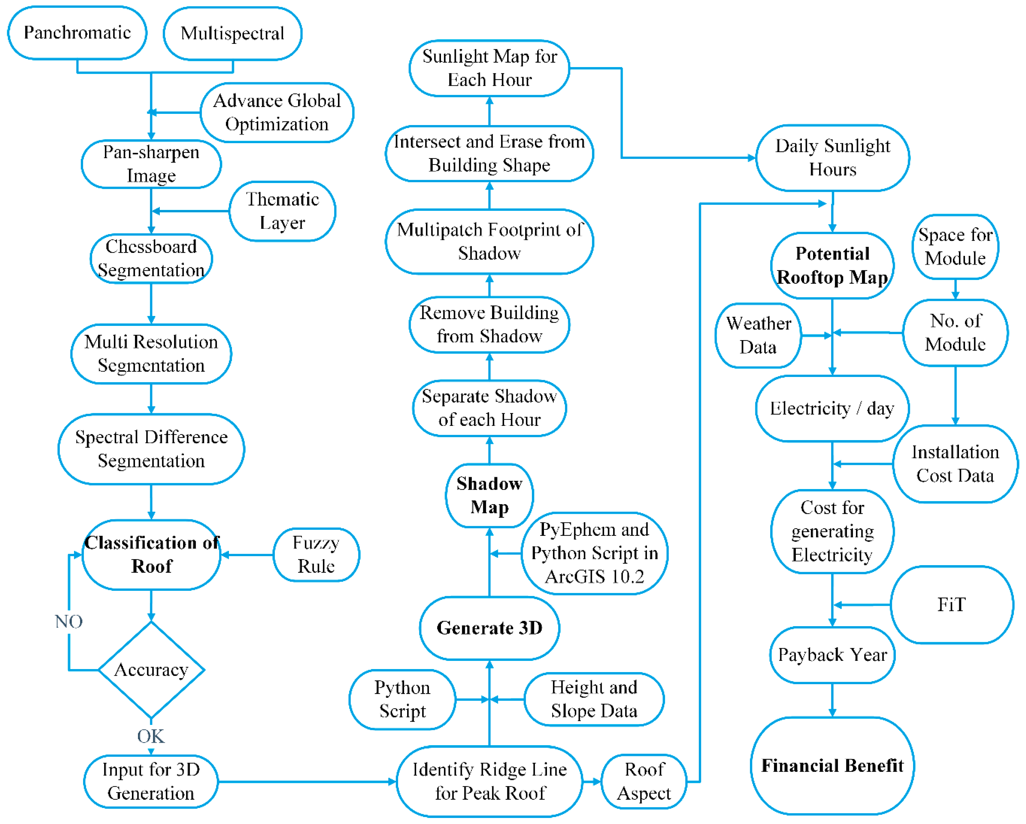
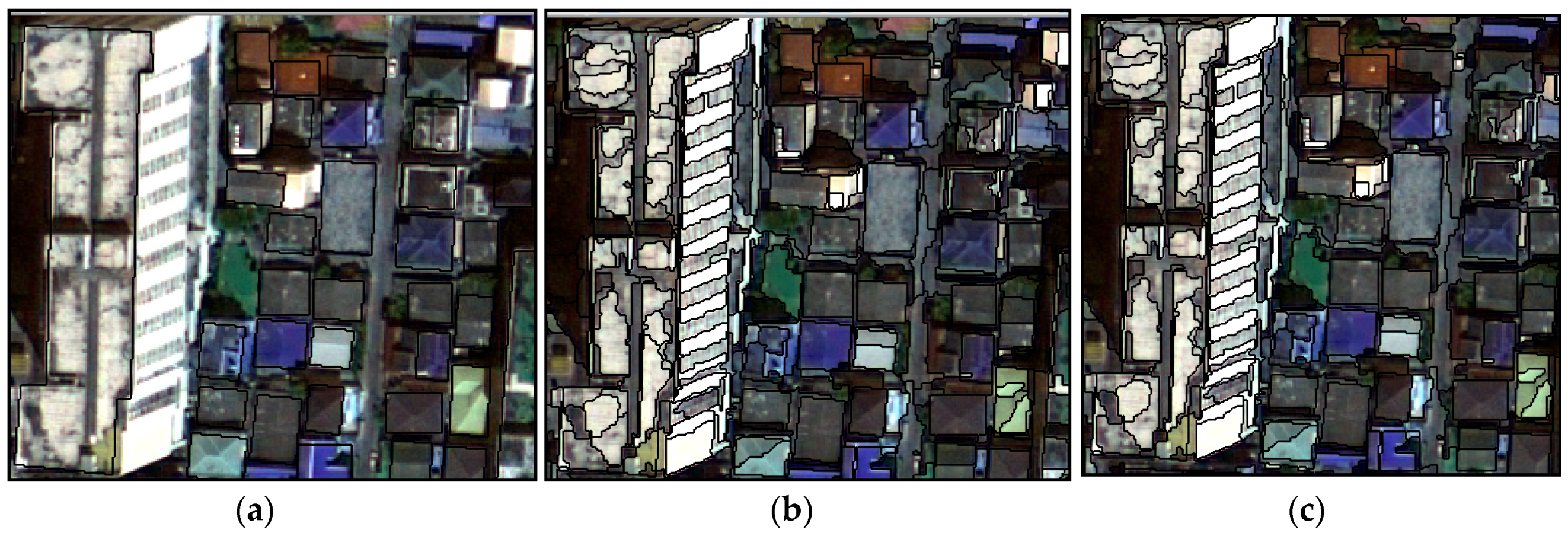
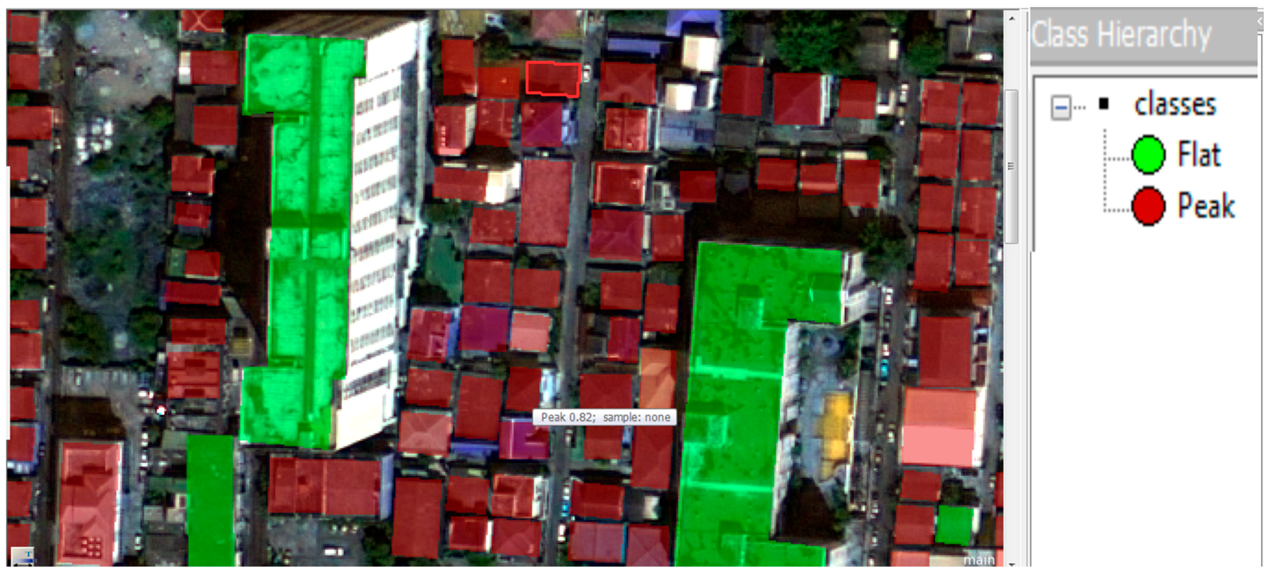
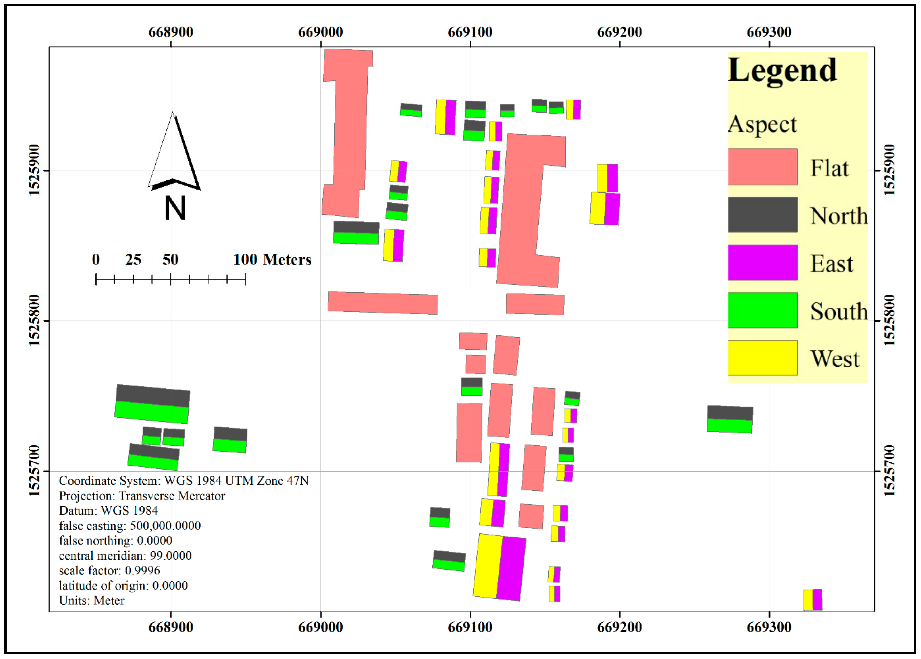
Data from WorldView2 with its 0.46 m panchromatic channel and three 1.85 m multispectral channels were well suited for image sharpening. The combination of multispectral and panchromatic bands was performed using HighView [35], a GeoSage commercial software, to make the best use of the high resolution of the panchromatic band. It applies an advanced global optimization algorithm for image sharpening. While the fused multispectral (MS) bands still retain the mean values of the original MS bands, their standard deviations naturally became larger due to the increased amount of detail and the heterogeneity of the image features in the fused MS bands. The obtained pan-sharpened color image had the same spatial resolution of the panchromatic image, with minimum spectral distortion [36,37].

2.4. Analysis

Firstly, the image segmentation and fuzzy rule implementation were performed to classify roof types as either peaked or flat. After the classification of roof types of each building, a 3D map of the structure was generated based on roof type, then the hourly shadow map was created for the whole year. Finally, the potential of each roof was calculated, and the financial prospect for each homeowner was identified. The overall methodology of this research is provided in Figure 3.

After pan-sharpening, image segmentation was performed as illustrated in Figure 4. Trimble’s proprietary software eCognition was used for this very purpose. Different levels of segmentation, i.e., chessboard segmentation (CS) for splitting the image into a square object [38] and multiresolution segmentation (MRS) for grouping similar objects (starting from each pixel), was carried out until a threshold representing the above object variance was reached [39]. CS is a top-down segmentation approach that cuts the scene or the devoted image objects into smaller objects [38]. Building blocks were digitized from the satellite image. Defining roofs (inserted building block as a thematic layer) by this method drastically reduced the number of units to be handled for the segmentation. The next step after mapping out roofs was to perform a multi-scale image analysis method. All parameters of MRS were assigned by trial and error [40,41], and one optimum set of parameters was chosen for the study area based on the visual inspection. Finally, spectral difference segmentation (SDS) was used for merging nearby objects based on the spectral mean.

Fuzzy membership thresholds (

Table 2. Fuzzy membership rule for classifying objects as peaked or flat.

Rule No.	Rule Description
1	For each spectral difference image object:
	IF compactness membership is high
	AND rectangular fit membership is high
	THEN P1 membership is high
	ELSE F1 membership is high
2	IF length/width ratio membership is high
	AND number of segments membership is high
	OR roundness membership is high
	THEN P2 membership is high
	ELSE F2 membership is high
3	IF P2 membership is high
	THEN Object label = Peaked
	ELSE Object label = Flat

) were implemented for the object features to describe and classify different classes. Compactness within the polygon, asymmetry, roundness, rectangular fit, length-width ratio, and the number of segments within the skeleton (in each roof) were used to classify roofs as either peaked or flat. The value for the membership function was fixed on a trial-and-error basis. To identify peaked roofs, initially rates were set as 1–1.5, 0–8, and 0–1 for compactness, number of segments, and roundness, respectively. After that, values ≥0.9 and 1–2 were fixed for the rectangular fit and the length–width ratio, respectively.

Height data was collected from a house-to-house survey. The number of floors was multiplied by 3.5 [42] to get the height of the structure in meters in the case of a flat-roofed house. In Thailand, most houses with a peaked roof have a slope of 45° [43]. This study used the 45° slope in addition to flat height to calculate the height of the ridge line in the case of a peaked roof. The width portion of the ceiling was identified to get the orientation of the ridgeline. Structures with rectangular shapes had a shorter width than length. The height of the roof edge was calculated from the number of floors and the ridge line from edge and slope. A triangulated irregular network (TIN) was generated to identify an aspect of each roof. A 3D image of the structure was produced in ArcScene 10.2 (Environmental Systems Research Institute (ESRI), Redlands, CA, USA). The Extrude Between tool in ArcScene 10.2 was used to create the 3D image. To generate a shadow map, the Sun Shadow Volume tool in the 3D Analyst extension, which used PyEphem and Python Script, was implemented under the ArcGIS 10.2 platform. A shadow volume map for each month was saved in one Personal Geodatabase file. The Sun Shadow Volume tool generated a shadow for each day in one feature class. A model was produced in ArcGIS Model Builder to isolate every hour in the shadow map. For each day, the model first selects one hour and saves that as one feature class. This process was done for all of the days in a month and then all of the months in the year 2013. Each hourly shadow map illustrated whether the roof of the building was shaded or not by the surrounding buildings or by itself at that particular moment.

While generating shadow maps in ArcGIS 10.2, buildings were also included in the shadow. The purpose of generating shadow maps was to identify the shaded part of the roof at that particular hour. Another model was produced in the Model Builder of ArcGIS 10.2 to remove the building from the shadow. The Difference 3D tool of the 3D Analyst was used, where 3D images of the buildings were added as a subtracting feature. The model iterates the same thing for the whole month and consequently for the year. The model has been used in ArcGIS 10.2 Model Builder to extract which part of the roof was getting sunlight in a given hour. The footprint of hourly shadow was generated and was intersected by the building shape to identify the shaded part. After that, from the shaded region, the building form was erased to extract the sunlight area. Lastly, the sunlight area was converted to raster for further analysis.

The hours of sunlight map generated in the previous section was multiplied by the efficiency of the particular face. The effectiveness of solar panels fixed facing east and west reduces to 85%, and that facing north reduces to 50% [44,45]. According to the North American Board of Certified Energy Practitioners (NABCEP) [44], a solar panel should be unshaded for at least six hours to produce maximum output. If the unshaded hours are eight or more, the solar panel can generate a significant amount of electricity throughout the year. While preparing the potential area map, this information was considered a criterion, along with the efficiency of the facing direction of the roof. Sunlight hours were multiplied by the effectiveness of the face to generate the potential area map. The study assumed that the homeowner would use polycrystalline PV modules with 295 watt-peak, which consist of 72 cells and would be set up in the landscape. The standard dimension of each module is 1956 × 992 × 50 mm. The shadow generated by the tool also creates a vertical angle for each hour of obscurity. By analyzing the data, it was observed that the lowest angle was 15.80°. It was assumed that houses with a flat roof will use a tilt angle of 10° while setting solar panels [46]. The spacing between rows of solar panels was calculated based on the tilt angle. For a peaked roof, 10 cm was kept at the edge of the module for air ventilation [44]. Therefore, the dimension of each module for a peaked roof was 2000 × 1100 × 150 mm and, for a flat roof, 2000 × 1600 × 50 mm. As illustrated in Equation (1), the potential area was divided by the dimension of the module to get the number of the modules that could be fixed.

$${\mathrm{NM}}_i={\mathrm{PA}}_i/\mathrm{MS},$$

(1)

where NM_i = number of modules that can be fixed on i-th roof; PA_i = potential area on i-th roof; MS = module size.

This study assumed that the installation cost of solar PV is the same for flat and peaked roof houses. Each 295 watt-peak module cost was 20,000 THB, including the required module and accessories. Total installation cost was calculated by multiplying the number of modules by the per module price (as provided in Equation (2)). Based on the weather data, it was observed that 75% hours in a day and 80% days in a year will get sunlight [34]. This information was incorporated into calculating electricity production by the module. From the number of modules, the module rating, shadow-free hours, and weather data, the amount of electricity that can be produced yearly is shown in Equation (3). The sum of money that can be earned each day was calculated by multiplying the generated kW in a day with the FiT amount for that range. By summing up all the days generating electricity, a yearly income was calculated. As illustrated in Equation (4), the payback period was calculated by dividing the installation cost by earnings in each year. If any fraction was found, it was rounded to the next number. FiT is available for 25 years; subtracting the payback period from this figure and multiplying it by the earnings per year showed the benefit of installing solar panels (Equation (5)).

$${\mathrm{INC}}_i={\mathrm{NM}}_i\times \mathrm{UCM},$$

(2)

where INC_i = installation cost for i-th roof; NM_i = number of module in i-th roof; UCM = unit cost of each module.

$${\mathrm{EPY}}_i={\displaystyle {{\displaystyle \sum }}_{j=1}^{j=365}}\left({\displaystyle {{\displaystyle \sum }}_{i=1}^{i=8}}{\mathrm{NM}}_i\times \mathrm{WP}\times {\mathrm{SFH}}_i\times \mathrm{CFH}\times \mathrm{RFD}\times \mathrm{FiT}\right),$$

(3)

where EPY_i = earning per year by i-th roof; NM_i = number of module in i-th roof; WP = watt-peak of the module; SFH_i = shadow free hours in each day of i-th roof; CFH = cloud free hours; RFD = rain free days; FiT = feed in tariff.

$${\mathrm{PBY}}_i={\mathrm{INC}}_i/{\mathrm{EPY}}_i,$$

(4)

where PBY_i = payback period of i-th roof; INC_i = installation cost for i-th roof; EPY_i = earning per year by i-th roof.

$${\mathrm{FIB}}_i=(\mathrm{FiT}\mathrm{year}-{\mathrm{PBY}}_i)\times {\mathrm{EPY}}_i,$$

(5)

where FIB_i = financial benefit from i-th roof; FiT year = feed in tariff year; PBY_i = payback period of i-th roof; EPY_i = earning per year by i-th roof.

3. Results and Discussion

Researchers have utilized remote sensing image to detect buildings [47] from shadow [48] and generated wire-frame building models [49,50], but have never tried to classify roofs. By applying OBIA in eCognition, the roof was classified as flat or peaked from a single remote sensing image, as presented in Figure 5. For the accuracy assessment purpose, a total of 91 structures were classified based on ground truth; among them, 61 were peak-roofed houses, and 30 were flat-roofed houses. The applied methodology can generate 98% of producer accuracy for peak-roofed house, but accuracy was low for flat-roofed house. Overall accuracy was 74%, which was satisfactory but not good enough. The reason for this result was that the roof type did not depend on spectral or even solely on spatial properties of the image object. The compactness of the peaked roofs was higher than a flat roof, but this was not true for old peak-roofed houses. The length–width ratio of flat-roofed houses was greater than that of peak-roofed houses, although some peak-roofed houses had the same characteristics. Due to compactness, the number of segments was higher in the case of flat-roofed houses and old peak-roofed houses. This classification was important for generating 3D structures, as the height of a roof varied based on the roof type. Peaked-roof houses had a maximum height at the ridge line.

It was observed that the ridge line was usually perpendicular to the width of the ceiling. The ridge line also indicates the azimuth of the roof, so the identification of the ridge line was an important part of generating 3D images. Apart from that, the orientation of the roof, especially for peaked roofs, was vital, as some parts of the canopy may be shaded even though other parts may receive sunlight at the same time. The study identified the ridge line along with the orientation of the housetop with absolute north (azimuth of the roof). After identification, accuracy was checked (RMSE 2.27°) by comparing the auto generated with the digitized sample. From the azimuth and the ridge line, the aspect of the roof was identified, as shown in Figure 6.

TIN was generated based on the height of each wall and ridge line. The Extrude Between tool in ArcGIS 10.2 was used to produce a 3D image (Figure 7) from the building footprint. From the figure, it is obvious that there were many low height structures near and in between two tall structures. The simulation of shadow for each individual structure was deemed necessary.

Whether the roof will be shaded (as seen in Figure 8) by the surrounding buildings or not depends on the building’s location with respect to tall buildings, and its height compared with the relevant tall building, as presented in Figure 9. A relationship has been developed with distance to identify whether the surrounding buildings will be shaded or not. The Sun rotates within an azimuth angle of between 23° and 317°, at the minimum in the month of June and maximum in the month of December. Based on this azimuth angle, the azimuth angle for the shadows was also calculated. If the low building is located within a 110°–250° azimuth of the taller building, then the low building will not be shaded for even in a single hour throughout the year.

Due to the angle created by the shadow at different times and months, the east and west-facing roofs received seven to eight hours of sunlight in a day until shaded by surrounding buildings (Figure 10). The south-facing roof received a full day of sunlight and the north-facing roof received fewer hours. Flat roofs had around nine hours of sunshine. However, the scenario completely changes when there are tall structures nearby. Section 1 in Figure 10 displays that, due to the adjacent tall structures, some parts of the structures were getting three hours of sunlight, and some five hours. The hours of receiving sunlight, even with nearby tall structures, depends on the height of the tall structure compared with the investigated building, the distance between them, and the location toward the actual azimuth.

It is worth mentioning that south-facing flat roofs had the most potential in most cases if not shaded by nearby tall buildings. East- and west-facing roofs also had potential, but a north-facing roof did not have potential. The result is similar to previous studies, such as those conducted by Jo et al. [25] and Ordonez et al. [26]. The electricity that can be generated in each year was calculated from the watt-peak rating of the module, sunlight hours per day, and the number of rain-free days in a year. The installation cost was divided by the earnings of each year to get the payback year. After the payback year, the homeowner receives benefits up to the FiT available year. The payback period varies based on the available roof area for module installation and the direction the roof faces. Profit was up to two times higher than the setup cost.

Table 3. Maximum possible earnings from roofs with different facings.

Aspect	Footprint Area (Sq. Meter)	Available Area (Sq. Meter)	Space for Each Module	Panel	Installation Cost (Million Baht)	Hour	Earning/Year (Thousand Baht)	Payback	Earnings per Sq. Meter Footprint
Flat	250	225	3.2	70	1.4	9	270	5	21,653
N–S	250	177	2.2	80	1.6	9	309	5	24,746
E–W	250	354	2.2	160	3.2	7	409	8	27,812

indicates the maximum possible earnings by the homeowner from each roof type and direction the roof faces. This study performed a 3D analysis to calculate the actual area available for setting up solar panels. Due to the slope of the peaked roof (45°), the open space for setting solar panels was 1.414 times higher than the building footprint. For a flat roof, the homeowner has to keep space on the edge of the roof and between the rows of panels. The efficiency of the module depends on the direction the canopy faces because of the oblique incident angle of solar radiation. In calculating financial benefit, this research assumed that, in the case of a north- and south-facing roof, the homeowner would use solar modules only on the south-facing roof. The study kept a 3.2 m² area space for each module in the case of a flat roof. This number was calculated from the tilt angle of the module and the minimum shadow angle. For a peaked roof, space should be kept between the modules so that air can pass through quickly, and the module will not get overheated. The space needed for each module for a peaked roof was 2.2 m². Based on the above criteria, an east- and west-facing roof can accommodate a maximum number of modules compared to a north- and south-facing roof. A flat roof can take the lowest number of modules. The installation cost including module price, Balance of System (BOS), and inverter, for each 295 watt-peak module was 20,000 baht. Although on an east- and west-facing roof, the homeowner can set up twice as many modules than on a north- and south-facing roof, due to the lower number of sunlight hours, this siting cannot generate double the electricity of a north- and south-facing roof. After calculation, the payback period for flat north- and south-facing roofs was five years, while that for east- and west-facing roofs was eight years. This result is supported by previous research conducted by Muhammad-Sukki et al. [51]. If we consider earnings from each square meter of building footprint area, this has the highest amount. This analysis is critical for owners who are planning to construct their houses and intend to set up solar panels on their roofs. If the roof of the house has an east–west orientation, then they can accommodate a higher number of modules and will have to spend more on installation. They will get their investment back in eight years and can earn more within the FiT availability period. If they construct their houses with a north- and south-facing peaked roof, they can install fewer modules compared to the previous example, but they can get their money back sooner. Homeowners can accommodate fewer modules if they construct their houses with a flat roof. The surface area available for the installation of solar panels will be less for flat roofs, but they can get their investment back within five years. In this study, ArcGIS 10.2 was used for analyzing the shadow effect and for calculating the potential area. However, this can be done using an open-source GIS software such as GRASS and SAGA [17].

Figure 11 describes an interesting scenario of a group of structures in different stages of analysis: Figure 11a indicates the identity of the structure, which is particularly important for explaining the scenario of each building; Figure 11b specifies the height of the building in meters, with the roof type; Figure 11c indicates the direction the roof is facing; Figure 11d shows the average number of hours of sunlight received by that part of the roof; Figure 11e designates whether the roof has potential or not; Figure 11f labels the number of modules that can be set up in the potential area of the roof; Figure 11g tags the amount of electricity that can be generated from each module per day; Figure 11h marks the payback year; Figure 11i displays the profit for the homeowner if they set up solar PV as indicated. Due to being the tallest building and having a flat roof, building 36 received sunlight for nine hours per day throughout the year. As the study considers the slope of the roof as 45°, roofs facing all directions received sunlight for seven hours per day throughout the year (49, 50, 52, and 53). However, the scenario changes if there is a nearby tall building; the average sunlight hours reduces significantly depending on height difference (45–48). For the direction and amount of sunlight received, the flat roof and the south-facing peaked roof have the most potential, and an east- and west-facing roof has potential unless shaded by surrounding buildings. Based on such criteria, the east- and west-facing roof can accommodate more modules than a north- and south-facing roof (49 and 48). If the surrounding buildings shade the building, then it generates less electricity and has a longer payback period, even though more panels can be fixed (ID 42). Based on such an illustration, it can be concluded that shadow analysis is crucial for identifying the potential area and the financial prospects of rooftop solar PV. However, this kind of analysis is missing in most of the commercial tools that are available on the market.

4. Conclusions

This study has investigated some of the practical constraints that should be addressed when calculating potential area and financial prospects of rooftop solar PV. The study considered an urban area for research as the situation in that type of area is usually more complicated than that in a rural area. In cities, buildings are very close to each other, and height variation is frequent. Considering only the amount of solar radiation received by the area is not sufficient for calculating the prospects of a roof for solar PV. Roof type and nearby buildings should be included in the calculation process. Roof type is vital for fixing solar panels, as the available surface depends on the kind of roof and shadow generated on the roof depends on height and type of roof. This study was able to identify roof type as flat and peaked. Though the nearby buildings may not shade the building, it can be shaded by itself. Simulations of shadow indicated that, based on the location, the type of roof, and the orientation of building compared with others, the roof could be shaded for up to 50% of the day. The methodology seems to be adequate for calculating the financial benefit of solar PV to a very fine scale. The payback period varied from 7 to 13 years based on the roof type, direction, and shadow impact. A homeowner can make a profit of up to 200% based on the potentiality of the rooftop. This methodology could help a homeowner and the municipality to identify potential roof areas and the financial benefit for existing and planned buildings. Further study can be done to classify roofs in more detail, to compare the impact of shadow on different types of PV panels, and to implement a General Purpose Graphic Processing Unit (GPGPU) or parallel programming to reducing processing time.

References

1. Shafiullah, G.M.; Amanullah, M.T.O.; Ali, A.S.; Jarvis, D.; Wolfs, P. Prospects of renewable energy—A feasibility study in the Australian context. Renew. Energy 2012, 39, 183–197. [Google Scholar] [CrossRef]
2. Joshi, A. Estimating per Unit Area Energy Output from Solar PV Modules. 2011. Available online: http://www.ncpre.iitb.ac.in/page.php?pageid=51 (accessed on 5 September 2013).
3. Kruangam, D. Pre-Feasibility Study on the Production of Solar Cells and Related Materials in Thailand; Department of Development of Alternative Energy and Energy Efficiency: Bangkok, Thailand, 2007.
4. Bangkok Post, Roof Rental Is Solar Power for All. Available online: http://www.bangkokpost.com/print/432272/ (accessed on 16 September 2014).
5. Castro, M.; Delgado, A.; Argul, F.J.; Colmenar, A.; Yeves, F.; Peire, J. Grid-connected PV buildings: Analysis of future scenarios with an example of Southern Spain. Sol. Energy 2005, 79, 86–95. [Google Scholar] [CrossRef]
6. Bhaskaran, S.; Paramananda, S.; Ramnarayan, M. Per-pixel and object-oriented classification methods for mapping urban features using Ikonos satellite data. Appl. Geogr. 2010, 30, 650–65. [Google Scholar] [CrossRef]
7. Sebari, I.; He, D.C. Automatic fuzzy object-based analysis of VHSR images for urban objects extraction. ISPRS J. Photogramm. Remote Sens. 2013, 79, 171–184. [Google Scholar] [CrossRef]
8. Aldred, D.A.; Wang, J. A method for obtaining and applying classification parameters in object-based urban rooftop extraction from VHR multispectral images. Int. J. Remote Sens. 2011, 32, 2811–2823. [Google Scholar] [CrossRef]
9. Kupková, L.; Potůčková, M.; Kopalová, I.; Kolář, J. Object Based Image Analysis for Urbanized Areas. In Imagin [e, g] Europe: Proceedings of the 29th Symposium of the European Association of Remote Sensing Laboratories, Chania, Greece; IOS Press: Amsterdam, The Netherlands, 2010; p. 231. [Google Scholar]
10. Huang, Y.; Yu, B.; Hu, Z.; Wu, J.; Wu, B. Locating suitable roofs for utilization of solar energy in downtown area using airborne LiDAR data and object-based method: A case study of the Lujiazui region, Shanghai. In Proceedings of the 2012 Second International Workshop on Earth Observation and Remote Sensing Applications (EORSA), Shanghai, China, 8–11 June 2012; pp. 322–326.
11. Huang, X.; Kwoh, L.K. Monoplotting—A semiautomated approach for 3D reconstruction from single satellite images. Int. Arch. Photogramm. Rem. Sens. Spat. Inf. Sci. 2008, 37, 735–740. [Google Scholar]
12. Vosselman, G.; Dijkman, S. 3D building model reconstruction from point clouds and ground plans. Int. Arch. Photogramm. Rem. Sens. Spat. Inf. Sci. 2001, 34, 37–44. [Google Scholar]
13. López-Fernández, L.; Lagüela, S.; Picón, I.; González-Aguilera, D. Large Scale Automatic Analysis and Classification of Roof Surfaces for the Installation of Solar Panels Using a Multi-Sensor Aerial Platform. Remote Sens. 2015, 7, 11226–11248. [Google Scholar] [CrossRef]
14. Fu, P.; Rich, P.M. Design and implementation of the Solar Analyst: An ArcView extension for modeling solar radiation at landscape scales. In Proceedings of the Nineteenth Annual ESRI User Conference, San Diego, CA, USA, 26–30 July 1999; pp. 1–31.
15. Wilson, J.P. Secondary topographic attributes. In Terrain Analysis: Principles and Applications; Wilson, J.P., Gallant, J.C., Eds.; John Wiley & Sons: New York, NY, USA, 2000; pp. 87–131. [Google Scholar]
16. Šúri, M.; Hofierka, J. A new GIS-based solar radiation model and its application to photovoltaic assessments. Trans. GIS 2004, 8, 175–90. [Google Scholar] [CrossRef]
17. Hofierka, J.; Kaňuk, J. Assessment of photovoltaic potential in urban areas using open-source solar radiation tools. Renew. Energy 2009, 34, 2206–2214. [Google Scholar] [CrossRef]
18. Šúri, M.; Huld, T.; Dunlop, E.D.; Hofierka, J. Solar resource modelling for energy applications. In Digital Terrain Modelling; Springer: Berlin/Heidelberg, Germany, 2007; pp. 259–273. [Google Scholar]
19. Šúri, M.; Huld, T.A.; Dunlop, E.D. PV-GIS: A web-based solar radiation database for the calculation of PV potential in Europe. Int. J. Sustain. Energy 2005, 24, 55–67. [Google Scholar] [CrossRef]
20. Neteler, M.; Mitasova, H. Open Source GIS: A GRASS GIS Approach; Springer Science & Business Media: Berlin, Germany, 2013. [Google Scholar]
21. Gadsden, S.; Rylatt, M.; Lomas, K. Putting solar energy on the urban map: A new GIS-based approach for dwellings. Sol. Energy 2003, 74, 397–407. [Google Scholar] [CrossRef]
22. Hammer, A.; Heinemann, D.; Hoyer, C.; Kuhlemann, R.; Lorenz, E.; Müller, R.; Beyer, H.G. Solar energy assessment using remote sensing technologies. Remote Sens. Environ. 2003, 86, 423–432. [Google Scholar] [CrossRef]
23. Biljecki, F.; Stoter, J.; Ledoux, H.; Zlatanova, S.; Çöltekin, A. Applications of 3D city models: State of the art review. ISPRS Int. J. Geo-Inf. 2015, 4, 2842–2889. [Google Scholar] [CrossRef]
24. Izquierdo, S.; Rodrigues, M.; Fueyo, N. A method for estimating the geographical distribution of the available roof surface area for large-scale photovoltaic energy-potential evaluations. Sol. Energy 2008, 82, 929–939. [Google Scholar] [CrossRef]
25. Jo, J.H.; Otanicar, T.P. A hierarchical methodology for the mesoscale assessment of building integrated roof solar energy systems. Renew. Energy 2011, 36, 2992–3000. [Google Scholar] [CrossRef]
26. Ordóñez, J.; Jadraque, E.; Alegre, J.; Martínez, G. Analysis of the photovoltaic solar energy capacity of residential rooftops in Andalusia (Spain). Renew. Sustain. Energy Rev. 2010, 14, 2122–2130. [Google Scholar] [CrossRef]
27. Yu, B.; Liu, H.; Wu, J.; Hu, Y.; Zhang, L. Automated derivation of urban building density information using airborne LiDAR data and object-based method. Landsc. Urban Plann. 2010, 98, 210–219. [Google Scholar] [CrossRef]
28. Alexander, C.; Smith-Voysey, S.; Jarvis, C.; Tansey, K. Integrating building footprints and LiDAR elevation data to classify roof structures and visualise buildings. Comput. Environ. Urban Syst. 2009, 33, 285–292. [Google Scholar] [CrossRef]
29. Lukač, N.; Žlaus, D.; Seme, S.; Žalik, B.; Štumberger, G. Rating of roofs’ surfaces regarding their solar potential and suitability for PV systems, based on LiDAR data. Appl. Energy 2013, 102, 803–812. [Google Scholar] [CrossRef]
30. Le, T.B.; Kholdi, D.; Xie, H.; Dong, B.; Vega, R.E. LiDAR-Based Solar Mapping for Distributed Solar Plant Design and Grid Integration in San Antonio, Texas. Remote Sens. 2016, 8, 247. [Google Scholar] [CrossRef]
31. Szabó, S.; Enyedi, P.; Horváth, M.; Kovács, Z.; Burai, P.; Csoknyai, T.; Szabó, G. Automated registration of potential locations for solar energy production with Light Detection And Ranging (LiDAR) and small format photogrammetry. J. Clean. Prod. 2016, 112, 3820–3829. [Google Scholar] [CrossRef]
32. Catani, A.; Gómez, F.; Pesch, R.; Schumacher, J.; Pietruschka, D.; Eicker, U. Shading losses of building integrated photovoltaic systems. In Proceedings of the 23th European Photovoltaic Solar Energy Conference and Exhibition, Valencia, Spain, 1–5 September 2008.
33. Stevanović, S. Optimization of passive solar design strategies: A review. Renew. Sustain. Energy Rev. 2013, 25, 177–196. [Google Scholar] [CrossRef]
34. BBC, Weather Bangkok. Available online: http://www.bbc.co.uk/weather/1609350 (accessed on 14 August 2013).
35. Geosage. Available online: http://www.geosage.com/highview/imagefusion.html (accessed on 1 September 2013).
36. Braga, F.; Tosi, L.; Prati, C.; Alberotanza, L. Shoreline detection: Capability of COSMO-SkyMed and high-resolution multispectral images. Eur. J. Remote Sens. 2013, 46, 837–853. [Google Scholar] [CrossRef]
37. Zhang, Y.; Mishra, R.K. A review and comparison of commercially available pan-sharpening techniques for high resolution satellite image fusion. In Proceedings of the 2012 IEEE International Conference on Geoscience and Remote Sensing Symposium (IGARSS), Munich, Germany, 22–27 July 2012.
38. Definiens. Definiens, Developer 7, User Guide; Definiens AG: München, Germany, 2007. [Google Scholar]
39. Baatz, M.; Schäpe, A. Multiresolution segmentation: An optimization approach for high quality multi-scale image segmentation. Angew. Geogr. Informationsverarbeitung XII 2000, 58, 12–23. [Google Scholar]
40. Im, J.; Jensen, J.R.; Tullis, J.A. Object-based change detection using correlation image analysis and image segmentation. Int. J. Remote Sens. 2008, 29, 399–423. [Google Scholar] [CrossRef]
41. Nobrega, R.A.A.; O’hara, C.G.; Quintanilha, J.A. Detecting roads in informal settlements surrounding Sao Paulo city by using object-based classification. In Proceedings of the 1st International Conference on Object-based Image Analysis (OBIA 2006), Salzburg, Austria, 4–5 July 2006.
42. CTBUH. Council on Tall Buildings and Urban Habitat. Available online: http://www.ctbuh.org/TallBuildings/HeightStatistics/HeightCalculator/tabid/1007/language/en-US/Default.asp (accessed on 10 September 2013).
43. Boonjub, W. The Study of Thai Traditional Architecture as a Resource for Contemporary Building Design in Thailand. Ph.D. Thesis, Silpakorn University, Bangkok, Thailand, 2009. [Google Scholar]
44. North American Board of Certified Energy Practitioners (NABCEP). NABCEP, Photovoltaic (PV) Installation Professional Resource Guide; Brooks, W., Dunlop, J., Eds.; NABCEP: Clifton Park, NY, USA, 2013. [Google Scholar]
45. Li, D.H.; Lam, T.N. Determining the optimum tilt angle and orientation for solar energy collection based on measured solar radiance data. Int. J. Photoenergy 2007. [Google Scholar] [CrossRef]
46. Techathawiekul, S. Calculations of fixed optimum tilt angle for flat-plate solar collectos for Songkhala, Bangkok, Khon Kaen and Chiang Mai. Sci. Soc. Thail. 1984, 10, 119–122. [Google Scholar] [CrossRef]
47. Katartzis, A.; Sahli, H. A stochastic framework for the identification of building rooftops using a single remote sensing image. IEEE Trans. Geosci. Remote Sens. 2008, 46, 259–271. [Google Scholar] [CrossRef]
48. Liow, Y.T.; Pavlidis, T. Use of shadows for extracting buildings in aerial images. Comput. Vis. Graph. Image Process. 1990, 49, 242–277. [Google Scholar] [CrossRef]
49. Tseng, Y.H.; Wang, S. Semiautomated building extraction based on CSG model-image fitting. Photogramm. Eng. Remote Sens. 2003, 69, 171–180. [Google Scholar] [CrossRef]
50. Croitoru, A.; Doytsher, Y. Monocular right-angle building hypothesis generation in regularized urban areas by pose clustering. Photogramm. Eng. Remote Sens. 2003, 69, 151–169. [Google Scholar] [CrossRef]
51. Muhammad-Sukki, F.; Ramirez-Iniguez, R.; Munir, A.B.; Yasin, S.H.M.; Abu-Bakar, S.H.; McMeekin, S.G.; Stewart, B.G. Revised feed-in tariff for solar photovoltaic in the United Kingdom: A cloudy future ahead? Energy Policy 2013, 52, 832–838. [Google Scholar] [CrossRef]
Figure 1. (a) Google Sunroof project’s estimation for a house (with marker). The available area for setting solar panels is 2227 sq. feet; (b) The shadow (cast by nearby trees) free means the suitable area is only 1490 sq. ft.
Sustainability 08 01068 g001
Figure 2. Study area for the research.
Sustainability 08 01068 g002
Figure 3. Workflow for calculating potential area and financial prospect of rooftop solar photovoltaics (PV).
Sustainability 08 01068 g003
Figure 4. Different segmentation processes: (a) chessboard segmentation (CS); (b) multiresolution segmentation (MRS); (c) spectral difference segmentation (SDS).
Sustainability 08 01068 g004
Figure 5. Classified roof in eCognition.
Sustainability 08 01068 g005
Figure 6. Aspect map indicating facing of roof.
Sustainability 08 01068 g006
Figure 7. Generated 3D image with different roof types.
Sustainability 08 01068 g007
Figure 8. Shadow generated by the structure on 1 January at 8:00 a.m.
Sustainability 08 01068 g008
Figure 9. (a) Relationship between hours of receiving sunlight, distance, and height of the building; (b) Azimuth of shadow generated by the structure.
Sustainability 08 01068 g009
Figure 10. Daily average hours of sunlight throughout the year.
Sustainability 08 01068 g010
Figure 11. Detailed illustrations of shadow impacts on rooftop solar PV. (a) Object identity; (b) Height in meters; (c) Facing of roof; (d) Hours of sunlight; (e) Potential; (f) Potential number of modules; (g) Electricity per day; (h) Payback in year; (i) Profit.
Sustainability 08 01068 g011