Article

Water Scarcity Footprints by Considering the Differences in Water Sources

1
Institute for Water Science, Suntory Global Innovation Center Limited, 8-1-1 Seikadai, Seika-cho, Soraku-gun, Kyoto 619-0284, Japan
2
Center for Global Environmental Research, National Institute for Environmental Studies, 16-2 Onogawa, Tsukuba, Ibaraki 305-8506, Japan
3
Faculty of Environmental Studies, Tokyo City University, 3-3-1 Ushikubo-nishi, Tsuzuki-ku, Yokohama, Kanagawa 224-8551, Japan
4
Institute of Industrial Science, The University of Tokyo, 4-6-1 Meguro-ku, Komaba, Tokyo 153-8505, Japan
*
Author to whom correspondence should be addressed.
Sustainability 2015, 7(8), 9753-9772; https://doi.org/10.3390/su7089753
Submission received: 7 May 2015 / Revised: 2 July 2015 / Accepted: 8 July 2015 / Published: 23 July 2015
(This article belongs to the Section Environmental Sustainability and Applications)

Abstract

:
Water resources have uneven distributions over time, space, and source; thus, potential impacts related to water use should be evaluated by determining the differences in water resources rather than by simply summing water use. We propose a model for weighting renewable water resources and present a case study assessing water scarcity footprints as indicators of the potential impacts of water use based on a life cycle impact assessment (LCIA). We assumed that the potential impact of a unit amount of water used is proportional to the land area or time required to obtain a unit of water from each water source. The water unavailability factor (fwua) was defined using a global hydrological modeling system with a global resolution of 0.5 × 0.5 degrees. This model can address the differences in water sources using an adjustable reference volume and temporal and spatial resolutions based on the flexible demands of users. The global virtual water flows were characterized using the fwua for each water source. Although nonrenewable and nonlocal blue water constituted only 3.8% of the total flow of the water footprint inventory, this increased to 29.7% of the total flow of the water scarcity footprint. We can estimate the potential impacts of water use that can be instinctively understood using fwua.

1. Introduction

Freshwater is vital for human and ecosystem functioning. Water demands are increasing worldwide because of various reasons, with population growth being one of the main factors [1], and solutions to support sustainable water use are urgently needed [2]. Recently, several studies have explored methods to quantify the amount of water used to produce food [3,4]. The water footprint is defined as the total volume of freshwater that is used directly or indirectly for production by considering water consumption and pollution using green, blue, and grey water concepts [4]. Here we refer to the water footprint by Water Footprint Network as “water footprint (WFN)”. Subsequently, several articles have been devoted to studying the water footprint (WFN) of products and nations [5,6,7,8].
The water footprint (WFN) concept is an efficient tool to recognize direct and indirect water use in the supply chains of products. However, several controversial issues related to the water footprint (WFN) remain unsolved. A grey water footprint (WFN) [9] is an indicator of freshwater pollution; it is defined as the volume of freshwater needed to assimilate the load of pollutants. Therefore, the grey water footprint (WFN) represents a different entity compared with the green and blue water footprints (WFN), both of which represent physical water use. Several factors have been proposed to characterize freshwater degradation in life cycle impact assessments (LCIAs). For example, Heijungs et al. [10] provided acidification and nutrification potentials for weighting each form using sulfur dioxide and phosphate as reference materials. Green and blue water footprints (WFN) are simple measures of water consumption, and they do not reflect the uneven freshwater resources at temporal or spatial scales. There is a good relationship between the long-term average evapotranspiration and rainfall in a forested area [11]. Agricultural activities in high-rainfall areas can result in a high green water footprint (WFN) per unit of crops produced compared with arid areas. However, agricultural crops grown in high-rainfall areas do not necessarily have a large potential impact on freshwater availability. The assessment result based on a simple summation of water use may be misleading when the green water footprint (WFN) is used as an indicator of environmental impacts. Because renewable freshwater resources vary with time, location, and origin of the water, the potential impacts on water availability also vary. It is discussed that water footprints should be impact-oriented in order to support decision-making [12].
Rainwater, a source of terrestrial water, varies on spatial and temporal scales. In terms of the terrestrial water cycle, renewable volumes of surface and groundwater resources are lower than those of rainwater. In other words, the use of surface water and groundwater should affect the availability of each source more severely than the same amount of rainwater use. The use of nonrenewable groundwater, such as fossil groundwater, without an effective recharge function may have huge impacts. Therefore, from the perspective of sustainable water use, it may be preferable to estimate the potential impacts of water use according to its source in some circumstances. Even though a framework for assessing freshwater use has been discussed [13], there have been a limited number of studies on the characterization model for estimating potential impacts of freshwater use reflecting the difference of renewability of each water source.
Although the water footprint (WFN) concept was initially proposed as the volume of consumptive water use, the International Organization for Standardization (ISO) developed the principles, requirements, and guidelines of a water footprint for environmental management as a part of a life cycle assessment (LCA) [14]. Here we refer to the water footprint defined by ISO as “water footprint (ISO).” During the life cycle inventory (LCI) analysis phase, all inputs and outputs related to the production system are provided [15]. Using the LCI for water use, the actual volume of water used or consumed for any production system is estimated. There are several databases that contain data on the withdrawals of surface water and groundwater [16]. Hanasaki et al. [17], Mekonnen and Hoekstra [6], and Pfister et al. [18] have also reported water consumption for crop production, including green water consumption.
During an LCIA, the calculated inventory is converted into a common unit to provide midpoint impact categories using characterization factors [19]. Pfister et al. [20] proposed the water stress index (WSI) as a characterization factor related to water consumption. The WSI is calculated from the annual freshwater availability, annual withdrawal data, and a variation factor derived from the standard deviation of the precipitation variation, using more than 10,000 individual watersheds data described by the WaterGAP 2 global model [21,22]. Although this method reflects the variability in water availability at a range of spatiotemporal scales, the source of the water is not considered. Furthermore, there is no objective basis for the assumption that a unit volume of water used in an area with a doubled WSI score has twice the potential impact. Gleeson et al. [23] adopted units of area to represent a groundwater footprint (GF) that would provide a balance between groundwater use and the support of groundwater-dependent ecosystem services. However, this concept only considered groundwater and did not include rain or surface water. Because these methods use different parameters for grid squares and aquifers, the characterization framework is complicated. The characterization result may be affected by uncertainty in the parameters. On the impact assessment level, most methods rely on the ratio of annual water withdrawal/consumption to renewability rate and it is pointed out that arid regions can be regarded as uncritical [12]. The water footprint (WFN) captures the difference between water sources [4]. However, this method assigns the same temporal and spatial weights to all types of water; thus, the characterization factors for both green and blue water are 1. As such, this method does not adequately address the difference in the potential impacts of water from different origins. Jefferies et al. [24] noted that regional water accessibility is not incorporated into the final footprint value. Milà i Canals et al. [25] developed an alternative method to characterize freshwater depletion based on the abiotic depletion potential (ADP) [26]; the ADP for groundwater (kg Sb eq/kg−1) was described using antimony (Sb) as a reference resource. This method can be used to evaluate the situations in which fresh water is depleted. However, it is also reported that groundwater reserves are seldom quantified and values at the country level tend to be very uncertain.
It is clear that effort has been directed toward characterizing water use in terms of water quantity. There are methods for establishing characterization factors to estimate potential impacts on freshwater availability dealing with different water sources [25] and considering monthly variations [27]. However, there is a limited number of studies that include variations in water renewability of each water source, including precipitation, surface water, and groundwater over location and the origin of water. Additionally, to date, few studies have demonstrated a simple and robust characterization framework that excludes uncertain parameters. The objective of this study is to propose a robust characterization model that will enable objective weighting of water renewability by location and source of water, and therefore facilitate a case study of the LCIA of the global virtual water trade [28,29] related to the international food trade as a practical study of these characterizations using this new method. The original idea of the method is described in Yano et al. [30]. This study improves the robustness of calculation procedures and updates speculations on applications in LCIA and case studies. In this study, the terminology for water use and water consumption defined by ISO 14046 is adopted [14]. Water use includes, but is not limited to, any water withdrawal, water release, or other human activities within the drainage basin. Water consumption means water removed from, but not returned to, the same drainage basin, such as evapotranspiration. Classification of water into green and blue is not applied in the description of the proposed model except in the presence of definitions by other authors.

2. Methods

2.1. Characterization Model

The LCIA results within individual impact categories are typically expressed as equivalent values if they are midpoint level indicators [31]. We propose a new method for characterizing water use that expresses the potential impacts as equivalent values of a reference volume of water. This approach is based on renewability only, not resulting from ratio of water use to renewability rate as all other approaches such as WSI and GF. The general structure is based on the assumption that the potential impact of a unit amount of water used on freshwater availability is inversely proportional to the extent of the local renewable water resource. Therefore, the land area or the time period must be increased to obtain a volumetric unit of water in water-scarce regions. In other words, the potential impacts of a unit amount of water used can be expressed using the land area or collection time required to obtain a unit of water from each source. The characterization factor for each source is defined as:
f w u a x , l = A x , l A r e f = T x , l T r e f
where fwax,l is the characterization factor for water source x at location l; Ax,l is the required land area per unit of time to obtain the reference volume of water from the water source x at location l; Aref is the required land area per unit of time to obtain the reference volume of water from the reference condition; Tx,l is the required collection time per unit area to obtain the reference volume of water from water source x at location l; and Tref is the required collection time per unit area to obtain the reference volume of water from the reference condition. The water source may be precipitation, surface water, or groundwater. The factors of Ax,l and Tx,l are defined as:
A x , l = Q A , r e f P x , l
T x , l = Q T , r e f P x , l
where QA,ref is the reference volume of water per unit of time (m3/year); QT,ref is the reference volume of water over unit land area (m3/m2); and Px,l is the annual renewability rate of the water cycle of water source x at location l (m/year). The reference volume can have an arbitrary number. In this study, the global mean annual precipitation over 1.0 m2 of land (1.0 m3/year) was adopted as the reference condition in common for estimation of fwa for precipitation, surface water, and groundwater to reflect the location and source variability of renewable water resources of each source. Because all freshwater resources originate from precipitation, the global mean value of precipitation is adequate for weighting uneven, global-scale renewable water resources by location. The global precipitation is observed by satellites and is highly reliable relative to other parameters such as runoff or evaporation. The annual precipitation over land and ocean and the global average, estimated using global precipitation datasets, are shown in Table 1. Because the global mean precipitation is approximately 1000 mm/year, we can consider the reference condition as 1.0 m3 of a water resource over a 1.0-m2 area in a year for simplicity. Here, the characterization factor is termed the water unavailability factor (fwua), because each factor is estimated by considering water unavailability of each source. We selected m3 H2Oeq as the unit for the characterization result.
Table 1. Global annual precipitation from each dataset.
DatasetVersionResolutionPeriodTerrestrial (mm/year)Ocean (mm/year)Global (mm/year)
CMAP [32]02032.5 × 2.5 degrees, monthly1979–20016891093975
GPCP [33]2.22.5 × 2.5 degrees, monthly1979–20108451021975
GPCP [34]1DD1 × 1 degrees, daily1997–20007851006949
Baumgartner and Reichel [35]---8301007970
Korzun et al. [36]---80012701130
GPCC [37]v6_1.01 × 1 degrees, monthly1901–2010781--
GSWP2 [38,39]B11 × 1 degrees, 3 hourly1986–1995699--
WFD [40]-0.5 × 0.5 degrees, 6 hourly1960–2000867--
Lvovitch [41]---834--
A conceptual diagram of the fwua based on the land area is provided in Figure 1. The total runoff, i.e., the sum of the surface and subsurface runoff, is regarded as the source of the surface water. The subsurface runoff is equal to the groundwater recharge rate. Both of these measures are synonymous with renewable water resources and are determined by the hydrological cycle and by the theoretical maximum volume of water that humans can use. Because a 1.0-m2 area or 1 year is required to obtain the reference condition of 1.0 m3, the fwua is defined as 1.0 under this condition. In a region with 500 mm/year of precipitation, 2.0 m2 or 2 years is required, and the fwua of precipitation (fwuap) is 2.0. Similarly, the fwua for surface water (fwuassw) is 10.0 in a region with a total runoff of 100 mm/year, and the fwua for groundwater (fwuagw) is 50.0 in a region with subsurface runoff of 20 mm/year. The potential impacts in each category can be calculated by multiplying the consumptive water use of each source by its characterization factor:
W S F = ( f w u a x , l × W I x , l )
where WSF is the water scarcity footprint based on potential impacts and WIx,l is the water footprint inventory based on the consumptive water use from water source x at location l. According to ISO 14046, characterization results only considering water quantity should be called water scarcity footprint [14]. All characterization factors are based on the same reference condition. The fwua can be adopted for any spatial resolution. Although the fwua is calculated based on annual mean renewability in this study, this model can also reflect seasonal or monthly variability by increasing the temporal resolution. When the quarter value of the annual mean precipitation is adopted as the reference condition, the three-month average precipitation, total runoff, and subsurface runoff values provide the seasonal fwua for each water source. By focusing on the required land area or collection time to obtain a unit of water, this model permits characterization in a framework that is relatively simple compared with existing methods. Therefore, the method is robust and is only slightly affected by uncertainty in the parameters; it can also be used in a way that is consistent with the existing LCIA method.
Figure 1. Conceptual diagram of the water unavailability factor in terms of the required land area.
Sustainability 07 09753 g001

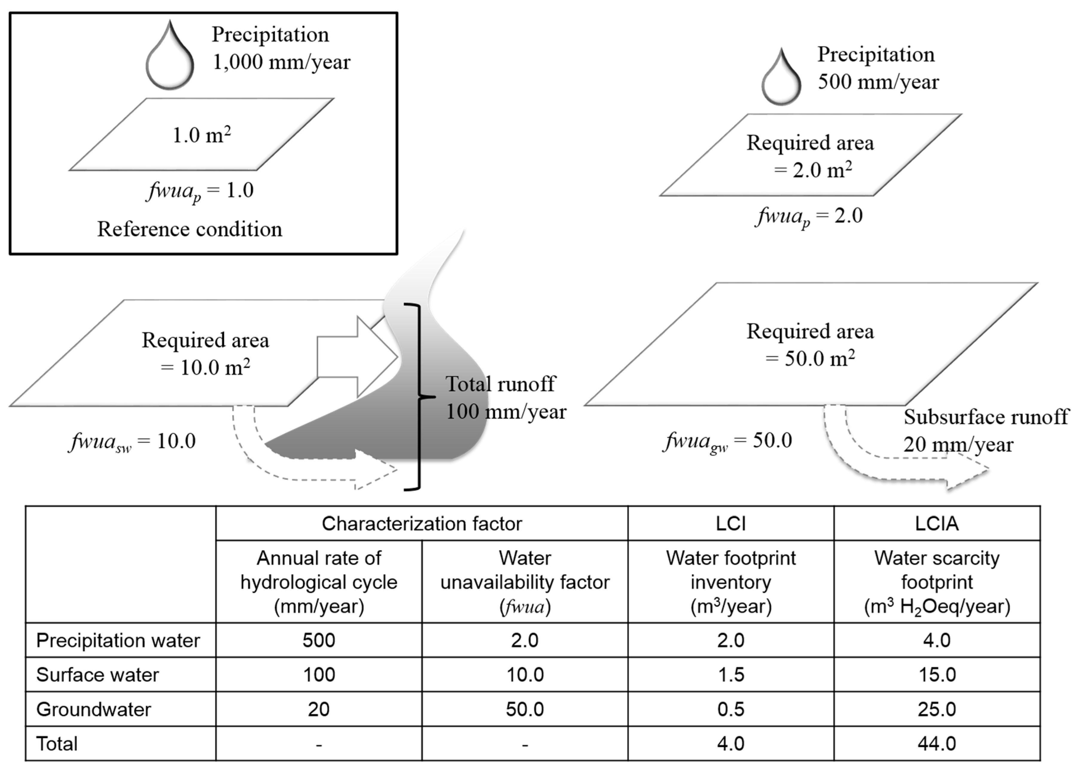
2.2. Estimating Characterization Factors

Feng et al. [42] suggested that any LCI method strongly depends on data quality. In this study, we based our calculations on a spatial resolution of 0.5 × 0.5 degrees. The characterization factor can be integrated as high-resolution grid-scale data into various spatial resolutions consistent with the data quality of the inventory, for example, at national, continental, or catchment scales. To estimate the fwua at a global, high-resolution scale that considers water sources, we used a global water resource model that provided results for terrestrial water cycle simulations.
The fwuap values were estimated from the Water and Global Change (WATCH) forcing data (WFD) [40]. The WFD provide global meteorological forcing data for the 20th century, including precipitation at a six-hourly resolution and a spatial resolution of 0.5 × 0.5 degrees. The mean annual precipitation values were extracted from the WFD for 1991–2000. The fwuap values were then estimated for each grid using Equation (1).
The H08 model [39] was used to calculate the fwuasw and fwuagw values at the global scale. H08 is an integrated model that can assess global water resources. It consists of six modules: land surface processes, rivers, crop growth, reservoirs, environmental water requirements, and coupled modules. This model makes it possible to use surface water and groundwater runoff within the natural hydrological cycle and human activities, such as reservoir operations and irrigation activities. When calculating agricultural water consumption, rainwater is the first water source used for production. When precipitation fails to meet the demands of crop growth, surface water is consumed. If surface water does not meet the demands, another water source, termed nonrenewable and nonlocal blue water (NNBW), which includes groundwater and glacial water, is used. Using this calculation process, larger WSF values will be estimated when agricultural crop growth cannot be supported solely by rainwater and cannot benefit from natural surface water, such as rivers. The precipitation input drives evaporation, total runoff, and other fluxes, which are calculated from land surface water and heat balances. The simulation setting was identical to that used previously [17], except for the meteorological forcing and calculation period. The WFD was used for meteorological forcing, and the total runoff and subsurface runoff were simulated based on the daily water demand for 1991–2000. Both local runoff at a particular location and upstream runoff are considered usable water resources; therefore, the runoff calculated for each grid was converted to the average runoff, including upstream sites, according to the flow direction in each watershed. The fwuasw and fwuagw values for each grid were estimated from the runoff calculations using Equation (1).
The calculated characterization factors of the three water sources were spatially distributed by country using national boundary data [43]. The data for each grid square was integrated into country-average values; data for fwuap, fwuasw, and fwuagw in each grid were weighted by precipitation, total runoff, and subsurface runoff, respectively. The country-average values of fwuap were calculated as:
f w u a p ¯ = l ( f w u a p , l × Q l ) l Q l = l ( Q A , r e f P l × A r e f × L l × P l ) l ( L l × P l ) = l ( L l × P r e f ) l ( L l × Q r e f ) l ( L l × P l ) l ( L l × Q r e f ) = A p , l ¯ A r e f ¯
where Ql, Pl, and Ll are the amounts of annual precipitation [m3], annual precipitation height [m], and land area [m2] at location l, respectively; and Pref is precipitation in the reference conditions [m]. The weighted value from Equation (5) is consistent with the value estimated from the country-average data. The characterization factors for rain-fed agricultural use and irrigated agricultural use were determined, and the grid square cropland area data [44,45] were used to weight precipitation, total runoff, and subsurface runoff in the rain-fed and irrigated agricultural areas. Each type of fwua was compared with other estimates calculated for 1961–1990 to validate uncertainty in the calculated characterization factors.

2.3. LCIA of the Global Virtual Water Trade

To estimate the virtual flows of WI and WSF related to the international food trade, water footprint inventories calculated for agricultural and livestock production in each country were characterized based on Equation (4). We applied the H08 model to calculate evapotranspiration for 58 commodities considering water sources, which included precipitation, stream flow, medium-sized reservoirs, and NNBW from croplands between 1991 and 2000. We adopted fwuap for WI of precipitation, fwuasw for WI of stream flow and medium-sized reservoirs, and WI of fwuagw for NNBW. At this stage, the fwua values of the 99th percentile were set as the upper limit of each distribution to avoid one extreme value from increasing the country average. The upper limit of fwuap on rainfed croplands, fwuasw on irrigated croplands, and fwuagw on irrigated croplands were 5.0, 100, and 200, respectively. The simulation setting was identical to that used for estimating the fwua. Then, virtual water flows were estimated for five major crops (barley, maize, rice, soy, and wheat) and three livestock products (beef, chicken, and pork) using the trade matrix data in 2000 [46].

3. Results

The high spatial resolution grid data of the fwua enable a detailed environmental impact assessment that reflects local characteristics. High-resolution grid-scale data can also be converted to various spatial resolutions. The fwua values are provided as gridded squares by continent or as averages by country.

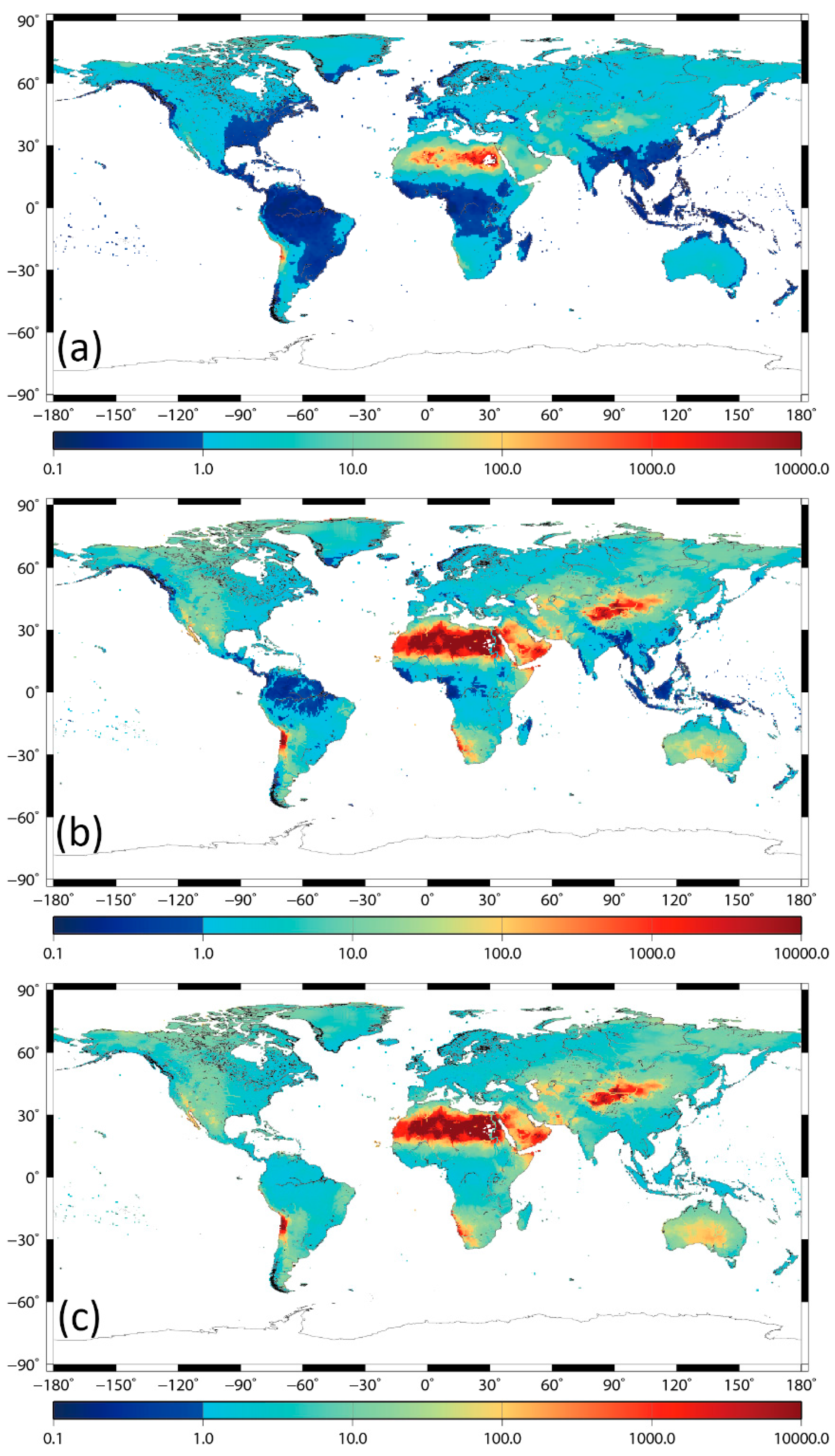
3.1. Global Distribution

The global distributions of fwua for each water source are shown in Figure 2. Values of fwuap between 10−1 and 104 accounted for 99.8% of all distributions; 99% of all distributions of fwuap were less than 600. The maximum value of fwuap, 8.5 × 10¹⁸, was found at 22.75° North and 29.25° East in Egypt. The minimum value of fwuap, 1.3 × 10⁻¹, was found at 22.25° North and 91.75° East in Bangladesh. There were areas with fwuap values less than 1.0 on all continents, mainly in South America, Central Africa, and Southeastern Asia. The fwuasw values ranged between 10−1 and 109. The maximum value of fwuasw, 3.1 × 10⁹, was found at 23.25° North and 28.25° East in Egypt. The minimum value of fwuasw, 1.4 × 10⁻¹, was found at 25.25° North and 91.75° East in China. The fwuagw values ranged between 100 and 109. The maximum value of fwuagw, 3.1 × 10⁹, was found at 23.25° North and 28.25° East in Egypt. The minimum value of fwuagw, 1.9, was found at 4.75° South and 140.75° East in Papua New Guinea. The fwuasw and fwuagw values tended to be greater than those of fwuap. Values of fwuasw and fwuagw > 1000 accounted for 5.6% of all land areas, and they were mainly distributed throughout the Sahara, Arabian Peninsula, South Africa, inland China, the Midwestern United States, and Australia.
Figure 2. Global distributions of the water unavailability factor for (a) precipitation, (b) surface water, and (c) groundwater.
Sustainability 07 09753 g002

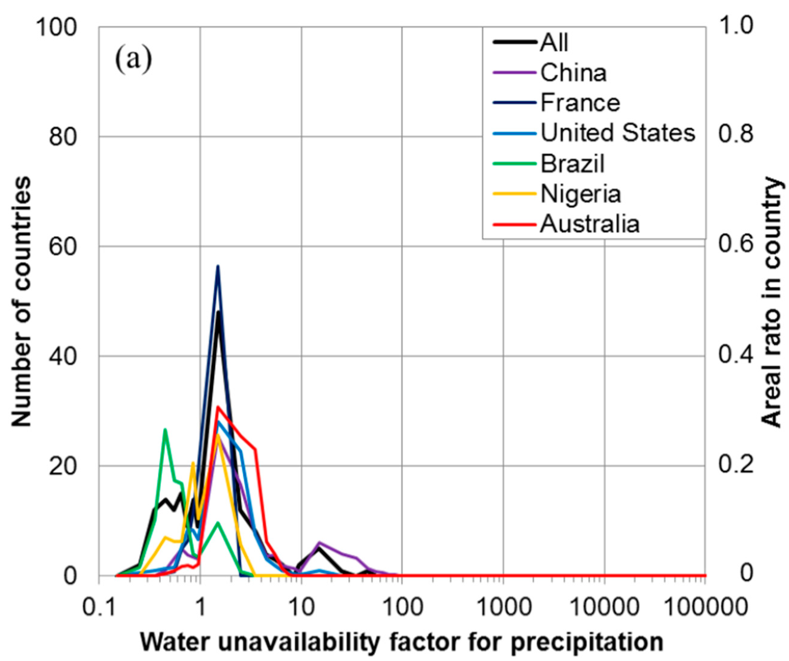
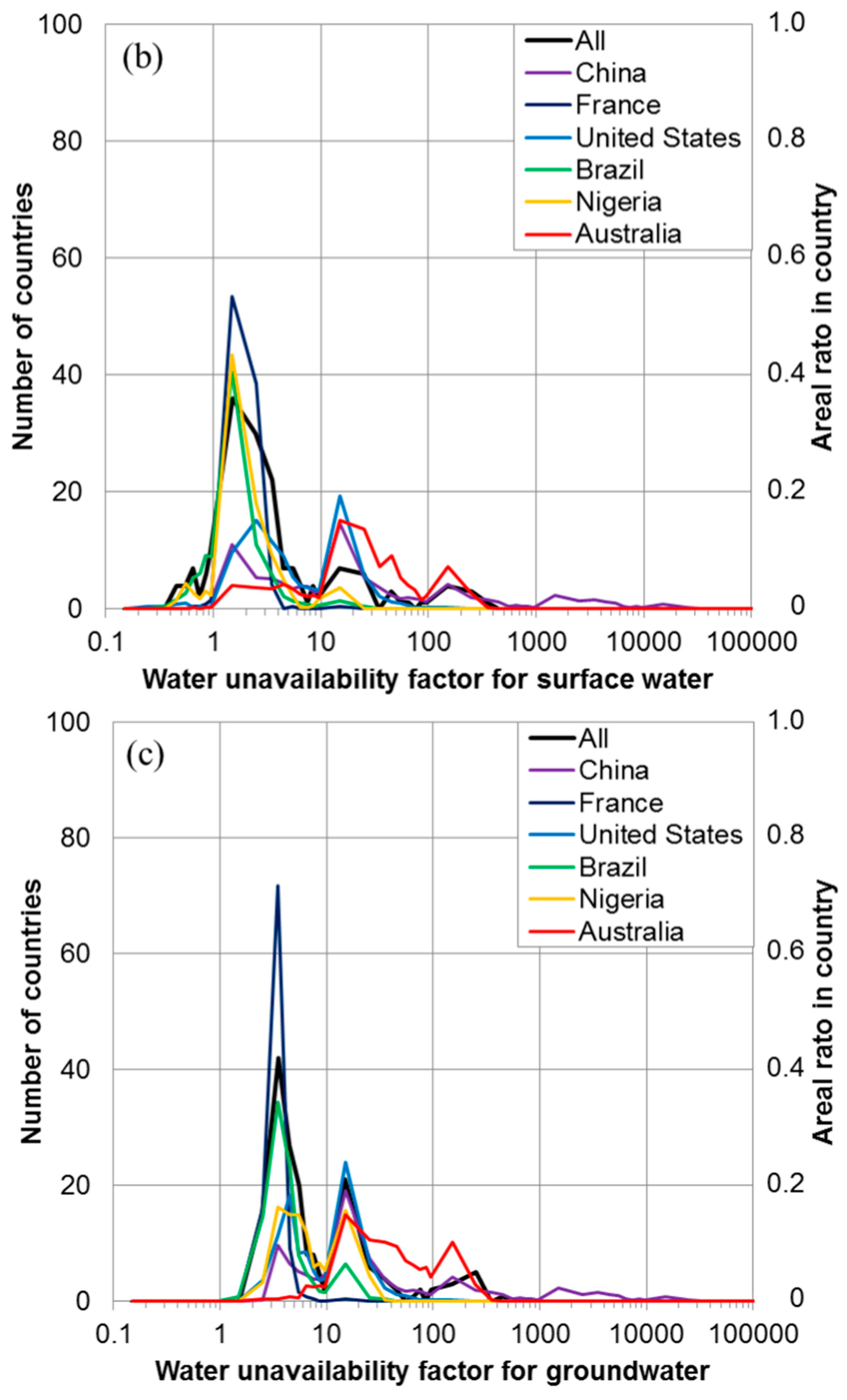
3.2. Country-Average Values

The weighted average fwua values for each water source are presented by country in Table 2 based on the entire country, rain-fed cropland, and irrigated cropland. The countries were selected from the top 25 global cereal crop producers and top 20 global commodity exporters in 2000 (FAO). Among the members of the United Nations, 153 countries with land and agricultural areas larger than one grid cell (0.5 × 0.5 degrees) are listed in the Supplementary Materials (Table S1). In Asia, Pakistan had the highest values for all types of fwua across the entire country. Indonesia, Bangladesh, Vietnam, Myanmar, and Malaysia had fwuap and fwuasw values less than 1.0 because of their high precipitation. Within Europe, all fwuap values were between 0.9 and 2.0. Spain and the Ukraine had fwuasw and fwuagw values >5.0. In North America, Mexico had higher values of fwuagw than Canada. In South America, the fwua values were smaller in Brazil due to higher precipitation. By contrast, Argentina had higher fwuasw and fwuagw values due to the arid regions in Patagonia. Egypt, which has large desert areas, had high fwua values relative to the rest of Africa. Freshwater use in such regions has a huge potential impact on its availability. The fwua value for Nigeria was lower than that of Egypt. The relatively high values in Australia can be explained by the presence of several deserts. Based on the water balance principle that water originates from rainfall, fwuap must always be smaller than fwuasw; additionally, fwuasw is equal to or smaller than fwuagw.
Table 2. Weighted-average water unavailability factor for major countries.
ContinentCountryEntire countryRainfed CroplandIrrigated Cropland
fwuapfwuaswfwuagwfwuapfwuapfwuaswfwuagw
AsiaChina1.6 4.6 10.0 1.4 1.2 3.2 7.4
India0.8 1.4 6.8 0.8 0.8 1.4 6.8
Russia2.0 4.7 6.5 1.7 1.8 4.8 6.1
Indonesia0.4 0.6 2.8 0.4 0.4 0.7 3.0
Bangladesh0.5 0.7 4.1 0.5 0.5 0.7 4.1
Vietnam0.5 0.9 4.0 0.5 0.5 0.9 4.0
Turkey1.7 4.0 6.0 1.7 1.7 4.0 6.0
Thailand0.6 1.2 4.2 0.6 0.7 1.3 4.3
Pakistan3.3 7.2 15.0 2.9 3.1 6.2 12.9
Myanmar0.5 0.6 3.9 0.5 0.5 0.7 4.0
Malaysia0.3 0.6 2.5 0.3 0.4 0.6 2.6
EuropeFrance1.0 1.8 3.4 1.0 1.0 1.8 3.4
Germany1.2 2.2 3.4 1.2 1.2 2.3 3.5
Spain1.5 3.5 6.3 1.6 1.5 3.5 6.3
United Kingdom0.9 1.6 3.4 0.9 1.1 2.1 3.8
Ukraine1.7 4.6 5.1 1.7 1.7 4.7 5.2
Poland1.5 3.3 4.0 1.5 1.5 3.3 4.0
Italy1.2 2.3 4.2 1.1 1.2 2.3 4.2
Netherlands1.1 2.1 3.4 1.1 1.1 2.1 3.4
North AmericaUnited States1.2 3.4 6.5 1.1 1.2 3.8 6.7
Canada1.7 3.6 5.8 1.3 1.3 3.0 5.3
Mexico1.2 3.6 10.9 1.2 1.3 4.0 11.6
South AmericaBrazil0.6 1.2 4.0 0.6 0.6 1.5 4.7
Argentina1.4 5.8 10.7 1.1 1.2 4.9 9.2
AfricaNigeria0.8 1.6 5.7 0.8 0.8 1.5 5.7
Egypt47.7 41.0 79.1 1985.4 23.6 12.7 24.3
OceaniaAustralia1.8 8.8 23.3 1.5 1.5 6.5 16.2
With the exception of Egypt, this principle was demonstrated in all countries. This result can be explained by the large amount of external runoff that Egypt received from an upstream country, which means that the total of the surface and subsurface runoff and the external elements exceed local precipitation. Within water-abundant countries, such as Vietnam, Thailand, France, Germany, and Brazil, there was little difference between the fwua values for the entire country and for irrigated cropland. It is assumed that agricultural lands are distributed evenly within the countries. However, the fwua values for irrigated croplands in China, Pakistan, Egypt, and Australia tended to be lower than the values for the entire country. Croplands in these countries appear to be selectively distributed in areas with sufficient water resources rather than in surrounding drier regions.
The potential impact of food production can be overestimated if it is calculated using characterization factors at a national scale. The fwua value for rain-fed croplands in Egypt was extremely high because 49 km2 of the rain-fed cropland receives only 0.5 mm of precipitation annually.

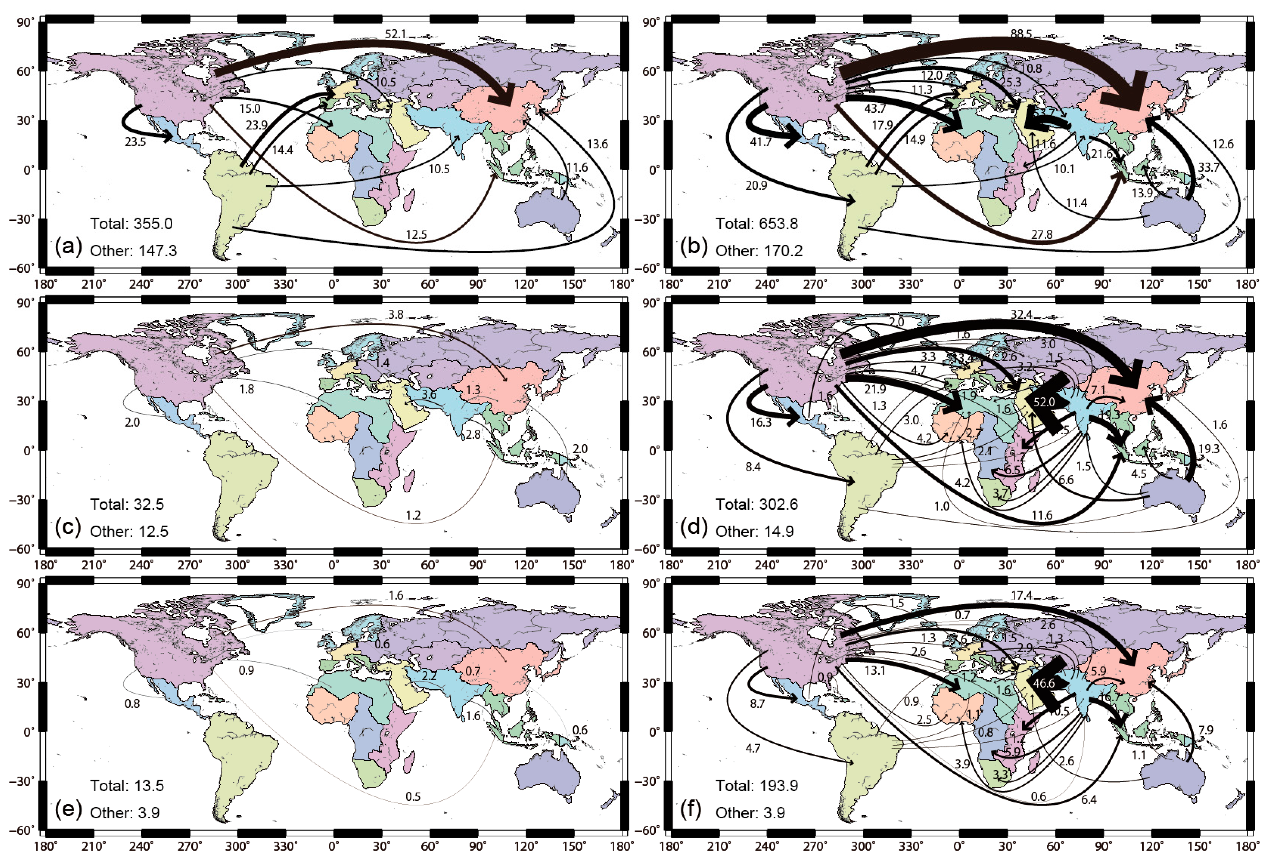
3.3. Flow of Water Footprint Inventory and Water Scarcity Footprint

In this subchapter, a case study on characterization of global virtual water trade is shown. The calculated flows of the WI and WSF by nation in 2000 were aggregated into 22 regions worldwide, based on Hanasaki et al. [17]. The net virtual exports of the water footprint inventory and water scarcity footprint for all water sources (a,d), only irrigated water including surface and NNBW (b,e), and irrigated NNBW (c,f) are shown in Figure 3. The ratio of the virtual flow of the WSF to that of the WI for each water source was 1.2 for precipitation, 5.7 for surface water, and 14.4 for NNBW. It appears that this result reflected the difference in water scarcity according to the water sources. As a remarkable characteristic, the WSF flows had greater and heavier arrows than the WI flows for all types of water. In particular, the arrows for North America, Australia and New Zealand, and Southern Asia, which were discussed as having a higher ratio of WSF to WI, were changed significantly by characterization. It is possible that agricultural activities in these areas depend on scarce water supplies. Detailed local investigations would be required to assess the sustainability of agriculture in these croplands. By contrast, flows from South America had finer lines in the impact than the inventory in Figure 4a,d. The characteristic of the lower WSF compared with WI values in this area can also be observed in the trade flows. We suggest that food production and trade from South America has relatively lower potential impacts on freshwater availability. The global virtual water flows were characterized by using the fwua for each water source. Although NNBW constituted only 3.8% of the total flow of the water footprint inventory, this increased to 29.7% of the total flow of the water scarcity footprint.
Figure 3. Virtual exports of (a) water footprint inventory for all water sources; (b) water scarcity footprint for all water sources; (c) water footprint inventory for irrigated water; (d) water scarcity footprint for irrigated water; (e) water footprint inventory for irrigated NNBW; and (f) water scarcity footprint for irrigated NNBW. Flows exceeding 10 km3/year and 10 km3 H2Oeq/year are shown in (a,b), respectively; 1.0 km3/year and 1.0 km3 H2Oeq/year in (c,d), respectively; and 0.5 km3/year and 0.5 km3 H2Oeq/year in (e,f), respectively.
Sustainability 07 09753 g003

4. Discussion

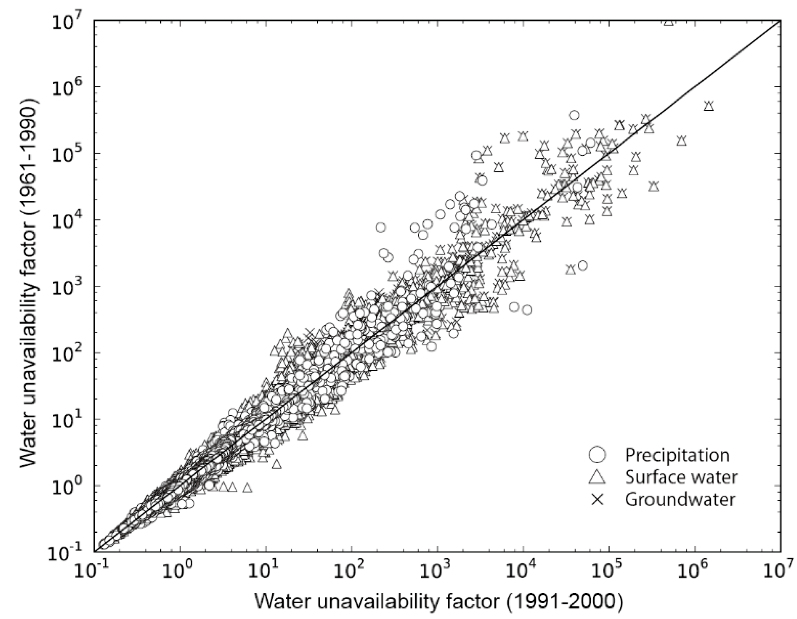
4.1. Uncertainty of Characterization Factors

To validate the variability in the fwua, we compared the fwua value of each water source for irrigated croplands for 1991–2000 and 1961–1990 (Figure 4). The total irrigated croplands had 67,420 grid cells and covered an area of 2.8 × 10⁶ km2. There was little difference between the two periods for the fwuap when the values were between 0.1 and 1.0. The largest ratio of fwuap in 1991–2000 to that in 1961–1990 (35) was found at 31.25° North and 26.75° East in Egypt. The maximum ratio of fwuasw and fwuagw in 1991–2000 to that in 1961–1990 (28) was found at 19.25° North and 20.25° East in Chad. There was greater variability in fwuasw and fwuagw than in fwuap. Runoff tends to be more sensitive than precipitation in terrestrial water cycle models [47]. These results might lead us to believe that the fwua does not vary substantially within a period of meteorological forcing. However, this may not be the case, and it is possible that the fwua varies with meteorological forcing data or model type. Validation of the uncertainty in the fwua values should be discussed.
Figure 4. Comparison of the water unavailability factor between periods.
Sustainability 07 09753 g004
To compare the spatial variability, the frequency distribution of the country-average fwua for the 153 countries and the fwua of the domestic grids in six major countries from each continent are shown in Figure 5. The fwuap in the six major countries varied from 10−1 to 102. This range was as large as that for the average between-country value. The variability between the fwuasw and fwuagw values for the major countries was larger than the variability for the average between-country values. The within-country variability is sufficiently large to suggest that it would be meaningful to prepare characterization factors at a high-resolution grid scale.
Figure 5. Frequency distributions of the water unavailability factor across 153 countries and within six major countries for (a) precipitation; (b) surface water; and (c) groundwater.
Sustainability 07 09753 g005aSustainability 07 09753 g005b

4.2. Applications in LCIAs

The functions of fwua that reflect the uneven distributions of water resources, including comparisons with existing studies, are shown in Table 3. Although the water footprint (WFN) assesses consumptive water use by water source, it is not adequate as a characterization factor for weighting water use because it does not refer to the uneven distribution of water resources. Although the water scarcity of each water source is considered in the sustainability assessment phase of water footprint (WFN), the objective explanation for simply adding the three impact indices with different references is insufficient. Because GF addresses only groundwater withdrawal, weighting of conjunctive water use is not used for assessments. The WSI shows grid-scale data that reflect the conditions in each area and considers seasonal variability using the standard deviation of precipitation as a variation factor. An increase in the stream flow due to conservation activities can be incorporated; however, this is opposed to separating surface and groundwater. The fwua proposed in this study considers the uneven distribution of water resources by location using grid-scale modeling and the effect of water conservation can be reflected by calculating the annual renewability rate of each water source. Furthermore, the fwua has an advantage over other methods by weighting the difference in water sources using a reference volume. This model can also reflect the monthly variability by increasing the temporal resolution. Characterization factors such as WSI and GF were based on the overall pressure resulting from the ratio of water withdrawal/consumption to renewability rate. On the other hand, fwua is based on renewability only and conceptually close to an initial indicator in order to be expressed by as simple a framework as possible. It can be beneficial to study the variation of the fwua distribution with/without reflecting the demand side of water use.
Table 3. Functions of the water unavailability factor and comparison with existing studies.
MethodReferenceWeighting by PlaceWeighting by TimeWeighting by SourceReflecting Effects of Conservation
Water availability factor (fwua)This studyYYYY
Water Stress Index (WSI)Pfister et al. [20]YYNY
Groundwater Footprint (GF)Gleeson et al. [23]YNNY
Water footprint (WFN)Hoekstra et al. [4]NNNN
The results of the characterization using the fwua correspond to the midpoint impact category. Kounina et al. [48] and Bayart et al. [13] showed cause-effect sequences related to water use, which lead directly from an inventory to human health protection, ecosystem quality, and resources, among other uses. We aimed to delineate a definite impact pathway of water use using an LCIA. However, there is no absolute consensus that the impact pathway of water resources should be prioritized. Characterization factors can vary within the concept of a midpoint impact assessment. Several studies that regard characterization models based on ADP [25], socioeconomic conditions [49], or energy demand [50] failed to provide an objective explanation for the reference material or impact pathways. Although the fwua is incomplete in this regard, characterization based on the required land area or collection time clearly demonstrates the differences between renewable water resources and the impacts of a unit of water consumed. The global mean precipitation can be understood intuitively as a parameter for weighting water resources, and it can easily be converted into a factor. This model can be characterized by a simpler framework compared with those already in use; it is robust and practical and is less affected by parameter uncertainty.
The methods for addressing the impacts of rainwater use on freshwater availability within an LCA are still open for debate. Milà i Canals et al. [25] indicated that rainwater use can be addressed by focusing on land use or land use change. However, it may be sensible to characterize rainwater use, particularly in agricultural fields. Rainwater, surface water, and ground water are all vital resources for agriculture. Because irrigated water from surface water or groundwater helps fill the gap between rainwater supply and the water required for growth, surface water and groundwater are alternatives for rainwater. Rainwater use involves water resources that can be diverted to other uses; thus, it can result in reduced local water availability. It is sensible to include rainwater use when explaining environmental impacts in terms of water use for crop growth. Our approach, which uses the global mean precipitation as a reference, can be more easily understood than stating multiple numbers for water use from different sources or simply summing water consumption from these sources.
The method presented here can provide characterization factors for any spatial resolution from grid cells and river basins to entire countries or continents. Additionally, this method can increase the temporal resolution of a characterization factor by setting theoretical seasonal or monthly reference conditions. This model provides various types of characterization factors based on the demands of the user. Furthermore, the fwua model should be used for actual midpoint characterizations on a global scale. This research will facilitate clarification of at-risk locations, and the magnitudes of potential impacts at the individual, product, or national level could be assessed.

5. Conclusions

A characterization model was developed to evaluate the potential impacts of water use on freshwater availability; the factor considered the uneven distribution of water resources over time, space, and source. The water unavailability factor (fwua) was defined based on the land area or collection time required to obtain a reference volume of water. In this study, the global mean precipitation was adopted as a reference volume of water. This method provides a simpler characterization framework than existing studies. The method is also robust and practical and is less affected by parameter uncertainty.
A global meteorological forcing dataset and a global water resource model were used to estimate the fwua for precipitation, surface water, and groundwater, and the fwua was calculated at a global resolution of 0.5 × 0.5 degrees based on the annual mean precipitation, total runoff, and subsurface runoff. High-resolution grid-scale data have an advantage in that they can be converted to various spatial resolutions, for example, grid cell, continent, country, or river basin. Using this method, the temporal resolution can also be increased by setting reference conditions. The fwua for precipitation tended to be smaller than that for surface and groundwater based on the water balance principle. We calculated three weighted average fwua values for each country to describe the entire country, rain-fed croplands, and irrigated croplands. The fwua of agricultural water tended to be smaller than the value for the entire country, such that the cropland areas appeared to be selectively distributed in areas with sufficient water resources rather than in surrounding drier regions. Whether rainwater use is assessed depends on the purpose of the LCIA; rainwater use reduces local water availability. We calculated characterization factors for precipitation in conjunction with those for surface and groundwater because it is important to include rainwater use for crop growth when explaining environmental impacts. We also estimated the WI and WSF flows related to international food trade. The WSF flows had greater values than the WI flows for all types of water. Although NNBW constituted only 3.8% of the total flow of the water footprint inventory, this increased to 29.7% of the total flow of the water scarcity footprint. The fwua model allows us to calculate a characterization factor that can be easily interpreted; we can also provide various types of characterization factors based on user demands. Furthermore, we can estimate the potential impacts of water use at the national, product, and individual level. We expect that this method will be incorporated into LCIA studies in the future.

Supplementary Files

Supplementary File 1

Acknowledgments

The authors thank WATCH projects and Graham Weedon for providing datasets. The data on calculated fwua for each water source are available online at http://hydro.iis.u-tokyo.ac.jp/data/WFP/. This research was supported by the Japan Society for the Promotion of Science KAKENHI, Grant-in-Aid for Scientific Research (S) (23226012).

Author Contributions

All authors contributed equally to this work. Shinjiro Yano designed and executed the model simulation, analyzed data, and wrote the manuscript. Naota Hanasaki developed analytical tools to apply the hydrological model in this work. Norihiro Itsubo gave technical support and conceptual advise based on life cycle assessment. Taikan Oki contributed conceptual thoughts of original idea and supervised this work. All authors read and approved the final manuscript.

Conflicts of Interest

The authors declare no conflicts of interest.

References

  1. Shiklomanov, I.A.; Rodda, J.C. World Water Resources at the Beginning of the 21st Century; International Hydrology Series; Cambridge University Press: Cambridge, UK, 2003. [Google Scholar]
  2. FAO. The State of the World’s Land and Water Resources for Food and Agriculture (SOLAW)—Managing Systems at Risk; Food and Agriculture Organization of the United Nations: Rome, Italy, 2011. [Google Scholar]
  3. Allen, R.G.; Pereira, L.S.; Raes, D.; Smith, M. Crop Evapotranspiration—Guidelines for Computing Crop Water Requirements; Food and Agriculture Organization of the United Nations: Rome, Italy, 1998. [Google Scholar]
  4. Hoekstra, A.Y.; Chapagain, A.K.; Aldaya, M.M.; Mekonnen, M.M. The Water Footprint Assessment Manual: Setting the Global Standard; Earthscan: London, UK, 2011. [Google Scholar]
  5. Ercin, A.E.; Aldaya, M.M.; Hoekstra, A.Y. Corporate water footprint accounting and impact assessment: The case of the water footprint of a sugar-containing carbonated beverage. Water Resour. Manag. 2011, 25, 721–741. [Google Scholar] [CrossRef]
  6. Mekonnen, M.M.; Hoekstra, A.Y. The green, blue and grey water footprint of crops and derived crop products. Hydrol. Earth Syst. Sci. 2011, 15, 1577–1600. [Google Scholar] [CrossRef]
  7. Wu, M.; Chiu, Y.; Demissie, Y. Quantifying the regional water footprint of biofuel production by incorporating hydrologic modeling. Water Resour. Res. 2012, 48, W10518. [Google Scholar] [CrossRef]
  8. Gerbens-Leenes, P.W.; Xu, L.; de Vries, G.J.; Hoekstra, A.Y. The blue water footprint and land use of biofuels from algae. Water Resour. Res. 2014, 50, 8549–8563. [Google Scholar] [CrossRef]
  9. Hoekstra, A.Y.; Chapagain, A.K.; Aldaya, M.M.; Mekonnen, M.M. Water Footprint Manual, State of the Art 2009; Water Footprint Network: Enschede, The Netherlands, 2009. [Google Scholar]
  10. Heijungs, R.; Guinée, J.B.; Huppes, G.; Lankreijer, R.M.; Udo de Haes, H.A.; Wegener Sleeswijk, A.; Ansems, A.M.M.; Eggels, P.G.; van Duin, R.; de Goede, H.P. Environmental Life Cycle Assessment of Products I: Guide—October; B&G Leiden University: Leiden, The Netherlands, 1992. [Google Scholar]
  11. Zhang, L.; Dawes, W.R.; Walker, G.R. Response of mean annual evapotranspiration to vegetation changes at catchment scale. Water Resour. Res. 2001, 37, 701–708. [Google Scholar] [CrossRef]
  12. Berger, M.; Finkbeiner, M. Methodological challenges in volumetric and impact-oriented water footprints. J. Ind. Ecol. 2013, 17, 79–89. [Google Scholar] [CrossRef]
  13. Bayart, J.B.; Bulle, C.; Deschênes, L.; Margni, M.; Pfister, S.; Vince, F.; Koehler, A. A framework for assessing off-stream freshwater use in LCA. Int. J. LCA 2010, 15, 439–453. [Google Scholar] [CrossRef]
  14. ISO. ISO 14046 Environmental Management, Water Footprint—Principles, Requirements and Guidelines; International Organization for Standardization: Geneva, Switzerland, 2014. [Google Scholar]
  15. ISO. ISO 14040 Environmental Management—Life Cycle Assessment—Principles and Framework; International Organization for Standardization: Geneva, Switzerland, 2006. [Google Scholar]
  16. Frischknecht, R.; Jungbluth, N.; Althaus, H.; Doka, G.; Dones, R.; Heck, T.; Hellweg, S.; Hischier, R.; Nemecek, T.; Rebitzer, G.; et al. The ecoinvent database: Overview and methodological framework. Int. J. LCA 2005, 10, 3–9. [Google Scholar] [CrossRef]
  17. Hanasaki, N.; Inuzuka, T.; Kanae, S.; Oki, T. An estimation of global virtual water flow and sources of water withdrawal for major crops and livestock products using a global hydrological model. J. Hydrol. 2010, 384, 232–244. [Google Scholar] [CrossRef]
  18. Pfister, S.; Bayer, P.; Koehler, A.; Hellweg, S. Environmental impacts of water use in global crop production: Hotspots and trade-offs with land use. Environ. Sci. Technol. 2011, 45, 5761–5768. [Google Scholar] [CrossRef] [PubMed]
  19. ISO. ISO 14044 Environmental Management—Life Cycle Assessment—Requirements and Guidelines; International Organization for Standardization: Geneva, Switzerland, 2006. [Google Scholar]
  20. Pfister, S.; Koehler, A.; Hellweg, S. Assessing the environmental impacts of freshwater consumption in LCA. Environ. Sci. Technol. 2009, 43, 4098–4104. [Google Scholar] [CrossRef] [PubMed]
  21. Alcamo, J.; Henrichs, T. Critical regions: A model-based estimation of world water resources sensitive to global changes. Aquat. Sci. 2002, 64, 352–362. [Google Scholar] [CrossRef]
  22. Alcamo, J.; Doll, P.; Henrichs, T.; Kaspar, F.; Lehner, B.; Rosch, T.; Siebert, S. Development and testing of the WaterGAP 2 global model of water use and availability. Hydrol. Sci. J. 2003, 48, 317–337. [Google Scholar] [CrossRef]
  23. Gleeson, T.; Wada, Y.; Bierkens, M.F.P.; van Beek, L.P.H. Water balance of global aquifers revealed by groundwater footprint. Nature 2012, 488, 197–200. [Google Scholar] [CrossRef] [PubMed]
  24. Jefferies, D.; Muñoz, I.; Hodges, J.; King, V.J.; Aldaya, M.M.; Ercin, A.E.; Milà i Canals, L.; Hoekstra, A.Y. Water Footprint and Life Cycle Assessment as approaches to assess potential impacts of products on water consumption. Key learning points from pilot studies on tea and margarine. J. Clean. Prod. 2012, 33, 155–166. [Google Scholar] [CrossRef]
  25. Milà i Canals, L.; Chenoweth, J.; Chapagain, A.; Orr, S.; Antón, A.; Clift, R. Assessing freshwater use impacts in LCA: Part I—Inventory modelling and characterisation factors for the main impact pathways. Int. J. LCA 2009, 14, 28–42. [Google Scholar] [CrossRef]
  26. Guinée, J.B.; Heijungs, R. A proposal for the definition of resource equivalency factors for use in product life-cycle assessment. Environ. Toxicol. Chem. 1995, 14, 917–925. [Google Scholar] [CrossRef]
  27. Pfister, S.; Baumann, J. Monthly characterization factors for water consumption and applica-tion to temporally explicit cereals inventory. In Proceedings of the 8th International Conference on LCA in the Agri-Food Sector, Rennes, France, 2–4 October 2012.
  28. Allan, J.A. Virtual water: A strategic resource global solutions to regional deficits. Groundwater 1998, 36, 545–546. [Google Scholar] [CrossRef]
  29. Oki, T.; Kanae, S. Global hydrological cycles and world water resources. Science 2006, 313, 1068–1072. [Google Scholar] [CrossRef] [PubMed]
  30. Yano, S.; Hanasaki, N.; Itsubo, N.; Oki, T. Characterization factors for water availability footprint considering the difference of water sources based on a global water resource model. J. LCA Jpn. 2014, 10, 327–339. [Google Scholar] [CrossRef]
  31. European Commission. Joint Research Centre—Institute for Environment and Sustainability International Reference Life Cycle Data System (ILCD) Handbook—General Guide for Life Cycle Assessment—Detailed Guidance; Publications Office of the European Union: Luxembourg, 2010. [Google Scholar]
  32. Xie, P.; Arkin, P.A. Global precipitation: A 17-year monthly analysis based on gauge observations, satellite estimates, and numerical model outputs. Bull. Am. Meteorol. Soc. 1997, 78, 2539–2558. [Google Scholar] [CrossRef]
  33. Adler, R.F.; Huffman, G.J.; Chang, A.; Ferraro, R.; Xie, P.; Janowiak, J.; Rudolf, B.; Schneider, U.; Curtis, S.; Bolvin, D.; et al. The version-2 global precipitation climatology project (GPCP) monthly precipitation analysis (1979–present). J. Hydrometeorol. 2003, 4, 1147–1167. [Google Scholar] [CrossRef]
  34. Huffman, G.J.; Adler, R.F.; Morrissey, M.; Bolvin, D.T.; Curtis, S.; Joyce, R.; McGavock, B.; Susskind, J. Global precipitation at one-degree daily resolution from multisatellite observations. J. Hydrometeorol. 2001, 2, 36–50. [Google Scholar] [CrossRef]
  35. Baumgartner, A.; Reichel, E. The World Water Balance: Mean Annual Global, Continental and Maritime Precipitation, Evaporation and Run-Off; Elsevier Scientific Publishing Company: Amsterdam, The Netherlands; New York, NY, USA, 1975. [Google Scholar]
  36. Korzun, V.I.; Sokolov, A.A.; Budyko, M.I.; Voskresensky, K.P.; Kalinin, G.P. World Water Balance and Water Resources of the Earth, Studies and Reports in Hydrology; Studies and Reports in Hydrology (UNESCO), no. 25; United Nations Educational, Scientific and Cultural Organization: Paris, France, 1978. [Google Scholar]
  37. Rudolf, B.; Beck, C.; Grieser, J.; Schneider, U. Global Precipitation Analysis Products of the GPCC; Global Precipitation Climatology Centre (GPCC); Deutscher Wetterdienst: Offenbach am Main, Germany, 2005. [Google Scholar]
  38. Dirmeyer, P.A.; Gao, X.A.; Zhao, M.; Guo, Z.C.; Oki, T.; Hanasaki, N. GSWP-2—Multimodel analysis and implications for our perception of the land surface. Bull. Am. Meteorol. Soc. 2006, 87, 1381–1397. [Google Scholar] [CrossRef]
  39. Hanasaki, N.; Kanae, S.; Oki, T.; Masuda, K.; Motoya, K.; Shirakawa, N.; Shen, Y.; Tanaka, K. An integrated model for the assessment of global water resources—Part 1: Model description and input meteorological forcing. Hydrol. Earth Syst. Sci. 2008, 12, 1007–1025. [Google Scholar] [CrossRef]
  40. Weedon, G.P.; Gomes, S.; Viterbo, P.; Shuttleworth, W.J.; Blyth, E.; Österle, H.; Adam, J.C.; Bellouin, N.; Boucher, O.; Best, M. Creation of the WATCH forcing data and Its use to assess global and regional reference crop evaporation over land during the twentieth century. J. Hydrometeorol. 2011, 12, 823–848. [Google Scholar] [CrossRef]
  41. Lvovitch, M.I. The global water balance. US IHD Bull. 1973, 23, 28–53. [Google Scholar] [CrossRef]
  42. Feng, K.; Chapagain, A.; Suh, S.; Pfister, S.; Hubacek, K. Comparison of bottom-up and top-down approaches to calculating the water footprints of nations. Econ. Syst. Res. 2011, 23, 371–385. [Google Scholar] [CrossRef]
  43. CIESIN. Gridded Population of the World Version 3 (GPWv3) Data Collection, Columbia University. Available online: http://sedac.ciesin.columbia.edu/data/collection/gpw-v3 (accessed on 1 August 2013).
  44. Ramankutty, N.; Evan, A.; Monfreda, C.; Foley, J.A. Farming the planet: 1. Geographic distribution of global agricultural lands in the year 2000. Glob. Biogeochem. Cycles 2008, 22, GB1003. [Google Scholar] [CrossRef]
  45. Siebert, S.; Doll, P.; Hoogeveen, J.; Faures, J.M.; Frenken, K.; Feick, S. Development and validation of the global map of irrigation areas. Hydrol. Earth Syst. Sci. 2005, 9, 535–547. [Google Scholar] [CrossRef]
  46. FAOSTAT. Available online: http://faostat.fao.org/ (accessed on 5 August 2014).
  47. Tang, Q.; Lettenmaier, D.P. 21st century runoff sensitivities of major global river basins. Geophys. Res. Lett. 2012, 39, L06403. [Google Scholar] [CrossRef]
  48. Kounina, A.; Margni, M.; Bayart, J.B.; Boulay, A.M.; Berger, M.; Bulle, C.; Frischknecht, R.; Koehler, A.; Milà i Canals, L.; Motoshita, M.; et al. Review of methods addressing freshwater use in life cycle inventory and impact assessment. Int. J. LCA 2013, 18, 707–721. [Google Scholar] [CrossRef]
  49. Boulay, A.M.; Bulle, C.; Bayart, J.B.; Deschenes, L.; Margni, M. Regional characterization of freshwater use in LCA: Modeling direct impacts on human health. Environ. Sci. Technol. 2011, 45, 8948–8957. [Google Scholar] [CrossRef] [PubMed]
  50. Bösch, M.E.; Hellweg, S.; Huijbregts, M.A.J.; Frischknecht, R. Applying cumulative exergy demand (CExD) indicators to the ecoinvent database. Int. J. LCA 2007, 12, 181–190. [Google Scholar] [CrossRef]

