Article

The Water Footprint of Agriculture in Duero River Basin

by
Ángel De Miguel
1,*,
Malaak Kallache
1 and
Eloy García-Calvo
1,2
1
IMDEA Water Institute, c/Punto Net 4, P.O. Box 28805, Alcalá de Henares, Madrid 28805, Spain
2
Department of Analytical Chemistry, Physical Chemistry and Chemical Engineering, University of Alcalá, P.O. Box 28805, Alcalá de Henares, Madrid 28805, Spain
*
Author to whom correspondence should be addressed.
Sustainability 2015, 7(6), 6759-6780; https://doi.org/10.3390/su7066759
Submission received: 28 February 2015 / Revised: 15 May 2015 / Accepted: 19 May 2015 / Published: 28 May 2015
(This article belongs to the Special Issue Water Footprints and Sustainable Water Allocation)

Abstract

:
The aim of this paper is to evaluate the green, blue and grey water footprint (WF) of crops in the Duero river basin. For this purpose CWUModel was developed. CWUModel is able to estimate the green and blue water consumed by crops and the water needed to assimilate the nitrogen leaching resulting from fertilizer application. The total WF of crops in the Spanish Duero river basin was simulated as 9473 Mm3/year (59% green, 20% blue and 21% grey). Cultivation of crops in rain-fed lands is responsible for 5548 Mm3/year of the WF (86% green and 14% grey), whereas the irrigated WF accounts for 3924 Mm3/year (20% green, 47% blue and 33% grey). Barley is the crop with the highest WF, with almost 37% of the total WF for the crops simulated for the basin, followed by wheat (17%). Although maize makes up 16% of the total WF of the basin, the blue and grey components comprise the 36% of the total blue and grey WF in the basin. The relevance of green water goes beyond the rain-fed production, to the extent that in long-cycle irrigated cereals it accounts for over 40% of the total water consumed. Nonetheless, blue water is a key component in agriculture, both for production and economically. The sustainability assessment shows that the current blue water consumption of crops causes a significant or severe water stress level in 2–5 months of the year. The anticipated expansion of irrigation in the coming years could hamper water management, despite the Duero being a relatively humid basin.

1. Introduction

Water use at a geographical level has traditionally been measured by indicators such as water withdrawal, which only considers the total freshwater used by a country in its production system. The use of indicators such as the water footprint (WF) allows us to analyze not only the effects generated at a national level, but all those associated with the virtual water trade [1,2]. In addition, the WF distinguishes also between blue water (irrigation from surface and groundwater) and green water (precipitation stored as soil moisture). It is, therefore, possible to quantify the impact of pollution by calculating the grey water, which is defined as the total freshwater required to assimilate the load of pollution [1]. Traditionally, this indicator has been calculated in a coarse spatial resolution using the same input values for the whole area, either on a global [3], national [4] or regional scale [5]. However, recently developed methods include the use of complex geographical models to estimate crop water use [6,7,8,9]. These models are based on a soil water balance to estimate the amount of water embedded in crops in a certain area and at a given time.
Water balance models can be developed for different time resolutions and spatial scales, thus they vary in complexity and input data [10]. There are several models to calculate crop water requirements on a global scale. Some of the most recent approaches have been implemented by Siebert and Döll [7], with a resolution of 5 min and a total of 26 crop classes (for both rain-fed and irrigated conditions). The model developed by Mekonnen and Hoekstra [6], with the same spatial resolution, was applied to 126 crops, and included grey calculations. Liu et al. [8,11] developed a model to estimate crop water use with a 30 min resolution. Since consumptive water use is defined as the total evapotranspiration of a crop during the growing period, disaggregation between blue and green water use should be performed. Therefore, the usefulness of these models goes beyond the spatial framework and high resolution, providing useful information about the green component, which is usually neglected when analyzing the agricultural sector.
The aim of this paper is to evaluate the water footprint of agriculture in the Duero river basin. To do that, we have developed the CWUModel, a spatially-explicit water balance model to assess the green and blue water consumed by crops and the water needed to assimilate the leaching of nitrogen applied as fertilizer. For this purpose, we have evaluated the green, blue and grey WF of the 19 major crops in the basin. In order to assess whether the WFs are sustainable, the monthly blue water scarcity index and the apparent water and land productivity were evaluated. The results presented in this work refer to the average WF values for the period 2003–2007.

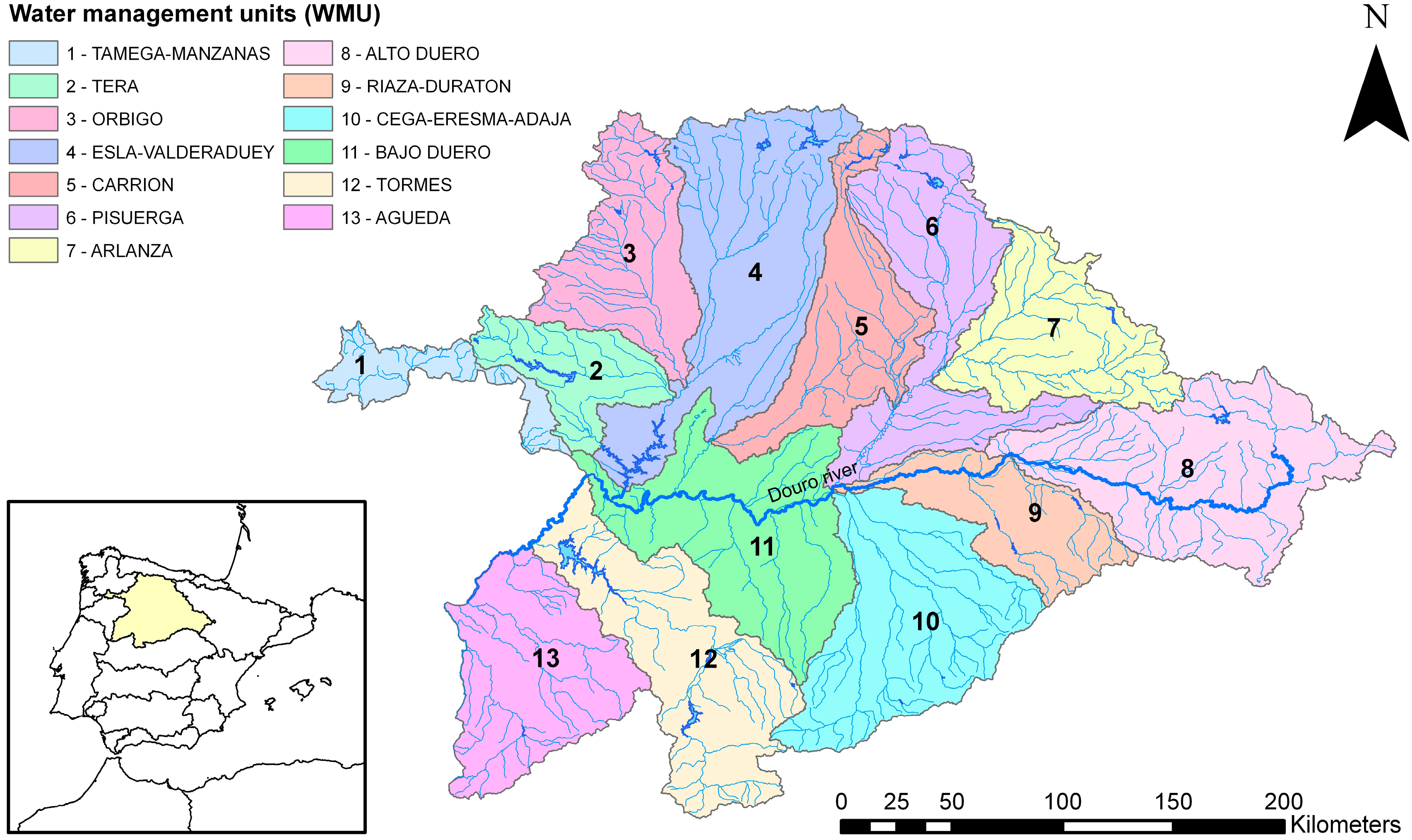
Study Area: Duero River Basin

The Duero basin is the largest river basin in the Iberian Peninsula, covering 98,073 km2 along the westward course of the Duero River and its tributaries. The river basin mostly lies in Spain (80%, 78,859 km2), but some 20% of the basin is situated in Portugal (19,214 km2). The basin has a Continental Mediterranean climate, with an average annual rainfall of 612 mm. There are significant climatic differences within the river basin. Average precipitation ranges from ca. 1800 mm in the peripheral mountain ranges to less than 400 mm in continental areas of Castile and Leon [12]. The dry period coincides with warmer temperatures while precipitation is seasonally dependent. Farmland comprises about half of the area mainly spread over the lowlands of the alluvial plains. Most crop areas, 3.5 million ha, are rain-fed while irrigated production occupies. ca. 480,000 ha. However, the gross added value of agriculture is 7%, employing 11% of the total population in the area. In any case, crops cultivated in the basin are mainly low-value-added and largely dependent on subsidies. The water resources from the basin are mainly used in agriculture (4500 Mm3/year of blue water of a total of 5000 Mm3/year used [12]). The basin is managed by the Duero River Basin Authority (DRBA) and divided into 13 water management units (WMU), each of which comprises several sub-basins (Figure 1).
Figure 1. Water management units (WMU) in the Spanish Duero river basin.
Sustainability 07 06759 g001

2. Materials and Methods

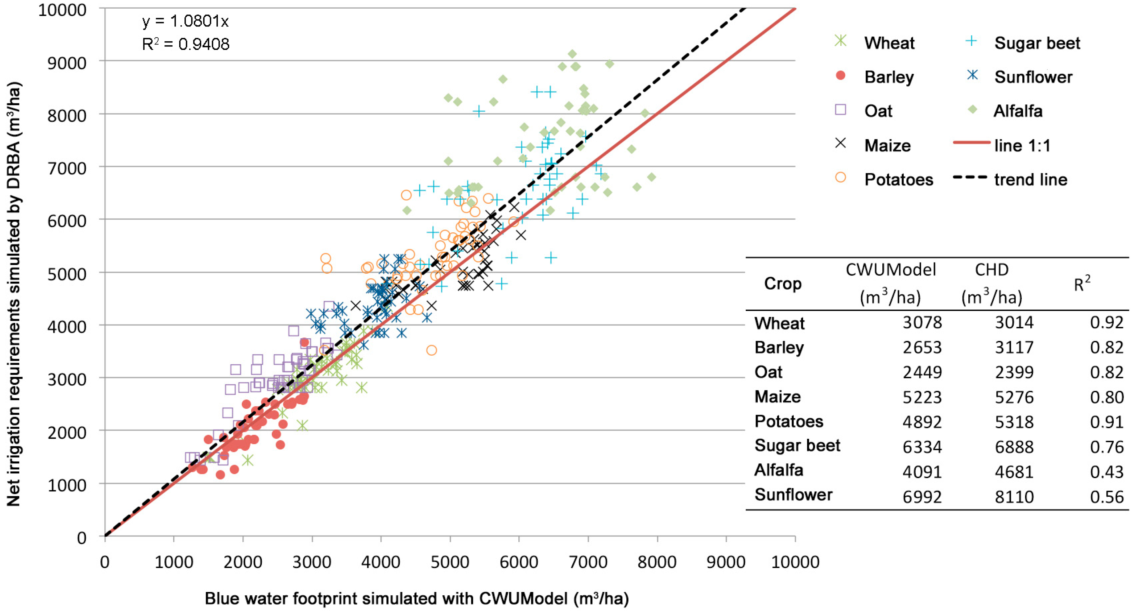
2.1. Modeling Green and Blue Water Consumption

CWUModel was developed to evaluate the green and blue water requirements of crops in the Duero river basin. The model computes in a spatially explicit way the actual evapotranspiration of the crop in non-optimal conditions following the method proposed by Allen et al. [13]. The water balance was simulated with a day-length step based on particular crop and soil features as well as on climatic variables. The model was developed using Model Builder (ESRI ArcGIS 9.3). CWUModel works on a raster format, with a high-resolution level −1 km grid size. Subsequently, the structure of the model was exported to Python in order to iterate and automate the computation. The computation was achieved taking into account the distribution of the hydrological year (October-September) in concordance with the climate of the basin [14]. The soil water balance is expressed by the following general equation (Equation (1)):
P + I = ET + R + Dp + ΔS
Here P is the rainfall (mm), I is the water input by irrigation (mm), ET is the crop evapotranspiration (mm), R is the runoff water (mm), Dp is the deep percolation under the effective root zone (mm) and ΔS is the change in the soil moisture content within the effective root zone. The soil water balance is used to simulate the ET, according to water availability in the soil and the potential evapotranspiration of the crop (ETc). In our case, we have simulated the crop evapotranspiration under non-standard conditions (ETcadj) in line with Allen et al. [13] (Equation (2)):
ETcadj = Kc × Ks × ET0
where Kc is the crop coefficient and Ks is the water stress coefficient, both of them specific for each crop, and ET0 is the reference evapotranspiration (mm). Kc varies with time, as a function of the plant growth stage. The parameters needed to produce the daily Kc curve are obtained from Allen et al. [13]. Daily Kc is computed by linear interpolation between the tabulated values of Kc at the different growth stages (initial, development, mid-season and late-season stages) using the number of days the crop spends in each period. The planting date and cropping season were obtained from MAPYA [15] and from the Castile and Leon irrigation department. Kc values for the mid and late seasons were subsequently adjusted to the local climate conditions [13] (Equation (3)):
K c a d j = K c T a b + [ 0.004 × ( u 2 2 ) 0.004 × ( R H min 45 ) ] × ( h 3 ) 0.3
where Kcadj is the adjusted crop coefficient, KcTab is the tabulated crop coefficient, u2 is the average wind speed at two meters above ground level (m/s), RHmin is the average daily minimum relative humidity (%) and h is the crop height (m). Kc was adjusted for each year throughout the basin using the climate information from 38 weather stations [16].
Ks is introduced to account for the effect of water stress on crop transpiration. Ks depends on the available soil water and is computed according to Allen et al. [13] (Equation (4)):
K s = { 1 o t h e r w i s e S ( 1 p ) × S max i f   S < ( 1 p ) × S max
where S is the actual soil moisture (mm), Smax is the maximum moisture a soil can hold (mm) and p is the crop depletion factor. Smax is a function of the total available water capacity (TAWC) of a soil (mm/m) and the respective crop root depth (m). The factor p is specific for each crop and refers to the amount of water a crop can extract from the soil without suffering water stress. This was computed according to Allen et al. [13].
TAWC grid-based data at 1 km resolution were obtained from the ESDB database [17]. Across the soil profile, two horizons are identified: deep and superficial (up to 20 cm deep). Smax was computed by multiplying TAWC values by the depth of the crop root. Where the root depth had a higher value than the maximum soil depth, the latter was used to calculate Smax. In addition, different root depth values were used for rain-fed and irrigated crops [18].
Monthly ETo and P were obtained from the SIMPA grid database [19], which offers monthly climatic information at 1 km resolution for the period 1940–2010. SIMPA is a hydrological model where ETo is obtained by combining the Thornthwaite and Penman-Monteith methods. Monthly ETo was rescaled to daily estimates of ETo by means of linear interpolation as suggested by Mekonnen and Hoekstra [6].
Stochastic weather generators are commonly used to obtain daily P. They generate daily data series avoiding the problems related to the lack of data [20]. Although different global data sets comprise the information needed for the generation of daily climatic data, their spatial resolution is usually too high to apply them directly to a regional analysis. Therefore, we developed a stochastic daily generator based on a study by Castelví et al. [21] to generate daily precipitation from the gridded monthly precipitation data in the SIMPA model. The process of generation of daily data is based on two steps: firstly, the occurrence of wet days is estimated; then the precipitation volume for each wet day is derived. The model was calibrated using daily climatic data from 38 agroclimatic stations [16]. A complete description can be found in De Miguel et al. [22].
Since not all the precipitation infiltrates the soil to become available to the plants, the amount of rainfall lost through runoff (R) has to be computed. We used the equation proposed by Liden and Harlin [23] (Equation (5)):
R = ( P + I ) × ( S S max ) γ r
where I (mm) is irrigation water and the parameter γr is correlated with the runoff intensity. We used a fixed value of 2 for rain-fed cultures and 3 for irrigation following Siebert and Döll [7].
The water balance is calculated for irrigated and rain-fed crops separately. For rain-fed crops, the consumptive use of green water is obtained as the sum of the daily actual evapotranspiration, where precipitation is the only water supply (Equation (1)). In the case of irrigated crops, blue water consumption was calculated by performing two different soil water balances scenarios [1]. The first scenario computes the green water consumption in the same way as for rain-fed crops, but using crop parameters for irrigated crops. The second one simulates the soil water balance so that the irrigation requirement is always met (full irrigation). Since not all the irrigation requirements of the crops are always met in the basin (deficit irrigation), the water supply security factor (WSS), defined as the fraction of water demand provided by each irrigated area under normal conditions (variable between 0.9–1), was used [12]. Therefore the blue water footprint was obtained by multiplying the irrigation requirements of the crop in a specific area (second scenario) by the WSS of this irrigated area, minus the green water consumption as estimated in the first scenario. The water balances are computed for the whole year. A constant Kc of 0.3 before the planting date is used in order to define initial soil moisture.

2.2. Modeling the Nitrogen Leaching and Grey Water Footprint

CWUModel is also able to estimate the grey WF of crops, defined as the total freshwater needed to assimilate the nitrogen leached. The methodology proposed by Hoekstra et al. [1] was used (Equation (6)) to simulate it:
W F g r e y = N L e a c h i n g C max C n a t
where NLeaching is the amount of nitrogen leaching from the soil (mg/L), Cmax is the maximum allowed concentration of nitrogen in the receiving water, established as 50 mg/L of nitrate in groundwater bodies [24] and Cnat is the natural nitrogen concentration assumed to be 0.5 mg/L as other authors have proposed [25,26]. NLeaching was computed according to the model proposed by De Willegen [27] (Equation (7)):
N L e a c h i n g = ( 0.0463 + 0.0037 × P C × L ) × ( F + D + N O M U )
where P is the annual precipitation (mm), C is the clay soil content (%) obtained from the ESDB database [17], and L is the crop root depth (m). F is the nitrogen rate application (kg/ha), D is the annual decomposition rate, established as 1.6% as recommended by the FAO [28], NOM is the amount of nitrogen in soil organic matter (kg/ha) and U is the nitrogen uptake by crops (kg/ha). For irrigated crops, we add the gross irrigation requirement of the crop to the amount of rainfall. The values for the previous variables in the river basin are within the boundaries of the regression model, established as 40–2000 mm of rainfall, 3%–54% clay content and 0.25–2 m layer thickness.
F was obtained from the “Nitrogen balance in Spanish agriculture” [29], where disaggregated values of organic and mineral N rates could be found for each crop and management system at provincial level. Following the methodology used in the annual balance, U was also calculated as a function of the crop yield, using the nitrogen extraction coefficients (Ce). In the case of NOM, the HWSD soil database was used [30].

2.3. Harvested Areas

Grid-based maps of growing areas for the 5 major cereals in the Duero river basin were developed, distinguishing between irrigated and rain-fed managements. They were created based on the SIOSE land use map [31]. SIOSE provides information on land use for the year 2005 and is into 90 categories, of which 12 belong to arable areas. With a 1:25,000 scale, the crop distribution was extracted and transformed into a 1 km grid-based data. Major crop categories were distributed into specific crops by combining crops coverage with two statistical data sources featuring different geographical and temporal resolution [32,33]. We assumed that each pixel belonging to a crop group in a particular area is proportionately composed of all those crops listed among the statistical information.

2.4. Sustainability Assessment

To assess whether the WFs relating to crops are sustainable, we identified the monthly blue water scarcity index (BWS) as proposed by Hoekstra et al. [34]. BWS is defined as the ratio of the total blue WF to the blue water availability within a certain period, the latter being the natural runoff (Rnat) minus the environmental flow requirement (EF). BWS is classified into four levels: low (<1), moderate (1–1.5), significant (1.5–2) and severe (>2) water scarcity, and indicates the number of months the WF exceeds water availability. Since there is no gauging station at the end of the Spanish river basin, the BWS was calculated in three different areas covering over 95% of the irrigation areas and with minimal water transfer infrastructures: A66 (Duero River, total surface of 46,170 km2); A88 (Tormes River, total surface of 4650 km2); A95 (Esla River, total surface of 14,430 km2) (see Figure S1).
A proper definition of EF is essential to establish how much water is unavailable for use, so two situations were assumed: (i) we have use the minimal EF defined by the DRBA [12] based on hydrobiological aspects (EFeco) and (ii) the “presumptive environmental flow standard” as proposed by Richter et al. [35] established as 80% of the natural runoff (EFstd). Both natural runoff and stream runoff were also obtained from the DRBA [12].
Since BWS considers all the blue water consumption in a certain area, the blue WFs of urban areas, industry and livestock were also considered. For the first, a balance between blue water abstraction and discharge was developed. For the remainder, we assume a consumption rate of 10% [36]. Evaporation from reservoirs is another issue. It has been calculated from the ratio between the stored volume and flooded area established by DRBA [12] for reference dams. As pointed out in the river basin management plan [12], a drastically increase in the irrigated areas is expected in the comming years, so BWS is also evaluated for the planning horizons 2015 and 2027.
The sustainability assessment was refined by including an economic analysis, evaluating the apparent water and land productivity (AWP and ALP respectively) as proposed by Garrido et al. [37]. The former is defined as the ratio between the market price of the crop and its WF (green and blue component), and the latter as the ratio between the market price of the crop and its yield.

3. Results

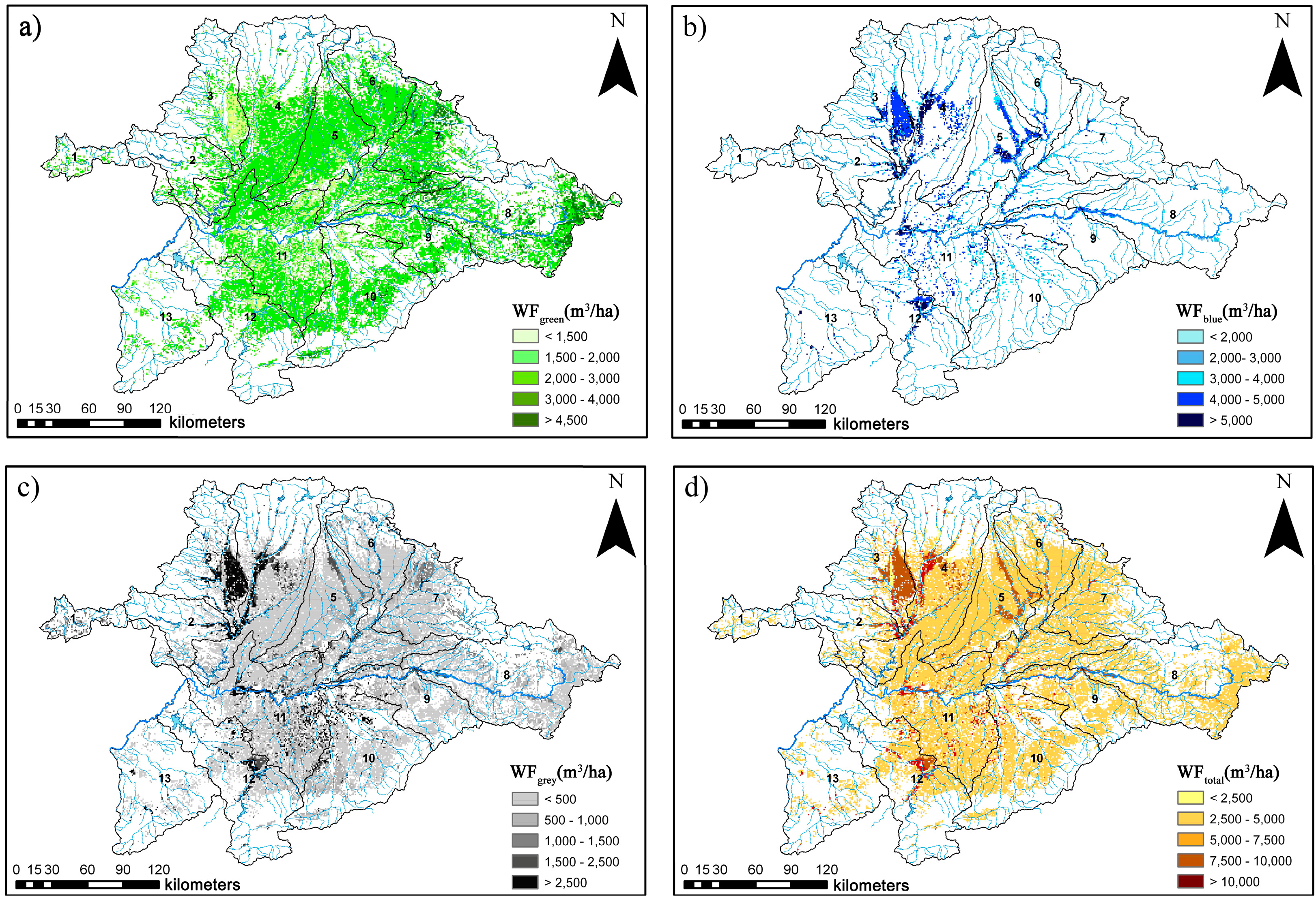
3.1. The Total Green, Blue and Grey Water Footprint of Crops

With a total harvested area of 2.6 million ha, the WF of crops in the Duero river basin over the 2003–2007 period is established at 9473 Mm3/year (59% green, 19% blue and 21% grey) of which 5548 Mm3/year (86% green and 14% grey) correspond to the 2.2 million ha cropped in rain-fed, and 3924 Mm3/year (20% green, 47% blue and 33% grey) in irrigated lands (Table 1).
Table 1. Harvested area, production and WFgreen, WFblue and WFgrey for the major crops in the Duero river basin, average values for the period 2003–2007. Values for all the crops can be found in Table S1.
CropsSystemSurface (ha)Production (1000 tons)WFgreen
(1000 m3)
WFblue
(1000 m3)
WFgrey
(1000 m3)
WFTotal
(1000 m3)
CerealsRainfed1,743,42547204,095,7320703,9994,799,731
Irrigated290,1052024538,5451,129,254815,7622,483,561
LegumesRainfed174,728158280,63303146283,778
Irrigated15,9632919,27811,45874131,477
PotatoesRainfed1295262236057157951
Irrigated19,75377926,85094,557200,513321,920
Industrial cropsRainfed143,233158255,2140764255,978
Irrigated63,4253,714112,614356,327200,308669,248
ForageRainfed57,6181045130,46203093133,555
Irrigated32,125173082,754222,6361608306,998
VegetablesRainfed000000
Irrigated883230211,28836,81960,747108,854
VineyardsRainfed58,55823661,0070787867,211
Irrigated2299151145131512052921
Total Rainfed2,178,85763424,825,2850724,5945,548,205
Irrigated432,5028593792,4741,852,3651,280,8833,924,979
Total2,611,35914,9355,617,7601,852,3652,005,4789,473,184
Cereals are by far the most common crops in the Duero river basin. Cultivation of cereals in rain-fed lands is responsible for 4799 Mm3/year of WF (85% green and 15% grey), whereas the irrigated WF comprises 2483 Mm3/year (22% green, 45% blue and 33% grey). Barley is the cereal with the highest WF, with almost 3512 Mm3/year (76% green, 8% blue and 16% grey), followed by wheat, with a total WF of 1646 Mm3/year (82% green, 8% blue and 10% grey) and maize, with a total WF of 1626 Mm3/year (14% green, 41% blue and 45% grey) (see Table S1). Other crops of note are the industrial crops (sugar beet and sunflower) with a WF of 925 Mm3/year (39% green, 39% blue and 22% grey), forage with a WF of almost 440 Mm3/year (48% green, 50% blue and 2% grey) and potatoes with a WF of 329 Mm3/year (9% green, 29% blue and 62% grey).
The average WF is 3628 m3/ha, although there are large differences between rain-fed and irrigated areas. The former has an average WF of 2546 m3/ha, whereas the latter has a WF of 9075 m3/ha. This effect can be clearly seen in Figure 2. The darker areas are those with a more intensive freshwater appropriation, corresponding generally to crops in an irrigation system. The high blue water consumption (Figure 2b) is linked to higher impacts due to the use of nitrogen in fertilizer (Figure 2c), resulting from the intensification of land use. In the case of green water (Figure 2a), irrigated crops with a poor root system development have the lowest consumption.
Figure 2. (a) Green; (b) blue; (c) grey and (d) total WF of cereals in the Spanish Duero river basin, average values for the period 2003–2007. Data are shown in m3/ha and account for all the cereals presented in each grid cell. A summary of the water footprint per WMU can be found in Table S2.
Sustainability 07 06759 g002

3.2. Blue Water Use, Consumption and Source

The majority of consumed blue water (63%) comes from surface water bodies, being surface and sprinkler irrigation the prevailing technology in the area. Although the simulated surface water consumption of crops is 1163 Mm3/year, the total water abstracted is computed as 2349 Mm3/year. A large amount of the water is lost in the application process (46%), while the remaining 54% is lost during transport and distribution. Groundwater consumption is computed as 688 Mm3/year whereas the total groundwater abstracted is simulated as 917 Mm3/year. Water losses are minimized in groundwater management, since distribution and transport infrastructures are not required. Furthermore, sprinkler irrigation is the predominant system, since pressure is needed to extract water from the aquifer. This entails extracting 25% more of water than that consumed by crops when farms are irrigated with groundwater. This volume is as high as 47% for lands irrigated with surface water (see Table S3).

3.3. Grey Water Footprint of Nitrogen Application as Fertilizer

Due to the 230 thousand tons of nitrogen applied to crops, the estimated grey WF is simulated as 2005 Mm3/year (Table 2). Crops are able to extract around 84% of the total nitrogen applied, while 10% is leached. The average nitrogen application is estimated as 94 kg/ha, although large differences can be found for different crops and management systems. While wheat cropped in irrigated lands is fertilized with 110 kg/ha, maize receives 423 kg/ha. Despite the large nitrogen requirements of crops managed under irrigated farming, the water needed to assimilate the leaching of nitrogen is computed as 2962 m3/ha, almost seven times greater than for crops in rain-fed conditions (333 m3/ha). Crops such as maize, sugar beet and potatoes present a WFgrey per area of 5703 m3/ha, 4362 m3/ha and 10,151 m3/ha respectively (see Table S4).
Table 2. Application, crop extraction, leaching and WFgrey of nitrogen used as fertilizer in the Duero river basin, average values for the 2003–2007 period.
CropsSystemN Application (tons)N Extract by Crops (tons)N Leached (tons)WFgreyWFgreyWFgrey 10%
(1000 m3)(m3/ha)(1000 m3)
CerealsRain-fed119,94696,0917596703,9994041,111,645
Irrigated71,00942,6238802815,7622812658,100
LegumesRain-fed131974673431461812,221
Irrigated81512368741467553
PotatoesRain-fed29311762571544142713
Irrigated791242102164200,51310,15173,328
Industrial cropsRain-fed10765353876459976
Irrigated19,24115,3722161200,3083158178,319
ForageRain-fed8774801333093548130
Irrigated110792341716085010,261
VegetablesRain-fed00000
Irrigated2567173665560,747687823,794
VineyardsRain-fed89712018578781358313
Irrigated182751312055241687
Total Rain-fed124,409115,0307818724,5943331,152,999
Irrigated102,83374,48513,8211,280,8832962953,042
Total227,242189,51521,6392,005,4787682,106,041
Furthermore, we have developed a grey WF analysis using the traditional assumption that 10% of the total nitrogen applied is lost through leaching and or runoff [6,38] (Table 2). We can see that the WFgrey is estimated at 2106 Mm3/year, 5% higher than the values computed by CWUModel. However, a detailed analysis shows significant differences between cropping systems. Since data modeled with CWUModel establishes a WFgrey of 724 Mm3/year for rain-fed crops and 1280 Mm3/year for irrigated crops, the simulation developed under the assumption of 10% estimate a WFgrey of 1152 Mm3/year and 953 Mm3/year respectively. This is because rain-fed crops in the basin present a lower application rate and high productivity; thus, the total nitrogen leached is limited to 6% of the total nitrogen applied. In contrast, irrigated cropping, despite the high yields, is unable to extract high application rates, which combined with high soil moisture and limited rooting depth, increases the leaching of the mobile nitrogen, totaling in 14% of the overall nitrogen applied (varying from 12%–31% depending on the crop).

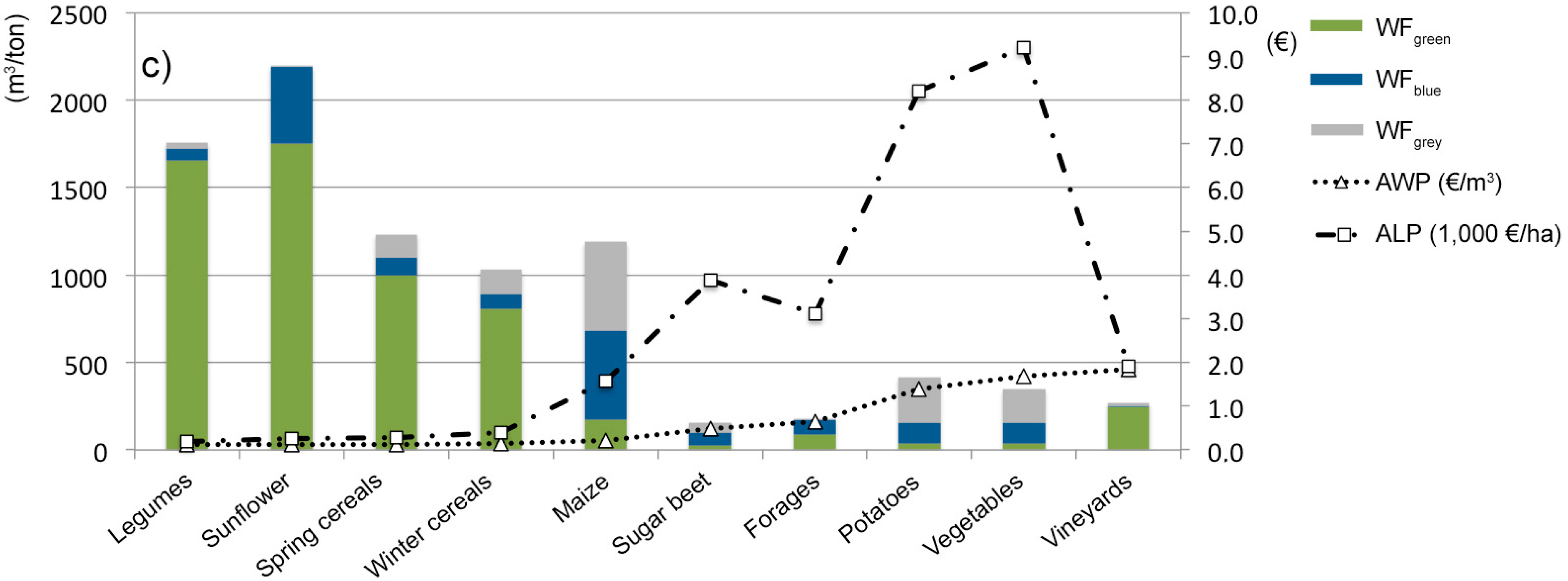
3.4. Water Footprint per Ton of Product

With an average yield of 5613 kg/ha, the WF per ton in the Duero river basin is 646 m3/ton (918 m3/ton in rain-fed and 468 m3/ton in irrigated). This is because the crops commonly planted in the irrigated areas present a higher yield than those cropped in rainfed areas (maize, sugar beet, potatoes, forage and vegetables). The sunflower is the crop with the highest WF, with an average value of 2199 m3/ton followed by vetch and ray, with a WF of 2132 and 1129 m3/ton, respectively. Cereals present relatively homogeneous values, with a WF around 900–1100 m3/ton, except in the case of maize whose average value is simulated as 688 m3/ton. Other crops such as sugar beet or potatoes present a WF of 157 and 412 m3/ton respectively (see Table S5).
Nevertheless, some differences were found related to the cropping system. For the majority of the crops, the values simulated in rain-fed conditions are lower than those in irrigated. For example, we have computed a WF of 968 m3/ton for wheat in rain-fed while this value rises to 1104 m3/ton in irrigated. Crop water productivity (CWP) was also evaluated (disregarding WFgrey): a slightly higher CWP was found for most of the crops in rainfed conditions, especially for winter cereals.

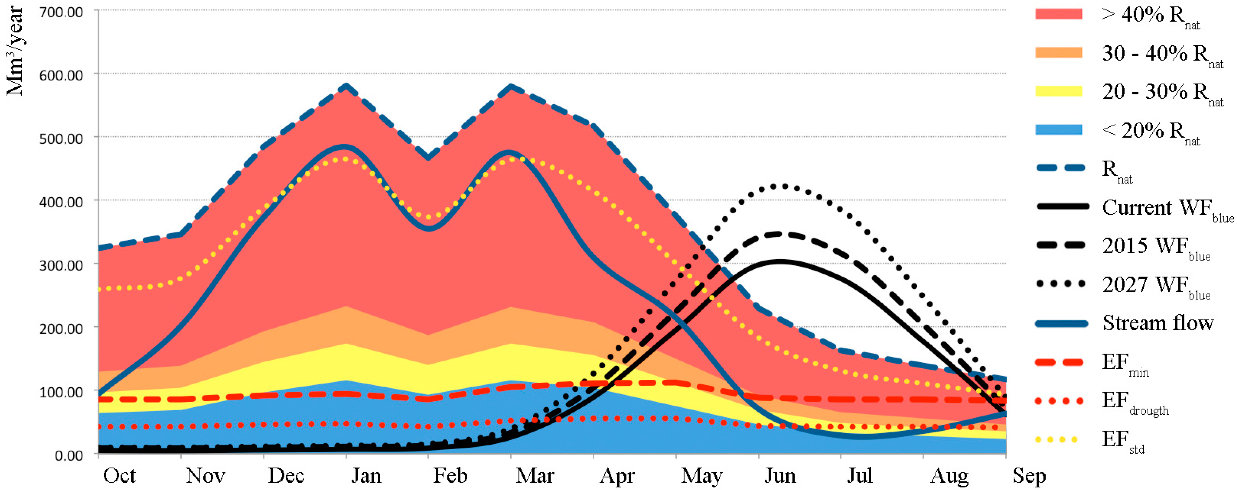
3.5. Sustainability of the Blue Water Footprint

With a WFblue simulated at 1155 Mm3/year (92.0% agriculture, 3.5% dam evaporation, 3.8% urban, 0.5% livestock and 0.2% industrial) in A66, 130 Mm3/year (80.4% agriculture, 13.0% dam evaporation, 6.0% urban, 0.4% livestock and 0.2% industrial) in A88 and 678 Mm3/year (93.5% agriculture, 4.7% dam evaporation, 1.5% urban, 0.1% livestock and 0.2% industrial) in A95, the number of months in which the river basin suffers water scarcity varies between 2 and 5 according to the drainage basin and the EF assumed. Thus, if we consider the EFeco, the number of months with blue water scarcity is simulated at 3 (1 moderate and 2 severe) for A66, 2 (severe) for A95 and also 2 (moderate) for A88. These results vary considerably if we consider the EFstd, with 5 months of blue water scarcity for A66 (1 moderate and 4 severe), 4 months for A95 (1 significant and 3 severe) and 3 for A88 (severe) (Table 3). The expansion of irrigated areas expected in the coming years translates into an increment in the number of months with significant and severe water scarcity.
Table 3. Number of months in which drainage basin suffers blue water stress, average values for the 2003–2007 period and for the planning horizons 2015 and 2027. The relation between Rnat and WFblue is also shown.
Drainage BasinPeriodLow StressModerate StressSignificant StressSevere StressBlue Water Scarcity Index Annual Monthly Average ValueRelation Rnat/WFblue (%)
EFstdEFecoEFstdEFecoEFstdEFecoEFstdEFecoEFstdEFeco
A95Current8100010321.560.5914.2%
2015780111422.861.0826.1%
2027780012423.161.2028.8%
A66Current791100421.910.6725.9%
2015692100422.220.7730.2%
2027691010432.700.9436.7%
A88Current9100200301.000.2911.8%
2015791110322.190.6326.0%
2027791100422.810.8033.3%
As we can see in Figure 3, blue water scarcity in A66 occurs during the summer months, where the blue water demand is highest and Rnat is at its lowest values. In these months the water supply is guaranteed through reservoirs and groundwater abstraction, allowing WFblue to be higher than Rnat for at least three months per year. However, this results in the stream flow being greatly diminished—in some periods lower than the EFeco. A similar pattern was found in A88 and A95 (see Figure S2), although in these cases the stream flow is always higher than EFeco. Thus, the average monthly stream flow entailed 54%, 76% and 88% of Rnat for A66, A88 and A95, respectively.
Figure 3. Blue water scarcity index of for drainage basin A66 for the simulated period (average 2003–2007) and for the planning horizons 2015 and 2027. Figures for A88 and A95 can be found in Figure S2.
Sustainability 07 06759 g003

3.6. Apparent Water and Land Productivity

The LAP for irrigated areas is higher than that obtained for rain-fed conditions, with an average LAP of 2156 €/ha compared to 425 €/ha. While irrigated agriculture only comprised 16% of the total harvested area, the value of the crops accounts for 50% of the total. Significant differences were found between crops: an average LAP above 8000 €/ha for vegetables or potatoes compared to an average LAP below 500 €/ha in the case of cereals. The Duero river basin is characterized by low productivity crops, with an average APW of 0.24 €/m3. As we can observe in Figure 4, the crops with the lowest AWP are those with the highest WF per ton, such as legumes, sunflower or cereals. In contrast, those with the lowest WF present a relatively high economic yield (high AWP and ALP), such as sugar beet (0.48 €/m3), forages (0.82 €/m3) or potatoes (1.78 €/m3). Vines are also noteworthy, with an average AWP of 2.8 €/m3 and a WF of 261 m3/ton (94% green, 1% blue and 5% grey) as the crop with the highest AWP.
Figure 4. Water footprint per ton, apparent water productivity (€/m3) and apparent land productivity (€/ha) for major crops in the Duero river basin, average values for 2003–2007 period.
Sustainability 07 06759 g004

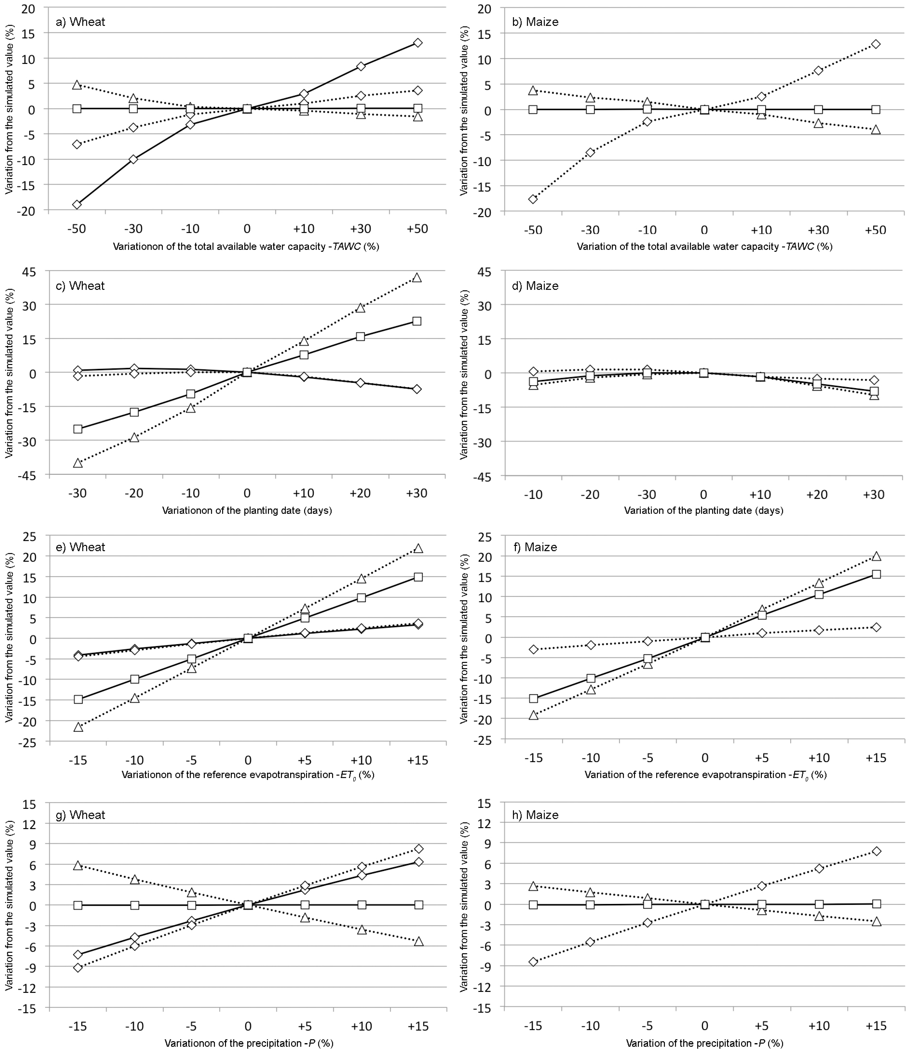
3.7. Sensitivity Analysis

We tested the effect that changes in four parameters have on green and blue WF values: TAWC, planting date, ET0 and p. The first two were selected as per suggestion of other authors [6,7]. The latter two were selected in order to test the dependence of the model on the input climatic data. This was achieved by varying the input values for the WF of wheat and maize: TAWC (±10%, ±30% and ±50%); planting date (±10, ±20 and ±30 days); and ET0 and p (±5%, 10% and ±15%). We performed the calculations for the year 2004, distinguishing between rain-fed and irrigated farming in the case of wheat and irrigated farming for of maize.
For TAWC (Figure 5a,b), major differences were found for rain-fed cereals, where we detected an increase of 15% in the total crop water consumption when we varied the TAWC by 30%. In the case of irrigated land, the total crop water use remains relatively constant, with variations in green and blue water of under 5% with a variation of 30% in the TAWC. In both cases, increments in the soil holding capacity cause an increase in the green component.
Figure 5. Variation of the green and blue water consumption regarding the variation of the TAWC (a,b); planting date (c,d); ET0 (e,f); P (g,h).
Sustainability 07 06759 g005
In terms of planting dates (Figure 5c,d), different patterns were found between wheat and maize, especially in irrigated farming. Wheat shows a significant increment in blue water demand, up to 50% higher values when we delay the planting date by 30 days. In the case of maize, the increment in the WF is negligible. This is because wheat is a long-cycle cereal and therefore a delay in the planting date causes a significant water demand in the warmer and driest months.
Extensive changes could be detected for irrigated crops in ET0 (Figure 5e,f). A variation of 15% of the ET0 results in an increment of the blue water demand of around 20%. In contrast, changes in the variable p (Figure 5g,h) particularly affect the simulations of crops managed in rain-fed condition. Thus, a 15% change in p translates into a variation of 10% in the green component.

4. Discussion

4.1. Comparison with Other Regional and Global Studies

The blue water requirement of crops was compared with the net irrigation requirements estimated by the DRBA [12] for the different agricultural regions. The results correlate well with a R2 of 0.951 (Figure 6). Despite similar methodology being used, differences in blue water demand for each cereal could be noted. These differences result from: (i) the estimation of net irrigation necessities by the DRBA is calculated as the difference between the ETc and precipitation, assuming negligible runoff; (ii) the coarse spatial resolution used by the DRBA, with climatic and soil information defined according to a proximity criterion; (iii) differences in crop variables for some crops.
The results were also compared with data modeled by Mekonnen and Hoekstra [6] and Siebert and Döll [7] in their global studies for the same crops and area (only for blue and green WF). While Mekonnen and Hoekstra [6] reported a total WF of 7369 Mm3/year (91% green and 9% blue) for wheat, barley, maize, rye, potatoes, sugar beet and sunflower, Siebert and Döll [7] found a WF of 6145 Mm3/year (90% green and 10% blue). The total WF established by the CWUModel is 6330 Mm3/year (77% green and 23% blue). If we compare the WF simulated by the three models per WMU, a good correlation could be found with an R2 of 0.85 for the Mekonnen and Hoekstra [6] values and an R2 of 0.81 for data reported by Siebert and Döll [7]. This correlation varies significantly if we focus on the components of the WF. While green water has an R2 of 0.89 and 0.91 respectively, the concordance with blue water drops to 0.63 and 0.54.
Figure 6. Comparison of the blue water requirements between data simulated by CWUModel and data provide by the Duero River Basin Authority for the period 2003–2004. Data depicted represent the average value for each crop in the distinct agricultural region, in m3/ha.
Sustainability 07 06759 g006
Due to the use of different geographical scales, time periods, and climatic and soil databases it is difficult to identify the reason for the different results. For the total harvested area, for example, Siebert and Döll [7] and Mekonnen and Hoekstra [6] use the MIRCA2000 data set [39] while we have developed our own data set. Although the total cropped area of the common crops is similar (around 2 million ha), the total irrigated surface simulated in the CWUModel is almost double than the MIRCA data set. The reduced scale of the CWUModel, which uses local or regional input values, suggests the estimations are more reliable. However, as outlined by Zhuo et al. [40], the model outputs are sensitive to ET0, Kc and crop calendar. Siebert and Döll [7] consider TAWC and statistical yield information the most important sources of uncertainty for the results. We found that moderate changes in the input data, such as soil hydraulic properties or the planting date, result in a large difference in crop water consumption. Likewise, the results modeled by CWUModel are affected by the uncertainty of the climatic input data. Thus, the SIMPA grid database estimates ET0 by combining the Thornthwaite and Penman-Monteith methods. The first was created for humid and semi-humid climates, so applying it to semi-arid climates tends to underestimate the results [41]. Equally, establishing daily data from monthly data could introduce several uncertainties. The use of a stochastic generator, based on a first order Markov chain and a Gamma Distribution, is unable to simulate a long series of days without precipitation or extreme precipitation events [42]. However, CWUModel assumes that the irrigation water requirement is almost met, using the WSS of the different irrigated areas as the sole factor for water restriction. Nonetheless, the accuracy of the results is compromised by farmers’ decisions, as they do not always apply the full irrigation requirements.
As CWUModel simulated for the period 2003–2007, the CWP in the basin is slightly higher for rain-fed crops than for irrigated. Other global scale models such as IMPACT [43] have reported an average CWP 15% higher for rain-fed cereals than irrigated. However, models such as GEPIC [11] or GCWM [7] simulated just the opposite. In case of Duero river basin, this might be due to the high productivity of rain-fed cereals in the basin—whose yield has doubled in the last 40 years [32]. However, as rain-fed productivity is clearly variable year on year, so too is CWP, with a variation of 35% in the studied period, whereas irrigated CWP remained relatively constant.

4.2. Limitation of the Grey Water Footprint Analysis

Nitrate leaching is the main source of non-point pollution of water resources in the Duero river basin. Introducing a regression model to estimate the leaching of nitrogen improves the common grey WF approach, which assumes that 10% of the nitrogen applied as fertilizer, is lost through leaching. However, the use of a global regression model that is not tested in the study area could introduce several uncertainties. As Lesschen et al. [44] found out, the regression model is closely correlated with fertilizer input and nutrient uptake by crops. However, nitrogen leaching is influenced by other factors such as temporal distribution and intensity of rain events, irrigation and nitrogen management or fertilizer type, which are not evaluated by the regression model [45]. However, the values computed using the regression model are in close agreement with results reported by other authors for different irrigated crops in Spain [46,47,48], with a nitrogen-leaching rate between 8% and 30% of the total nitrogen application for maize, 10%–15% for sugar beet and 35%–59% for potatoes. CWUModel has simulated a nitrogen-leaching rate of 12%–31%, 11%–17% and 30%–50% respectively. Furthermore, the estimation of the grey WF is affected by other factors such as nitrogen losses through runoff, return flow or atmospheric deposition [49]. Liu et al. [25] reported that grey WF calculations are largely influenced by the Cnat and Cmax. We have assumed a constant value of Cnat of 0.5 mg/L and Cmax of 11.29 mg/L of nitrogen rather than other more restrictive water quality standards proposed by other authors [26]. Therefore, we are maximizing the assimilative capacity of the ecosystem. Further research will be necessary in order to improve the estimation of the WFgrey for the basin.

4.3. Water Footprint Sustainability Assessment

The calculation of the BWS allows identification of the months when the blue WF is greater than blue water availability. However, since the basin is highly regulated by dams, the information provided by the BWS can be misleading [34,50]. The fact that most of the blue WF coincides with the dry season (typical of Mediterranean climates) makes it necessary to use of reservoirs and groundwater. Thus, if these are well managed, the release of the required water volume to ensure the environmental requirement means that blue water scarcity should be avoided. As we have found in the analysis of the drainage basins A88 and A95 (Figure S2), the BWS for August and September was severe, but the stream flow is higher than Rnat. The comparison between the stream flow and the environmental flow on a monthly level could provide more accurate information to assess the sustainability of the blue WF. It should be noted that evaporation from reservoirs is an essential factor to be included in the BWS calculation, as can be sees in our analysis, where it accounts for 4%–13% of the blue WF in the drainage basins evaluated.
The sustainability assessment undertaken in this study is limited to assessing the water scarcity and the economic value of the WF. However, as ISO 14046 [51] states, the analysis of a profile of impact indicators would provide a comprehensive water footprint assessment and include all the potential environmental impacts related to water used in agriculture. Water quantity and quality impact assessment [52] could be completed via the evaluation of green WF sustainability related to land occupation [1,53], the ecological damage associated to groundwater extraction [54], the inclusion of other fertilizer or pesticides in the grey WF assessment and the use of other indicators to cover issues such as aquatic acidification or ecotoxicity. Thus, as Berger and Finkbeiner report [55], it is essential to assess impacts over and above blue water depletion, including other areas of protection such as other abiotic resources, ecosystems and human health, as well as other types of water use. This notwithstanding, the green, blue and grey water footprint simulated by CWUModel provides high-resolution inventory data to assess the sustainability of agricultural water use on the river basin scale.

4.4. Implications of the Green and Blue Water Consumption

Our calculation shows the importance of green water in the production of crops in the Duero basin. Its importance is relevant not only for crops produced under rain-fed conditions, but also for irrigated crops. This is true especially for long-cycle irrigated cereals, where green water comprises nearly 40% of the total WF. Aside from the lower cost opportunity, the use of green water generally has fewer negative environmental externalities than the use of blue water [56].
Blue water consumption of crops is supposed to be 15% of the renewable water resources of the basin, which are estimated at 12,388 Mm3/year [12]. Although blue water resources are apparently abundant in the basin, some local problems could be detected. A total of 10 groundwater bodies have been identified by the DRBA [12] as in poor quantitative status with piezometric levels in clear or mild decline. As Gómez-Limón [57] reported, the over 55,000 ha of irrigated lands are responsible for the overexploitation of “Los Arenales” aquifer, which is causing a high risk of nitrate pollution. To provide the 1860 Mm3/year−1 of blue water demanded by crops, the abstraction of about 3266 Mm3/year of water from rivers and aquifers is needed. This means that the stream flow in some sections of the rivers could be endangered for a few months a year, although most of this water returns to aquifers and rivers as drainage flow—a valuable source of water for downstream farmers and ecosystems [58].
The future consequences of the modernization of irrigation systems of more than 146,000 ha established by DRBA [12] are difficult to forecast. Achieving “real” water saving through improved efficiency in water transport and application is not always accomplished. As some authors have reported [59,60,61], improvements in water efficiency could be translated into a change in the crop pattern to a more valuable but more water-intensive crop. The anticipated increase in the farmer’s income enables traditionally rain-fed areas to be transformed into new irrigation, increasing water demand on the river basin level (Jevons Paradox). Moreover, it is expected that the irrigated areas will increase by 35% by 2027 [12], so the WFblue could reach 3100 Mm3/year (25% of the total renewable water resources). This coupled with an expected increase of 5%–11% of potential evapotranspiration [62] and a reduction of 6%–20% in rainfall in the next 50 years [12,63], will hinder future water management. The establishment of a standard environmental flow at river basin scale as a portion of Rnat, beyond the minimal stream flow at different points of the basin, would ensure the long-term sustainability of the water demand.
In the light of the results achieved here, it would be questionable the actual profit of the irrigation expansion in Duero river basin. Parallel actions should be taken in order to ensure the profitability of farmers without increasing water demand. Promoting changes in the pattern of irrigated crops to more valuable and less water intensive crops (vineyard instead of cereals), or promoting green water consumption should be a feasible option to avoid future conflicts between users.

5. Conclusions

The CWUModel has been developed to estimate the crop water use and nitrate pollution in the Duero river basin in a spatially explicit way. Naturally the same methodology can be applied to any other river basin. The CWUModel is designed for regional scale studies. However, as regional information is not always available, an adequate rescaling of the input data is necessary for obtaining an accurate result. Detailed knowledge of certain variables such as crop location or harvested area is important to obtain solid results. Even so, crop calendar and soil hydraulic properties are important sources of uncertainty in the estimation of crop water use.
Introducing a regression model for the estimation of the nitrogen leaching could improve the accuracy of the grey WF results. This model improves the traditional grey water assumption that 10% of the nitrogen applied in fertilizer is lost through leaching. However, the quality of the input data and other factors not considered in the regression model increase the uncertainties of the results.
The calculation of the WF by spatial water balance models rather than by models with a national or regional resolution provides more reliable outcomes. The spatial inhomogeneity of the data, such as climatic or soil variables, is considered. Hence, CWUModel improves the analysis at basin level and allow for an interpretation of the results in a spatial context, providing a high-resolution inventory data to assess the sustainability of the water footprint of agriculture at river basin scale.

Acknowledgments

This study has been funded partially by the Spanish Ministry of Economy and Competitiveness (PCIN-2014-085) within the European project TALE (BiodivERsA/FACCE-JPI 2013-2014). We are grateful to Victor Arqued, ex-director of the water planning office of the Duero River Basin Authority to assist in the development of this study and for his advice. We also thank to Stefan Siebert and to Mesfin Mekonnen for provide the raw data of their global studies for the comparison with the present one. We are also indebted to Raffaela Meffe and Elena de Miguel who have improved the structure of the paper.

Author Contributions

Ángel de Miguel developed the model, processed the data, generated the results, and wrote the manuscript; Malaak Kallachea developed the stochastic weather generators and contributed to drafting the overall article; Eloy García-Calvo revised the overall article. All author have read and approved the final manuscript.

Conflicts of Interest

The authors declare no conflict of interest.

References

  1. Hoekstra, A.Y.; Chapagain, A.K.; Aldaya, M.M.; Mekonnen, M.M. The Water Footprint Assesment Manual: Setting the Global Standard; Earthscan: London, UK, 2011. [Google Scholar]
  2. Konar, M.; Dalin, C.; Suweis, S.; Hanasaki, N.; Rinaldo, A.; Rodriguez-Iturbe, I. Water for food: The global virtual water trade network. Water Resour. Res. 2011, 47. [Google Scholar] [CrossRef]
  3. Hoekstra, A.Y.; Hung, P.Q. Globalisation of water resources: International virtual water flows in relation to crop trade. Glob. Environ. Chang. 2005, 15, 45–56. [Google Scholar] [CrossRef]
  4. Zhao, X.; Chen, B.; Yang, Z.F. National water footprint in an input-output framework—A case study of China 2002. Ecol. Model. 2009, 220, 245–253. [Google Scholar] [CrossRef]
  5. Aldaya, M.M.; Martinez-Santos, P.; Llamas, M.R. Incorporating the water footprint and virtual water into policy: Reflections from the Mancha occidental region, Spain. Water Resour. Manag. 2010, 24, 941–958. [Google Scholar] [CrossRef]
  6. Mekonnen, M.M.; Hoekstra, A.Y. The green, blue and grey water footprint of crops and derived crop products. Hydrol. Earth Syst. Sci. 2011, 15, 1577–1600. [Google Scholar] [CrossRef]
  7. Siebert, S.; Dôll, P. Quantifying blue and green virtual water contents in global crop production as well as potential production losses without irrigation. J. Hydrol. 2010, 384, 198–217. [Google Scholar] [CrossRef]
  8. Liu, J.G. A gis-based tool for modelling large-scale crop-water relations. Environ. Model. Softw. 2009, 24, 411–422. [Google Scholar] [CrossRef]
  9. Nana, E.; Corbari, C.; Bocchiola, D. A model for crop yield and water footprint assessment: Study of maize in the Po valley. Agric. Syst. 2014, 127, 139–149. [Google Scholar] [CrossRef]
  10. Xu, C.Y.; Singh, V.P. A review on monthly water balance models for water resources investigations. Water Resour. Manag. 1998, 12, 31–50. [Google Scholar] [CrossRef]
  11. Liu, J.; Williams, J.R.; Zehnder, A.J.B.; Yang, H. Gepic—Modelling wheat yield and crop water productivity with high resolution on a global scale. Agric. Syst. 2007, 94, 478–493. [Google Scholar] [CrossRef]
  12. DRBA (Duero River Basin Authority). Hydrological Plan of the Spanish Duero River Basin; Confederation, D.H., Ed.; Ministry of Agriculture, Fishery and Food: Valladolid, Spain, 2012.
  13. Allen, R.G.; Pereira, L.S.; Raes, D.; Smith, M. Crop evapotranspiration: Guidelines for computing crop water requirements. In Irrigation and Drainage Papers; FAO: Rome, Italy, 1998; Volume 56. [Google Scholar]
  14. Custodio, E.; Llamas, M.R. Hidrología subterránea; Omega: Barcelona, Spain, 1976. [Google Scholar]
  15. MAPYA. Timing of Planting, Harvesting and Marketing: 1996–1998 Years; Spanish Ministry of Agriculture Fisheries and Food: Madrid, Spain, 2002.
  16. AEMET. Meteorological Series on-Line Database; Spanish Meteorological Agency: Madrid, Spain, 2011.
  17. Panagos, P.; van Liedekerke, M.; Jones, A.; Montanarella, L. European soil data centre: Response to European policy support and public data requirements. Land Use Policy 2012, 29, 329–338. [Google Scholar] [CrossRef]
  18. United States Department of Agriculture (USDA). Sprinkler irrigation. In National Engineering Handbook; USDA: Washington, DC, USA, 1997. [Google Scholar]
  19. Álvarez, J.; Sánchez, A.; Quintas, L. SIMPA, a GRASS based tool for hydrological studies. Int. J. Geoinform. 2005, 1, 1. [Google Scholar]
  20. Wilks, D.S.; Wilby, R.L. The weather generation game: A review of stochastic weather models. Prog. Phys. Geogr. 1999, 23, 329–357. [Google Scholar] [CrossRef]
  21. Castellvi, F.; Mormeneo, I.; Perez, P.J. Generation of daily amounts of precipitation from standard climatic data: A case study for Argentina. J. Hydrol. 2004, 289, 286–302. [Google Scholar] [CrossRef]
  22. De Miguel, A.; Kallache, M.; García-Calvo, E. CWUModel: A water balance model to estimate the water footprint in the duero river basin. In Cuadernos de Geomática: La Aplicación de Técnicas Espaciales por la Hidrología Ambiental; Pascual, J.A., Sanz, J.M., de Bustamante, I., Eds.; IMDEA Agua: Madrid, Spain, 2012; Volume 1. [Google Scholar]
  23. Liden, R.; Harlin, J. Analysis of conceptual rainfall-runoff modelling performance in different climates. J. Hydrol. 2000, 238, 231–247. [Google Scholar] [CrossRef]
  24. EEC (European Economic Community). Protection of waters against pollution caused by nitrates from agricultural sources, Council Directive 91/676/EEC. Off. J. Eur. Communities 1991, L 375, 1–8. [Google Scholar]
  25. Liu, C.; Kroeze, C.; Hoekstra, A.Y.; Gerbens-Leenes, W. Past and future trends in grey water footprints of anthropogenic nitrogen and phosphorus inputs to major world rivers. Ecol. Indic. 2012, 18, 42–49. [Google Scholar] [CrossRef]
  26. Frank, N.A.; Boyacioglu, H.; Hoekstra, A.Y. Grey water footprint accounting: Tier 1, supporting guidelines. In Value of Water Research Report; UNESCO-IHE: Delft, The Netherlands, 2013; Volume nº 65. [Google Scholar]
  27. Willigen, P.D. An Analysis of the Calculation of Leaching and Denitrification Losses as Practised in the NUTMON Approach; Rapport Plant Research International: Wageningen, The Netherlands, 2000; Volume 18. [Google Scholar]
  28. Roy, R.N.; Misra, R.V.; Lesschen, J.P.; Smaling, E.M.A. Assesment of soil nutrient balance, approaches and methodologies. In Fertilizer and Plant Nutrition Bulletin; FAO: Rome, Italy, 2003; Volume 14. [Google Scholar]
  29. MAGRAMA (Spanish Ministry of Agriculture, Livestock and Environment). Nitrogen Balance in the Spanish Agricultural Production; Ministry of Environment and Rural and Marine Affairs: Madrid, Spain, 2012.
  30. FAO; IIASA; ISRIC; SISSCAS; JRC. Harmonized World Soil Database, 1.2 Version; FAO: Rome, Italy, 2012. [Google Scholar]
  31. IGN. Occupation of Land Information System in Spain: Technical Paper; National Geographic Institute of Spain: Madrid, Spain, 2011.
  32. MAGRAMA. Statistical Yearbook of Agriculture on-Line Database; Spanish Ministry of Agriculture Fisheries and Food: Madrid, Spain, 2012.
  33. INE. Agrarian Census; Spanish National Stastistical Institute: Madrid, Spain, 2012.
  34. Hoekstra, A.Y.; Mekonnen, M.M.; Chapagain, A.K.; Mathews, R.E.; Richter, B.D. Global monthly water scarcity: Blue water footprints versus blue water availability. PLoS ONE 2012, 7, e32688. [Google Scholar] [CrossRef] [PubMed]
  35. Richter, B.D.; Davis, M.M.; Apse, C.; Konrad, C. A presumtive standar for environmental flow protection. River Res. Appl. 2012, 28, 1312–1321. [Google Scholar] [CrossRef]
  36. FAO. Faostat on-Line Database; Food and Agriculture Organization of the United Nations: Rome, Italy, 2014. [Google Scholar]
  37. Garrido, A.; Llamas, M.R.; Varela-Ortega, C.; Novo, P.; Rodrigez-Casado, R.; Aldaya, M.M. Water Footprint and Virtual Water of Spain; Springer: New York, NY, USA, 2010. [Google Scholar]
  38. Chapagain, A.K.; Hoekstra, A.Y.; Savenije, H.H.G.; Gautam, R. The water footprint of cotton consumption: An assessment of the impact of worldwide consumption of cotton products on the water resources in the cotton producing countries. Ecol. Econ. 2006, 60, 186–203. [Google Scholar] [CrossRef]
  39. Portmann, F.T.; Siebert, S.; Döll, P. Mirca2000—Global monthly irrigated and rainfed crop areas around the year 2000: A new high-resolution data set for agricultural and hydrological modeling. Global Biogeochem. Cycles 2010. [Google Scholar] [CrossRef]
  40. Zhuo, L.; Mekonnen, M.M.; Hoekstra, A.Y. Sensitivity and uncertainty in crop water footprint accounting: A case study for the Yellow River basin. Hydrol. Earth Syst. Sci. 2014, 18, 2219–2234. [Google Scholar] [CrossRef]
  41. Soriano, M.D.; Pons, V.; Gracía-España, L. Comparación de los valores obtenidos en zonas contrastadas climáticamente en la península ibérica utilizando diferentes modelos para el cálculo de la evapotranspiración. In 8º Congreso Internaciona Cambio Climático. Extremos e Impactos; Asociación Española de Climatología: Salamanca, Spain, 2012; Volume 2. [Google Scholar]
  42. Racsko, P.; Szeidl, L.; Semenov, M. A serial approach to local stochastic weather models. Ecol. Model. 1991, 57, 27–41. [Google Scholar] [CrossRef]
  43. Rosegrant, M.W.; Msangi, S.; Ringler, C.; Sulser, T.B.; Zhu, T.; Cline, S.A. International Model for Policy Analysis of Agricultural Commodities and Trade (Impact): Model Description; International Food Policy Research Institute: Washington, DC, USA, 2008. [Google Scholar]
  44. Lesschen, J.P.; Stoorvogel, J.J.; Smaling, E.M.A.; Heuvelink, G.B.M.; Veldkamp, A. A spatially explicit methodology to quantify soil nutrient balances and their uncertainties at the national level. Nutr. Cycl. Agroecosyst. 2007, 78, 111–131. [Google Scholar] [CrossRef]
  45. Diez, J.A.; Caballero, R.; Roman, R.; Tarquis, A.; Cartagena, M.C.; Vallejo, A. Integrated fertilizer and irrigation management to reduce nitrate leaching in central Spain. J. Environ. Qual. 2000, 29, 1539–1547. [Google Scholar] [CrossRef]
  46. Cavero, J.; Beltrán, A.; Aragüés, R. Nitrate exported in drainage waters of two sprinkler-irrigated watersheds. J. Environ. Qual. 2003, 32, 916–926. [Google Scholar] [CrossRef] [PubMed]
  47. Moreno, F.; Cayuela, J.A.; Fernandez, J.E.; FernandezBoy, E.; Murillo, J.M.; Cabrera, F. Water balance and nitrate leaching in an irrigated maize crop in SW spain. Agric. Water Manag. 1996, 32, 71–83. [Google Scholar] [CrossRef]
  48. Jego, G.; Martinez, M.; Antiguadad, I.; Launay, M.; Sanchez-Perez, J.M.; Justes, E. Evaluation of the impact of various agricultural practices on nitrate leaching under the root zone of potato and sugar beet using the STICS soil-crop model. Sci. Total Environ. 2008, 394, 207–221. [Google Scholar] [CrossRef] [PubMed] [Green Version]
  49. Dabrowski, J.M.; Murray, K.; Ashton, P.J.; Leaner, J.J. Agricultural impacts on water quality and implications for virtual water trading decisions. Ecol. Econ. 2009, 68, 1074–1082. [Google Scholar] [CrossRef]
  50. Ercin, A.E.; Mekonnen, M.M.; Hoekstra, A.Y. Sustainability of national consumption from a water resources perspective: The case study for France. Ecol. Econ. 2013, 88, 133–147. [Google Scholar] [CrossRef]
  51. ISO. Environmental Management—Water Footprint—Principles, Requirements and Guidelines; ISO 14046; ISO: Geneva, Switzerland, 2014. [Google Scholar]
  52. Kounina, A.; Margni, M.; Bayart, J.B.; Boulay, A.M.; Berger, M.; Bulle, C.; Frischknecht, R.; Koehler, A.; Canals, L.M.I.; Motoshita, M.; et al. Review of methods addressing freshwater use in life cycle inventory and impact assessment. Int. J. Life Cycle Assess. 2013, 18, 707–721. [Google Scholar] [CrossRef]
  53. Canals, L.M.I.; Chenoweth, J.; Chapagain, A.; Orr, S.; Anton, A.; Clift, R. Assessing freshwater use impacts in lca: Part I—Inventory modelling and characterisation factors for the main impact pathways. Int. J. Life Cycle Assess. 2009, 14, 28–42. [Google Scholar] [CrossRef]
  54. Zelm, R.V.; Schipper, A.M.; Rombouts, M.; Snepvangers, J.; Huijbregts, M.A.J. Implementing groundwater extraction in life cycle impact assessment: Characterization factors based on plant species richness for The Netherlands. Environ. Sci. Technol. 2011, 45, 629–635. [Google Scholar] [CrossRef] [PubMed]
  55. Berger, M.; Finkbeiner, M. Water footprinting: How to address water use in life cycle assessment? Sustainability 2010, 2, 919–944. [Google Scholar] [CrossRef]
  56. Aldaya, M.M.; Allan, J.A.; Hoekstra, A.Y. Strategic importance of green water in international crop trade. Ecol. Econ. 2010, 69, 887–894. [Google Scholar] [CrossRef]
  57. Gómez-Limón, J.A. Agua y regadío en el duero. In Congreso Homenaje al Duero y sus Ríos: Memoria, Cultura y Porvenir; Fundación Nueva Cultura del Agua: Salamanca, Spain, 2006. [Google Scholar]
  58. Mateos, L.; Federes, E.; Losada, A. Eficiencia del riego y modernización de regadíos. In XIV Congreso Nacional de Riegos; Asociación Española de Riegos y Drenajes: Almería, Spain, 1996. [Google Scholar]
  59. Lopez-Gunn, E.; Zorrilla, P.; Prieto, F.; Llamas, M.R. Lost in translation? Water efficiency in Spanish agriculture. Agric. Water Manag. 2012, 108, 83–95. [Google Scholar] [CrossRef]
  60. Ward, F.A.; Pulido-Velázquez, M. Water conservation in irrigation can increase water use. Proc. Natl. Acad. Sci. USA 2008, 105, 18215–18220. [Google Scholar] [CrossRef] [PubMed]
  61. Diaz, J.A.R.; Urrestarazu, L.P.; Poyato, E.C.; Montesinos, P. Modernizing water distribution networks lessons from the Bembezar MD irrigation district, Spain. Outlook Agric. 2012, 41, 229–236. [Google Scholar] [CrossRef]
  62. Moratiel, R.; Snyder, R.L.; Duran, J.M.; Tarquis, A.M. Trends in climatic variables and future reference evapotranspiration in Duero valley (Spain). Nat. Hazards Earth Syst. Sci. 2011, 11, 1795–1805. [Google Scholar] [CrossRef] [Green Version]
  63. Ceballos-Barbancho, A.; Morán-Tejeda, E.; Luengo-Ugidos, M.Á.; Llorente-Pinto, J.M. Water resources and environmental change in a Mediterranean environment: The south-west sector of the Duero river basin (Spain). J. Hydrol. 2008, 351, 126–138. [Google Scholar] [CrossRef]

