Article

Evaluation of Carbon and Oxygen Balances in Urban Ecosystems Using Land Use/Land Cover and Statistical Data

1
Institute of Remote Sensing and Digital Earth, Chinese Academy of Sciences, Beijing 100101, China
2
Center for Global Change and Earth Observations, Michigan State University, East Lansing, MI 48823, USA
3
Zhejiang Provincial Key Laboratory of Carbon Cycling in Forest Ecosystems and Carbon Sequestration, School of Environmental and Resource Sciences, Zhejiang A&F University, Linan, Zhejiang 311300, China
*
Author to whom correspondence should be addressed.
These authors contributed equally to this work.
Sustainability 2015, 7(1), 195-221; https://doi.org/10.3390/su7010195
Submission received: 13 October 2014 / Accepted: 15 December 2014 / Published: 29 December 2014

Abstract

:
Urban areas play an important role in the global carbon cycle, and human-induced carbon emissions from urban areas urgently need to be reduced. Therefore, understanding the relationship between carbon sources and sinks is the first step toward mitigating the effect of urban areas on climate change. Combined with the land use and land cover (LULC) empirical coefficients and statistical methods, urban carbon and oxygen balances in Beijing were evaluated. In this study, the carbon sequestration and oxygen emission capabilities of various LULC types were calculated, and the partitioning of carbon emissions and oxygen consumption in Beijing were estimated. The evaluation results indicated that the ecosystem services from the LULC in an area were not adequate to offset the urban carbon emissions and oxygen consumption. The areas with a high capacity for carbon sequestration and oxygen emissions were primarily distributed in the exurban districts of Beijing, and the carbon and oxygen balances in the exurban districts were superior to those of core urban areas. Industrial fossil fuel consumption dominated all of the human-induced carbon sources. The methods developed in this research were shown to be viable for the quantitative evaluation of urban ecosystem carbon and oxygen balances.

Graphical Abstract

1. Introduction

Human-induced carbon emissions have led to global climate change, and understanding and quantifying carbon emissions is increasingly acknowledged as essential in addressing the problems associated with climate change. If carbon emissions continue increasing unabated, then global climate changes may rapidly extend beyond the self-adjustment capacity of the biosphere, leading to its complete collapse [1,2]. Arguably, 76% of the global consumption of coal has occurred in urban areas, even though such areas cover less than 1% of the earth’s surface [3,4]. The effects of urban areas on the environment extend far beyond built-up areas, affecting the biogeochemistry of substantially larger areas [5]. It is obvious that the accurate quantification of the terrestrial ecosystem carbon sink and its increasing potential will provide a scientific basis for carbon management in climate change mitigation [6]. Unfortunately, our poor understanding of the carbon cycle leads to difficulty in balancing the global and regional carbon budget, and the common practice of assuming a uniform vegetation condition for vast areas in models simulating the global carbon cycle may lead to serious bias [7].
Based on the relationship between urban development intensity and carbon dioxide emissions using panel data, land use intensity is the most important factor in CO2 emissions [8]. Because urban areas are responsible for a substantial share of the changes in the global carbon cycle, the reduction of carbon emissions from urban ecosystems is crucial. Estimates of territorial carbon emissions, i.e., those occurring within jurisdictional boundaries, likely do not reflect the true human contribution to global warming [9]. A regional carbon budget is an important basis for identifying the most efficient measures and policies to improve the carbon budget on a regional level, and to quantify their impact in the future [10]. So, calculation of the regional or urban carbon budget is the first step toward mitigating climate change.
Since the late 1960s, the issue of human societies’ dependence on nature has been discussed in the scientific literature, highlighting the ability of healthy ecosystems to provide vital services in support of human economy and wellbeing [11]. Actually, ecosystems can provide more than one kind of ecosystem service to us. Of the four kinds of ecosystem services—provisioning, regulating, supporting, and cultural services—regulating services help with maintaining the regulation of ecosystem processes (e.g., carbon sequestration and climate regulation, pest and disease control, and waste decomposition) [12]. Carbon sequestration and oxygen emission capacities were the most important regulating services of a healthy ecosystem. As a consequence, studying carbon and oxygen budget together would be helpful for better understanding ecosystem regulating services, and finding available ways to mitigate climate change effects. Previous studies have shown that the carbon flow balance of a forest ecosystem has an important feedback on global warming [13], particularly with regard to the reduction of atmospheric CO2 caused by urban forests [14,15,16,17]. Therefore, researchers have increasingly focused on the contributions of forest ecosystems to the global carbon balance [18,19,20,21,22,23]. During the ecological process of carbon sequestration, vegetation releases a large amount of oxygen at once; however, this process has received limited attention in previous studies [24]. It was also proved that ecosystems representing different LULC types, such as arable land, grass, and water bodies, can reduce the unfavorable effects of carbon emissions by providing the appropriate ecosystem services [2,25,26,27,28,29,30,31,32,33].
Remote sensing and ecosystem modeling techniques therefore seem suited to being integrated for a more efficient simulation of the ecosystem carbon circle [34,35,36]. As a result, numerous models have been developed to determine the net primary productivity of these natural ecosystems and to evaluate urban vegetation and soils [5]. Examples of these models are as follows: the Miami Model, which is related to climate factors [37]; the Terrestrial Ecosystem Model [38] and CENTURY model [39], which are based on ecosystem processes; and the Carnegie–Ames–Stanford Approach [40], which considers light use efficiency. In the broader sense of urban ecosystem modeling and assessment, researchers have focused on the relationship between data sources and methods, i.e., whether the relationship is properly used to develop new models and assessment methods. Some researchers have modeled urban ecological systems based on the unified biophysical measure of cosmic emergy in terms of embodied cosmic exergy [41]. Others have used the latest developments in ecological economics and ecological thermodynamics to construct ecological evaluation frameworks for the urban economy [42]. The urban resource structure, economic conditions, and trade status based on a series of emergy indicators have also been discussed; the indices and ratios that emerged from emergy studies could evaluate both ecological and economic contributions, assess the sustainability of economic systems, and enable international comparisons [43]. As one type of efficient ecological assessment approach, the ecological service value is advantageous because it can integrate various resources and contribute to an urban material metabolism model, which is proven to be an efficient method for assessing the ecosystem [44,45].
A common difference among studies of human-induced carbon emissions, carbon footprints, and carbon cycles has been the measurement scale, which can range from a specific product to a building, company, organization, block, neighborhood, city, ecosystem, region, or entire nation [1,9,46,47,48,49,50,51,52,53,54,55]. The carbon footprint can be viewed in two ways: the carbon emissions of human activities, i.e., measuring the emissions [24,46,47,56,57]; and regarding human activities as part of the ecological footprint, which is the ecological carrying capacity required to absorb CO2 emissions from fossil fuel combustion over a given area [47,48,58]. Ecological footprint studies have obtained valuable results that can be used directly. To assess how changes in the economy and society affect future land use, biophysical, economic, and societal data must be combined [59]. The current ecological footprint method has potentially been improved. Researchers have computed the ecological footprint based on emergy [60,61], conducted sectoral analysis for each component [62], and modified the calculation of the ecological footprint by using the embodied exergy ecological footprint instead of the conventional footprint. Although the ecological footprint has been widely regarded as an effective and easy tool to measure the consumption of resources and carrying capacity, an extensive academic debate on the interpretation of the ecological footprint has emerged [63]. Based on the ecological footprint theory, ecological researchers developed carbon footprint methods to analyze the carbon emission sources of urban areas. As newly emerging terminology and associated qualitative and quantitative research is ongoing, a unified method for calculating the carbon footprint does not exist [64].
Because of the limited resources and pollution-absorbing abilities of urban areas, such areas have a footprint that extends far beyond built-up areas. A number of practical methods and models have been developed to estimate the CO2 exchange of urban areas. Most of these approaches have been used worldwide, such as the eddy covariance method, which is a direct flux measurement [65,66]; the emission inventories method recommended by the IPCC [9,23,52,67]; statistical methods that use information from yearbooks, statistical data or other experimental site data [53,54,68,69,70,71,72,73,74,75]; the GAINS-City integrated assessment model [76]; life-cycle assessment models [77]; economic input–output models [9,50,55,78,79], which can provide detailed inventories of main sources (e.g., energy production, agricultural activities, and waste treatment) [80]; carbon sink estimations with LULC data and empirical coefficients [81,82]; and other approaches. However, the eddy covariance method does not provide valuable partitioning information for CO2 emissions and cannot be used to identify specific carbon sources and sinks [65,68,83]. Emission inventories and statistical methods are able to quantify the carbon emission contributions from various sources, and these methods may be able to provide a more intuitive and comprehensive understanding of the urban carbon balance compared with other models or methods when combined with LULC data.
In Beijing, urban carbon cycle studies have primarily focused on ambient concentrations and emission inventories [26,66,74] and have applied various methods, such as the gas chromatography technique [84], the emission inventories method [23,67,85], input–output models [55,70,86], statistical methods [69,74], the LULC empirical coefficients method [16,82], and the eddy covariance (EC) technique [66]. Usually, the carbon emissions from fossil fuel combustion accompany oxygen consumption. Therefore, the carbon and oxygen balances of a particular region should be considered concomitantly. In China, the regional and national carbon and oxygen balances have received more attention recently [27,87,88]; however, studies on the application of carbon and oxygen balance theory at small urban scales have been limited [2,24,89]. Only a few studies have focused on the carbon and oxygen balances in Beijing because of the sparse information on CO2 emissions from different carbon sources and the oxygen production from different LULC types in urban areas. In addition, the complexity of natural and human attributes of cities has presented numerous conceptual and methodological challenges to elucidating the carbon and oxygen balances of urban ecosystems.
To reduce carbon emissions and improve urban air quality, however, reliable baseline assessments are required to evaluate the urban carbon and oxygen balances. In this context, we studied methods used to evaluate the carbon and oxygen balances of urban ecosystems using LULC and statistical data. The objectives of this study were to detect the contributions of ecosystem services (focusing on carbon sequestration and oxygen emissions) from different LULC types, evaluate the effects of various human activities on carbon emissions and oxygen consumption, and develop a method for evaluating the carbon and oxygen balances in urban ecosystems.

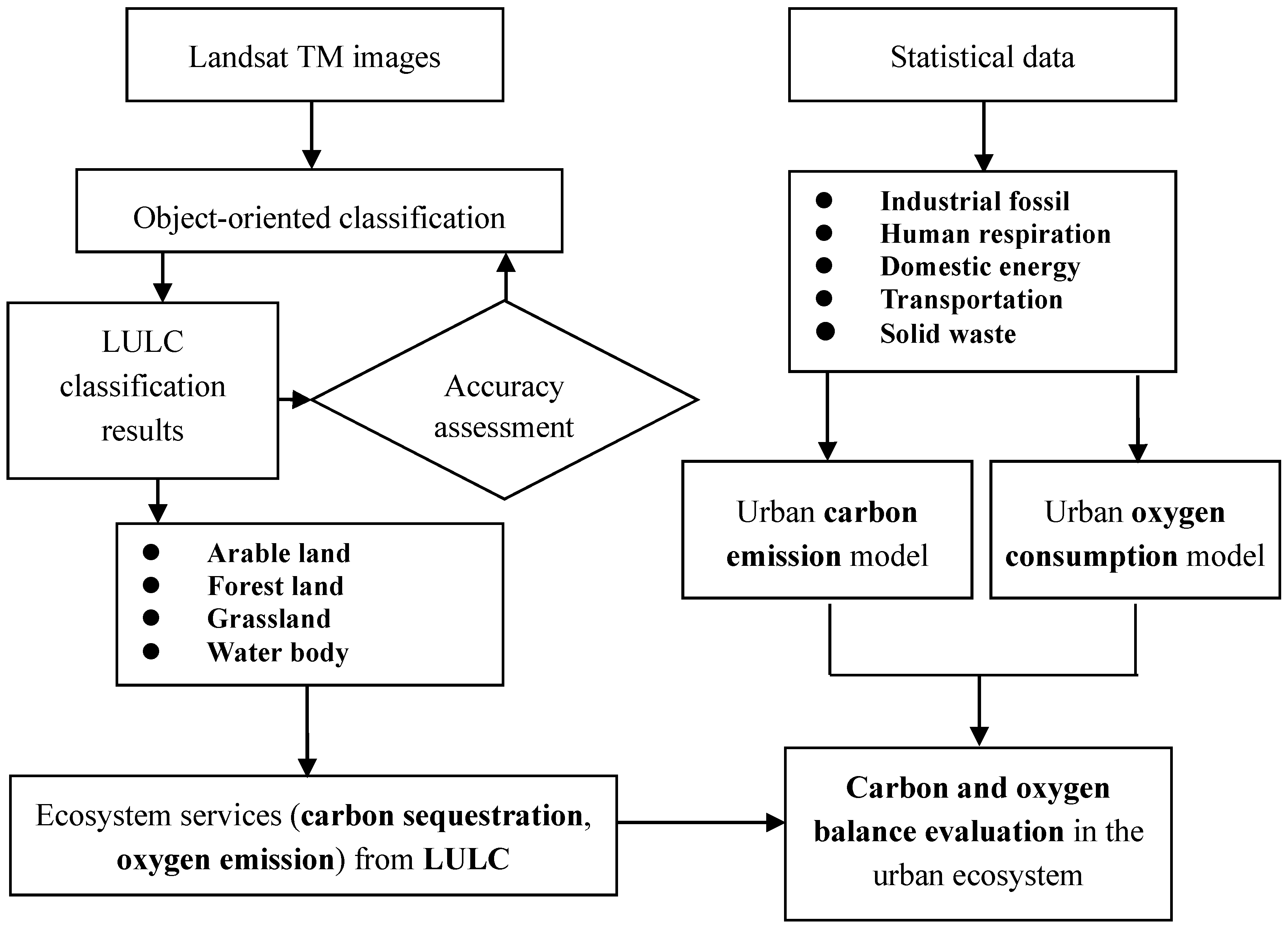
2. Data and Methodology

The methodology to examine the carbon and oxygen balances of the Beijing urban ecosystem (Figure 1) is divided into four main steps: LULC classification, ecosystem services calculation (carbon sequestration and oxygen emissions) from different LULC types, urban carbon emissions and oxygen consumption modeling based on socio-economic statistics, and carbon and oxygen balance evaluations of the urban ecosystem.
First, LULC classification results were generated from Landsat TM images using the object-oriented approach. Second, an urban carbon sequestration model and oxygen emission model were established to calculate the annual ecosystem services calculation (carbon sequestration and oxygen emissions) from different LULC types. Third, an urban carbon emission model and oxygen consumption model were built to calculate the annual carbon emissions and oxygen consumption induced by human activities in an urban area. Finally, relative differences in the carbon and oxygen balances were deduced as assessment indicators to evaluate the carbon and oxygen status of the urban ecosystem.
Figure 1. Research framework.
Sustainability 07 00195 g001

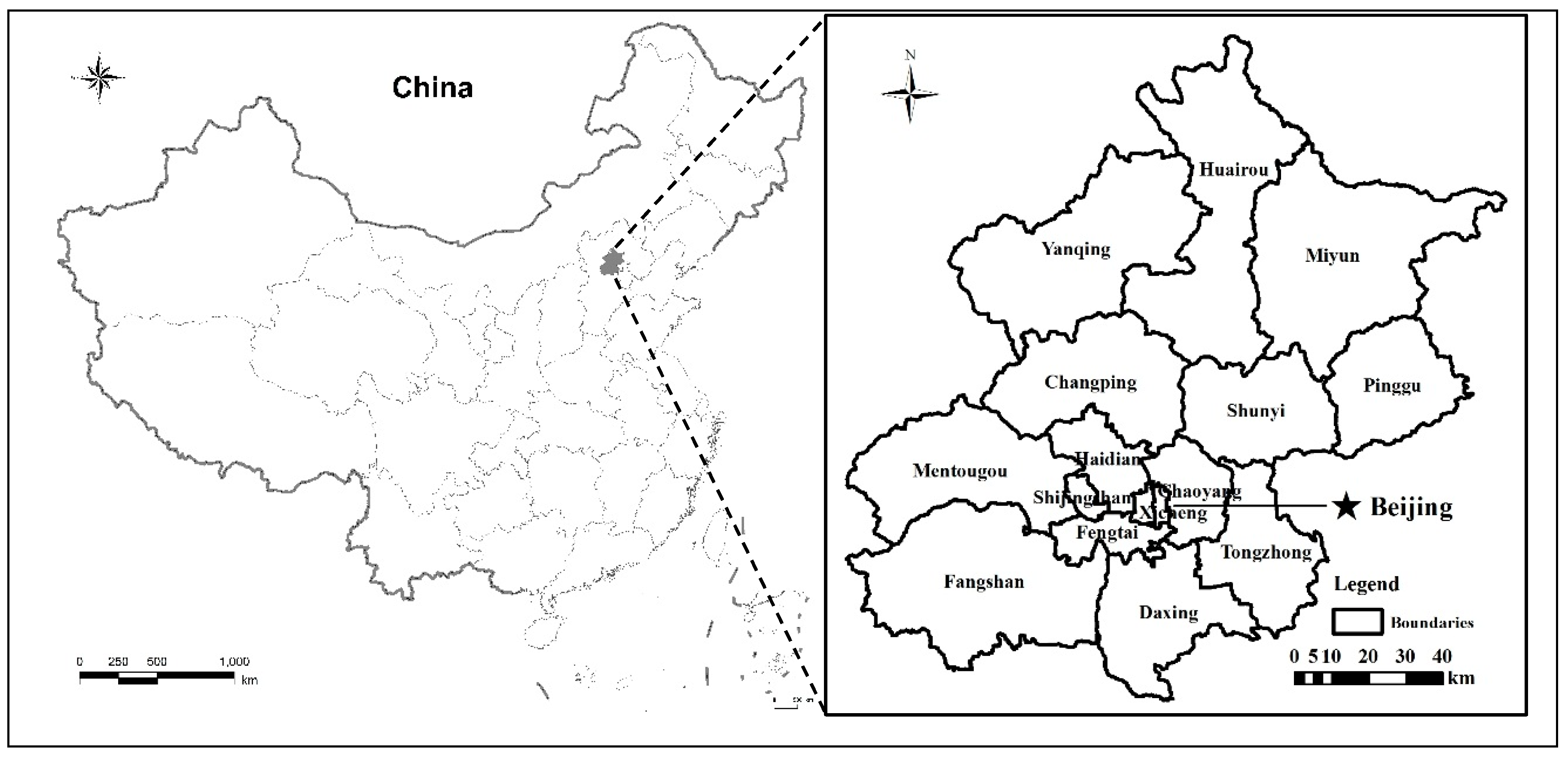
2.1. Study Area and Data Collection

Beijing is located in the North China Plain between the Taihang Mountains and Yanshan Mountains. The mountainous areas account for 62% of the total administrative areas, whereas the plains account for only 38%. The mountainous areas are mainly composed of low terrain. A warm temperate continental monsoon climate with an annual average temperature of 10–12 °C dominates. The annual frost-free period is 180–200 d, and the average annual rainfall is approximately 595 mm. The main land use type is arable land in the plains, whereas deciduous forest and shrub vegetation dominate in the mountains.
The study area covers the entire administrative border of Beijing. Beijing usually refers to the entire area within the administrative borders, including the 16 sub-administrative districts (Figure 2, black lines). High-quality Landsat TM satellite images (path 123/row 32, path 123/row 33 and path 124/row 32) from 2010 (USGS at http://landsat.usgs.gov/index.php) were downloaded to generate the LULC results. The acquisition dates were 08-AUG-2010, 23-JUL-2010 and 15-AUG-2010. The spatial resolution of these TM images is 30 m.
The field sample collection for the LULC classification and calibration was performed from July to September 2010. The total number of samples was 539, of which 50% were used for the LULC classification; the remaining samples used for the accuracy assessment.
The socioeconomic statistics for the urban carbon emissions and oxygen consumption modeling were obtained from the Beijing Statistical Yearbook [90]. The corresponding municipal data included the population, industrial fossil fuel consumption, domestic electricity consumption, transportation fuel consumption, and amount of municipal solid waste. These socioeconomic statistics were all collected at the district scale.
Figure 2. Study area in Beijing, China.
Sustainability 07 00195 g002

2.2. LULC Classification

2.2.1. Object-Oriented Classification

In this study, an object-oriented approach and decision tree were used for the LULC classification. Based on field survey data and our research objectives, the Beijing LULC was classified into six categories: arable land (AL), forest land (FL), grassland (GL), built-up area (BU), water body (WB), and bare land (BL). Initially, the multi-scale image segmentation was completed using eCognition v8.7 software. After the segmentation parameter experiments were performed, a value of 10 was used as the optimal image segmentation scale. Combined with the field samples, the training sample library was established using the sampling tools of eCognition v8.7 software.

2.2.2. Accuracy Assessment

The accuracy analysis was based on the collected field data using ERDAS 9.3 and the confusion error matrix method. The overall accuracy was evaluated by the error matrix and Kappa coefficient, which were calculated with PA (producer’s accuracy) and UA (user’s accuracy) assessments for each land use type.

2.3. Carbon Sequestration and Oxygen Emission Modeling of Urban Ecosystems

2.3.1. Urban Carbon Sequestration Model

An urban carbon sequestration model has been established to calculate the annual net carbon sequestration within a particular area based on LULC data [89], and the parameters used for the model are shown in Table 1. Here, four LULC types (arable land, forest land, grassland, and water body) were considered in the construction of our model, which included the assumptions that the urban atmosphere within the jurisdictional boundaries is a closed system and that urban carbon sequestration and oxygen emissions from LULC within the urban jurisdictional boundaries should offset the effects of urban carbon emissions and oxygen consumption. All the parameters used to calculate the annual carbon sequestration were strictly selected according to the location of the study area. Each healthy ecosystem has a particular degree of self-purification. Ecologically, the atmospheric pollution of the urban ecosystem should be absorbed by its own purification capacity. We also assumed that there was no carbon capacity in the built-up areas; thus, these areas were not considered carbon sinks equivalent to the other ecosystems.
Table 1. Parameters for the urban carbon sequestration and oxygen emission model.
ParametersValueSource
CNPPi from LULC of forest37.05 t/(ha·a)[29]
CERi from LULC of forest6.47 t/(ha·a)[87]
CNPPi from LULC of arable17.97 t/(ha·a)[87]
CERi from LULC of arable3.56 t/(ha·a)[91]
CNPPi from LULC of grass16.32 t/(ha·a)[29]
CERi from LULC of grass5.67 t/(ha·a)[87]
CNPPi from LULC of water0.57 t/(ha·a)[25]
OEi from LULC of forest27.28 t/(ha·a)[29]
OERi from LULC of forest4.71 t/(ha·a)[92]
OEi from LULC of arable11.20 t/(ha·a)[87]
OERi from LULC of arable3.96 t/(ha·a)[92]
OEi from LULC of grass11.84 t/(ha·a)[87]
OERi from LULC of grass4.12 t/(ha·a)[92]
OEi from LULC of water1.51 t/(ha·a)[25]
Note: CNPPi from LULC of forest represents the annual carbon sequestration per unit area from forest land (t/(ha·a)), and CERi from LULC of forest represents the annual carbon emissions from soil respiration per unit area from forest land (t/(ha·a)). CNPPi from LULC of arable represents the annual carbon sequestration per unit area from arable land (t/(ha·a)), and CERi from LULC of arable represents the annual carbon emissions from soil respiration per unit area from arable land (t/(ha·a)). CNPPi from LULC of grass represents the annual carbon sequestration per unit area from grassland (t/(ha·a)), and CERi from LULC of grass represents the annual carbon emissions from soil respiration per unit area from grassland (t/(ha·a)). CNPPi from LULC of water represents the annual carbon sequestration per unit area from water (t/(ha·a)). OEi from LULC of forest represents the annual oxygen emissions per unit area from forest land (t/(ha·a)), and OERi from LULC of forest represents the annual oxygen consumption from soil respiration per unit area from forest land (t/(ha·a)). OEi from LULC of arable represents the annual oxygen emissions per unit area from arable land (t/(ha·a)), and OERi from LULC of arable represents the annual oxygen consumption from soil respiration per unit area from arable land (t/(ha·a)). OEi from LULC of grass represents the annual oxygen emissions per unit area from grassland (t/(ha·a)), and OERi from LULC of grass represents the annual oxygen consumption from soil respiration per unit area from grassland (t/(ha·a)). OEi from LULC of water represents the annual oxygen emissions per unit area from water (t/(ha·a)).
The annual net carbon sequestration can be expressed as follows:
C a r b o n _ s e q = i = 1 n ( C N P P i   C E R i ) × A i
where Carbon_seq represents the annual carbon sequestration in an urban area in tons of carbon per year (t/a). CNPPi represents the annual carbon sequestration per unit area from an LULC of type i, namely, the net primary productivity in a particular area in tons of carbon per ha per year (t/(ha·a)). CERi represents the annual carbon emissions from soil respiration per unit area from an LULC of type i, namely, the carbon emissions from ecosystem respiration in tons of carbon per ha per year (t/(ha·a)). Ai represents the total area of an LULC of type i (ha). When the LULC type is a water body, CERi is equal to zero.

2.3.2. Urban Oxygen Emission Model

The urban oxygen emission model is established to calculate the annual net oxygen emissions in a particular area using the same method of the urban carbon sequestration model. The parameters of oxygen emission model are provided in Table 1.
The annual net oxygen emissions can be expressed as follows:
O x y g e n _ e m i   = i = 1 n ( O E i   O E R i ) × A i
where Oxygen_emi represents the annual net oxygen emissions in an urban area in tons of oxygen per year (t/a). OEi represents the annual oxygen emissions per unit area from a LULC of type i in tons of oxygen per ha per year (t/(ha·a)). OERi represents the annual oxygen consumption from soil respiration per unit area from a LULC of type i, namely, oxygen consumption from ecosystem respiration in tons of oxygen per ha per year (t/(ha·a)). Ai represents the total area of a LULC of type i (ha). When the LULC type is a water body, OERi is equal to zero.

2.4. Carbon Emissions and Oxygen Consumption Modeling of Urban Ecosystems

2.4.1. Urban Carbon Emission Model

An urban carbon emission model was built to calculate the annual urban carbon emissions that are induced by human activities in an urban area. Based on previous research on an urban carbon and oxygen balance model (UCOB) [89], calculations were introduced, such as a method for calculating transportation fuel consumption [71,72,93] and municipal solid waste [94], to improve the accuracy of the results. The carbon sources discussed in this study are human respiration, industrial fossil fuel consumption, transportation fuel consumption, domestic energy use, and municipal solid waste.
The annual carbon emissions in an urban ecosystem are calculated as follows:
Carbon_emi = CHR + CIF + CTF + CDE + CSW
where Carbon_emi represents the annual urban carbon emissions (t/a), and CHR, CIF, CTF, CDE, and CSW are the annual carbon emissions (t/a) from human respiration, industrial fossil fuel consumption, transportation fuel consumption, domestic energy use, and municipal solid waste in urban ecosystem, respectively. The units (t/a) are tons of carbon per year.
In Equation (3), the five factors are calculated as follows:
  • CHR = R_carbon × p × 365 × 10−3
  • CIF = E_industrial × fcoal
  • CTF = Car_number × distance × g× fgasoline × 365 × 10−6
  • CDE = E_domestic × felectricity × fcoal × 10−3
  • CSW = W_solid × RDOC × fDOC,
where R_carbon represents the average carbon emission per person per day (kg/(person·day)), a parameter estimated by sampling a large number of Chinese people; p represents the population of a particular area; E_industrial represents the annual industrial fossil coal consumption, which can be acquired directly from the Beijing Statistical Yearbook [90]; fcoal represents the carbon emission factor (t·C/t), which proved to be accessible and representative of the Chinese coal-based carbon emission factor [81]; Car_number represents the actual number of vehicles in a particular area; distance represents the driving distance of each vehicle per day (km/day), which is assumed to be 40 (the average commute time across all modes is expected to be pertinent because an increase in this variable is likely to lead to an increase in CO2 emissions (longer trips) in an urbanized area [95]; g represents the estimated amount of fuel combusted for each trip, in which the gasoline is combusted in a medium-freight vehicle (0.265 L/km) [93]; fgasoline represents the conversion factor for gasoline to g C (65.8 g·C/L), which is the parameter from the research on carbon emissions modeling at an urban neighborhood scale [93]; E_domestic represents the domestic electricity use; felectricity represents the conversion factor for electricity to standard coal, which is widely used in China; and W_solid represents the municipal solid waste production, which can also be acquired directly from the Beijing Statistical Yearbook [90]. RDOC is the ratio of biodegradable organic carbon to solid waste (the IPCC-recommended value for an East Asian country is 14% [94]); and fDOC is the actual decomposition ratio of the DOC (50% is the IPCC-recommended value [94]). The abovementioned parameters are listed in Table 2.
Table 2. Parameters for the urban carbon emission and oxygen consumption model.
ParametersValueSource
R_carbon0.90 kg/(person·day)[96]
fcoal0.9769[81]
g0.265 L/km[93]
fgasoline65.8 g/L[93]
felectricity0.404 kg standard coal/kWh[89]
RDOC14%[94]
fDOC50%[94]
R_oxygen0.75 kg/(person·day)[96]
R2O/C2.67[89]
Note: R_carbon represents the average carbon emissions per person per day (kg/(person·day)); fcoal represents the carbon emission factor (t·C/t); g represents the estimated amount of fuel combusted for each trip, i.e., gasoline combusted in a medium-freight vehicle (0.265 L/km); fgasoline represents the conversion factor for gasoline to g·C (65.8 g·C/L); felectricity represents the conversion factor for electricity to standard coal; RDOC is the ratio of biodegradable organic carbon to solid waste (the IPCC-recommended value for an East Asian country is 14%); fDOC is the actual decomposition ratio of the DOC (50% is the IPCC-recommended value); R_oxygen represents the average oxygen consumption per person per day (kg/(person·day)); and R2O/C represents the molecular weight ratios for oxygen/carbon based on 1 mol carbon combined with 1 mol O2 when the carbon from energy and waste are completely combusted.

2.4.2. Urban Oxygen Consumption Model

An urban oxygen consumption model was built to calculate the annual urban oxygen consumption that is induced by human behavior in urban areas. The oxygen consumption sources discussed in this study are human respiration, industrial fossil fuel consumption, transportation fuel consumption, domestic energy use, and municipal solid waste.
The primary human-induced oxygen consumption in an urban region can be expressed as follows:
Oxygen_con = OHR + OIF + OTF + ODE + OSW
where Oxygen_con represents the annual urban oxygen consumption (t/a) and OHR, OIF, OTF, ODE, and OSW represent the annual oxygen consumption (t/a) induced by human respiration, industrial fossil fuel consumption, transportation fuel consumption, domestic energy use, and municipal solid waste in urban ecosystems, respectively. The units (t/a) are tons of oxygen per year.
In Equation (4), the above five factors are calculated as follows:
  • OHR = R_oxygen × p × 365 × 10−3
  • OIF = E_industrial × fcoal × R2O/C
  • OTF = Car_number × distance × g × fgasoline × 365 × 10−6 × R2O/C
  • ODE = E_domestic × felectricity × fcoal × 10−3 × R2O/C
  • OSW = W_solid × RDOC × fDOC × R2O/C,
where R_oxygen represents the average oxygen consumption per person per day (kg/(person·day)), and R2O/C represents the molecular weight ratios for oxygen/carbon based on 1 mol carbon combined with 1 mol O2 when the carbon from energy and waste are completely combusted. The related parameters are listed in Table 2.

2.5. Evaluation of the Carbon and Oxygen Balances of Urban Ecosystems

Under the assumption that an urban ecosystem is a completely closed system, we revised the UCOB evaluation system to determine whether the carbon and oxygen conditions are balanced in the urban ecosystem [89]. The relative differences in the carbon and oxygen balances are deduced as assessment indicators:
C a r b o n _ b a l = C a r b o n _ s e q C a r b o n _ e m i C a r b o n _ e m i
O x y g e n _ b a l = O x y g e n _ e m i O x y g e n _ c o n O x y g e n _ c o n
where Carbon_bal and Oxygen_bal represent the relative differences in the carbon and oxygen balances, respectively. A positive value for the relative difference indicates that the carbon and oxygen balances have improved in the urban ecosystem, and higher values indicate better conditions. A negative value for the relative difference indicates that the carbon and oxygen balances have worsened.

3. Results and Discussion

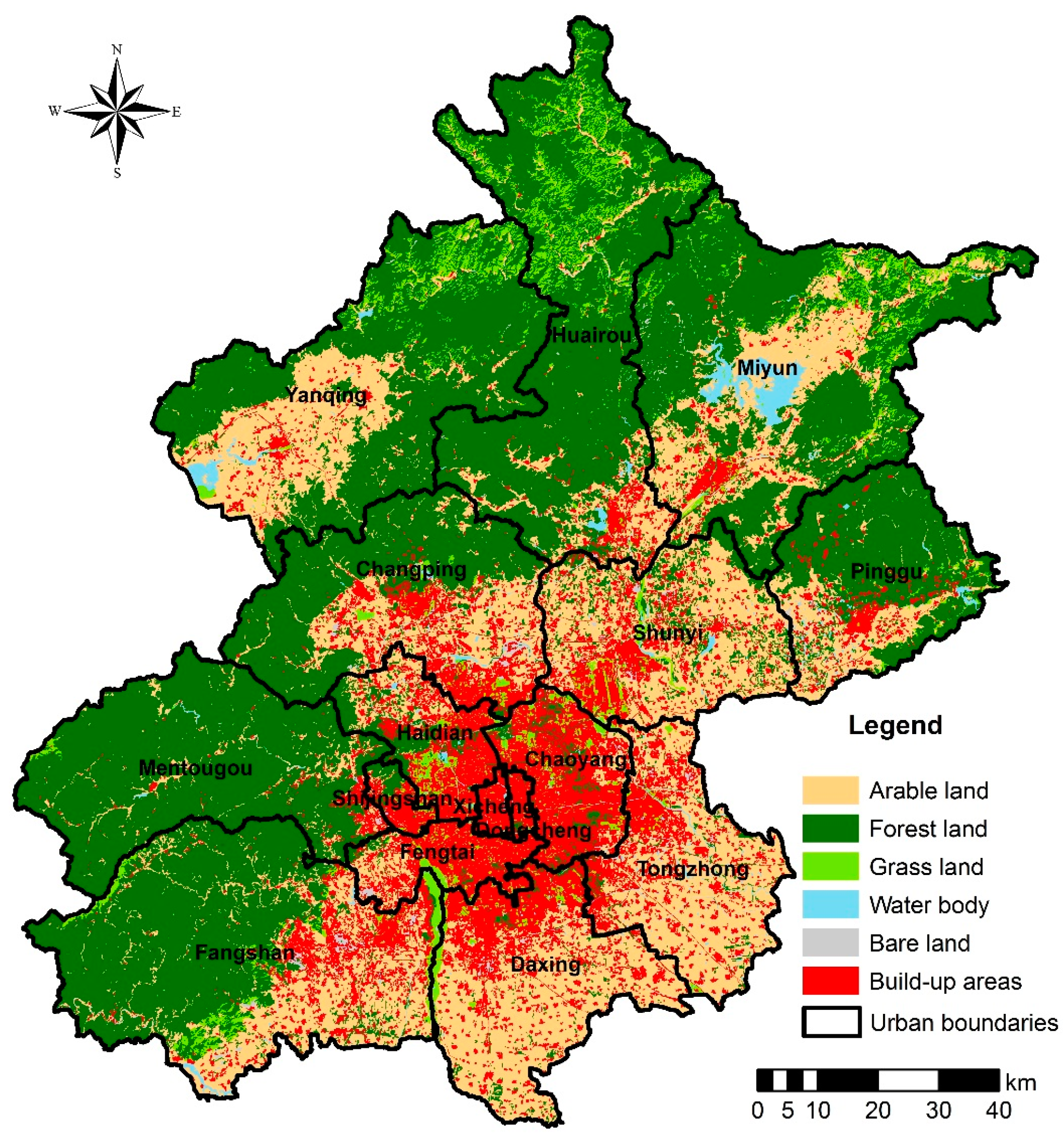
3.1. LULC Classification in Beijing

In this study, a decision tree based on the object-oriented method was used to generate the classification results. The accuracy of each individual LULC class is provided in Table 3, which shows that the overall classification accuracy was 80.89% with a Kappa coefficient of 0.74. Because of the poor resolution of the Landsat images, manual modifications using expert knowledge were required to improve the results of the automatic LULC classification; the results were sufficiently accurate to provide fundamental data sources for carbon sequestration and oxygen emission modeling of urban ecosystems.
Table 3. Accuracy assessment for the LULC results in Beijing.
FLGLWBALBUBL
Area (km2)8468.43867.40267.214128.482589.2071.99
Area (%)51.66%5.29%1.63%25.18%15.79%0.44%
PA90.00%79.31%95.45%44.44%83.54%72.73%
UA74.67%74.19%100.00%72.73%90.73%72.73%
Note: Abbreviations: FL, forest land; GL, grassland; WB, water body; AL, arable land; BU, built-up area; BL, bare land; PA, producer’s accuracy; and UA, user’s accuracy.
The forest and arable lands were the dominant and sub-dominant LULC types, respectively, in Beijing. The area and proportion of the built-up area ranked third (Table 3, Figure 3). Constrained by the mountains to the north and west, the arable land and built-up area were mainly located on the southeast plains. Therefore, the forest land was maintained in the north, northwest, and southwest mountainous areas of Beijing (Figure 3).
Figure 3. Beijing LULC distribution in 2010.
Sustainability 07 00195 g003

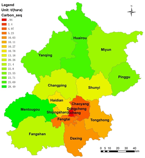
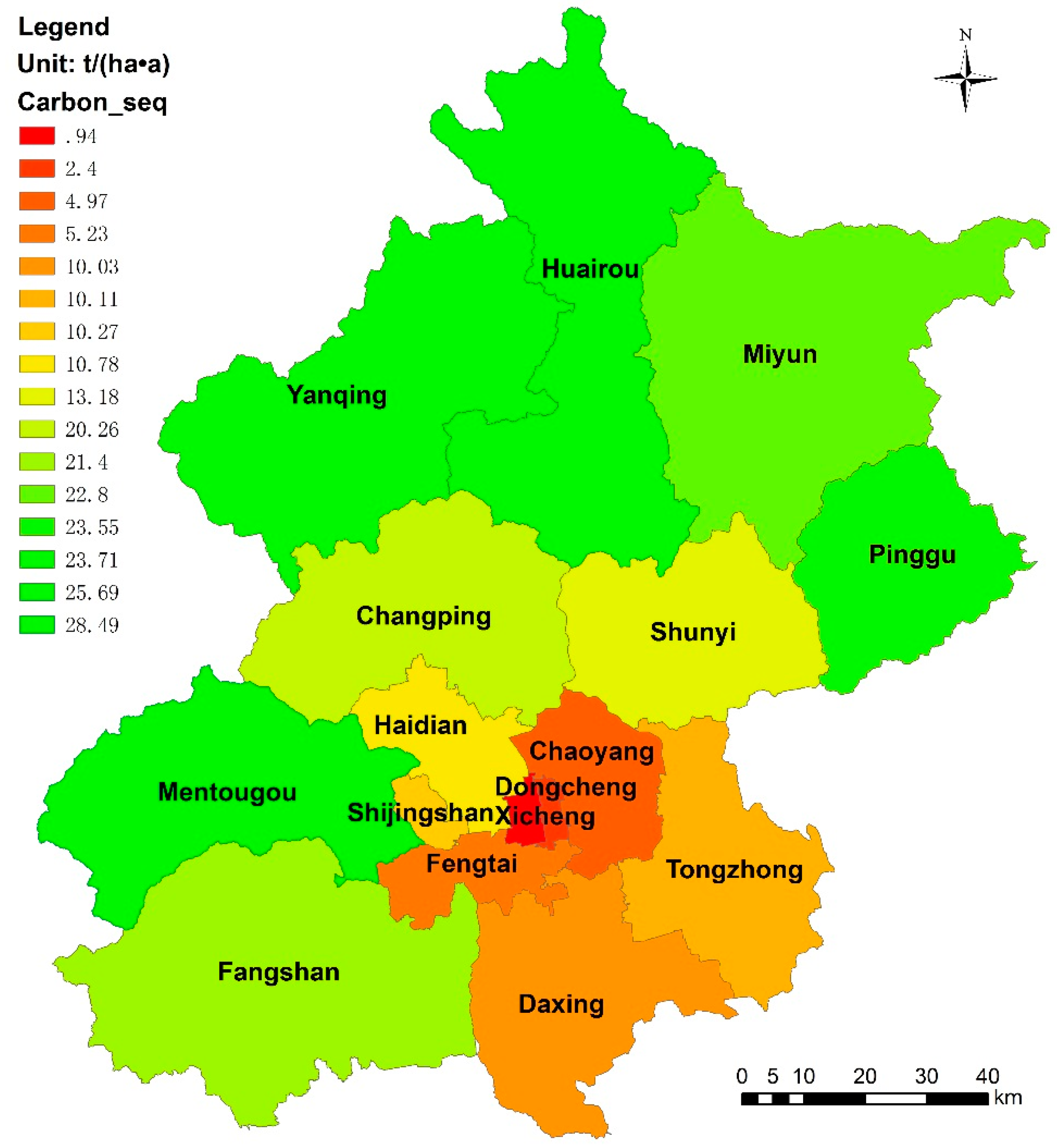
3.2. Spatial Pattern of Carbon Sequestration and Oxygen Emissions from Different LULC Types

The results for the carbon sequestration and oxygen emissions using the proposed models are listed as follows. Table 4 shows the LULC composition of the carbon sinks and oxygen sources. The net carbon sequestration and oxygen emissions in Beijing were 3.28× 10⁷ t/a and 2.28× 10⁷ t/a, respectively. As shown in Table 4, the net carbon sequestration and oxygen emissions were the highest in Huairou compared with all of the districts and counties in Beijing, whereas the values in Xicheng were the lowest.
Table 4. Carbon sequestration and oxygen emissions from different LULC types (Units: t/a).
DistrictsArable LandForest LandGrasslandWater BodyTotal
Carbon sequestrationChangping4.53 × 1052.26 × 1062.98 × 1049.01 × 1022.74 × 106
Chaoyang3.97 × 1041.36 × 1054.97 × 1044.92 × 1022.26 × 105
Daxing8.98 × 1051.12 × 1053.97 × 1043.19 × 1021.05 × 106
Dongcheng 7.21 × 1032.73 × 1035.85 × 1011.00 × 104
Fangshan7.12 × 1053.51 × 1069.83 × 1049.74 × 1024.32 × 106
Fengtai7.22 × 1045.26 × 1043.22 × 1044.63 × 1011.57 × 105
Haidian1.14 × 1053.11 × 1053.82 × 1045.54 × 1024.63 × 105
Huairou2.69 × 1054.94 × 1062.37 × 1057.94 × 1025.45 × 106
Mentougou1.02 × 1053.92 × 1067.88 × 1032.72 × 1024.03 × 106
Miyun7.28 × 1054.16 × 1061.65 × 1055.35 × 1035.06 × 106
Pinggu2.58 × 1051.94 × 1061.97 × 1041.01 × 1032.21 × 106
Shijingshan5.96 × 1037.49 × 1046.52 × 1037.05 × 1018.75 × 104
Shunyi7.73 × 1055.31 × 1054.29 × 1048.72 × 1021.35 × 106
Tongzhong7.92 × 1051.01 × 1051.63 × 1041.69 × 1039.11 × 105
Xicheng 2.43 × 1032.22 × 1039.40 × 1014.74 × 103
Yanqing7.34 × 1053.85 × 1061.30 × 1051.62 × 1034.72 × 106
Beijing5.95 × 1062.59 × 1079.18 × 1051.51 × 1043.28 × 107
Oxygen emissionsChangping2.28 × 1051.67 × 1062.16 × 1042.39 × 1031.92 × 106
Chaoyang1.99 × 1041.00 × 1053.60 × 1041.31 × 1031.58 × 105
Daxing4.51 × 1058.29 × 1042.88 × 1048.44 × 1025.64 × 105
Dongcheng 5.32 × 1031.98 × 1031.55 × 1027.46 × 103
Fangshan3.58 × 1052.59 × 1067.12 × 1042.58 × 1033.02 × 106
Fengtai3.63 × 1043.88 × 1042.33 × 1041.23 × 1029.86 × 104
Haidian5.71 × 1042.30 × 1052.77 × 1041.47 × 1033.16 × 105
Huairou1.35 × 1053.65 × 1061.72 × 1052.10 × 1033.96 × 106
Mentougou5.14 × 1042.89 × 1065.71 × 1037.21 × 1022.95 × 106
Miyun3.66 × 1053.07 × 1061.20 × 1051.42 × 1043.57 × 106
Pinggu1.30 × 1051.43 × 1061.43 × 1042.68 × 1031.58 × 106
Shijingshan3.00 × 1035.53 × 1044.73 × 1031.87 × 1026.32 × 104
Shunyi3.88 × 1053.92 × 1053.11 × 1042.31 × 1038.13 × 105
Tongzhong3.98 × 1057.44 × 1041.18 × 1044.49 × 1034.89 × 105
Xicheng 1.80 × 1031.61 × 1032.49 × 1023.65 × 103
Yanqing3.69 × 1052.84 × 1069.42 × 1044.30 × 1033.31 × 106
Beijing2.99 × 1061.91 × 1076.66 × 1054.01 × 1042.28 × 107
To explain the spatial differences in the carbon sequestration and oxygen emission capacity, the spatial distribution of the carbon sequestration and oxygen emissions per unit area are displayed in Figure 4 and Figure 5, respectively. The carbon density is influenced by the prevailing climate, temperature, illumination time, dominant vegetation, regional development, urbanization level, population density, and land use intensity [2,4,18,19,81,88]. Even a particular type of vegetation at one location may have variable biomass due to the environmental heterogeneity. Therefore, meaningful comparisons across different studies are difficult because of the variation in regions and the methodological approaches used [28,51,93]. Figure 4 and Figure 5 show that the areas with high carbon sequestration and oxygen emissions per unit area were mainly distributed in the exurban counties, such as Mentougou, Huairou, Yanqing, Pinggu, Miyun, and Fangshan. However, the areas with a low capacity for carbon sequestration and oxygen emissions per unit area were mainly distributed in core urban areas that were developed as “downtowns,” such as Xicheng, Dongcheng, and Chaoyang. The carbon sequestration for Hangzhou is 1.66 t/(ha·a) [14], which is between the values for the downtown areas of Xicheng (0.94 t/(ha·a)) and Dongcheng (2.4 t/(ha·a)). In another study, Florence, which has a typical Mediterranean environment, was classified as follows: lawn, forest, mixed vegetation, and lawn with shrubs. The carbon sequestration values were 4.3 t/(ha·a) for lawns and 5.8 t/(ha·a) for forests; mixed vegetation (trees and shrubs) and lawns with shrubs classes were an additional 0.07 t/(ha·a) [17]. The carbon sequestration considerably varied because of the heterogeneous land cover. Our research was subjected to the spatial resolution of the satellite images, so the area cannot be classified into specific categories as was done with Florence.
Figure 4. Distribution of carbon sequestration per unit area in Beijing.
Sustainability 07 00195 g004
Figure 5. Distribution of oxygen emissions per unit area in Beijing.
Sustainability 07 00195 g005
Table 5 shows the carbon sequestration associated with different LULC types in Beijing. We can conclude that the contribution of forest land to carbon sequestration was dominant among the four land use types, particularly in the exurban mountainous regions. The carbon sequestration in Daxing, Tongzhou, and Shunyi was mainly from arable land, and the carbon sequestration from grassland was higher in Xicheng and Dongcheng than in the other districts; thus, grassland is an important carbon sink in downtown areas. The carbon sequestration contribution from water is small compared with the carbon sinks created by forests and arable land. Table 6 shows that the oxygen emission contributions of different LULC types in Beijing exhibited the same pattern as the carbon sequestration for the same LULC types.
Table 5. The percentages of carbon sequestration in different LULC types at the district scale.
DistrictCS-ALCS-FLCS-GLCS-WB
Changping16.52%82.36%1.09%0.03%
Chaoyang17.57%60.21%22.00%0.22%
Daxing85.50%10.69%3.78%0.03%
Dongcheng0.00%72.15%27.27%0.58%
Fangshan16.48%81.22%2.27%0.02%
Fengtai45.97%33.50%20.50%0.03%
Haidian24.51%67.12%8.25%0.12%
Huairou4.94%90.70%4.34%0.01%
Mentougou2.54%97.26%0.20%0.01%
Miyun14.38%82.24%3.27%0.11%
Pinggu11.67%87.40%0.89%0.05%
Shijingshan6.82%85.65%7.45%0.08%
Shunyi57.37%39.38%3.19%0.06%
Tongzhong86.95%11.08%1.79%0.19%
Xicheng0.00%51.30%46.72%1.98%
Yanqing15.55%81.66%2.75%0.03%
Note: The values are the percentages of carbon sequestration in different LULC types. The carbon sequestration contributions of arable land, forest land, grassland, and water bodies are abbreviated CS_AL, CS_FL, CS_GL, and CS_WB, respectively.
Table 6. The percentages of oxygen emissions from different LULC types at the district scale.
DistrictOE-ALOE-FLOE-GLOE-WB
Changping11.86%86.89%1.13%0.12%
Chaoyang12.65%63.67%22.85%0.83%
Daxing80.04%14.71%5.10%0.15%
Dongcheng0.00%71.41%26.51%2.08%
Fangshan11.84%85.72%2.36%0.09%
Fengtai36.80%39.39%23.68%0.12%
Haidian18.07%72.69%8.78%0.47%
Huairou3.42%92.19%4.34%0.05%
Mentougou1.74%98.04%0.19%0.02%
Miyun10.24%86.01%3.36%0.40%
Pinggu8.24%90.68%0.91%0.17%
Shijingshan4.74%87.49%7.48%0.30%
Shunyi47.74%48.15%3.83%0.28%
Tongzhong81.43%15.24%2.42%0.92%
Xicheng0.00%49.18%43.99%6.83%
Yanqing11.13%85.89%2.84%0.13%
Note: The values are the percentages of oxygen emissions from the different LULC types. The oxygen emission contributions of arable land, forest land, grassland, and water bodies are abbreviated OE_AL, OE_FL, OE_GL, and OE_WB, respectively.

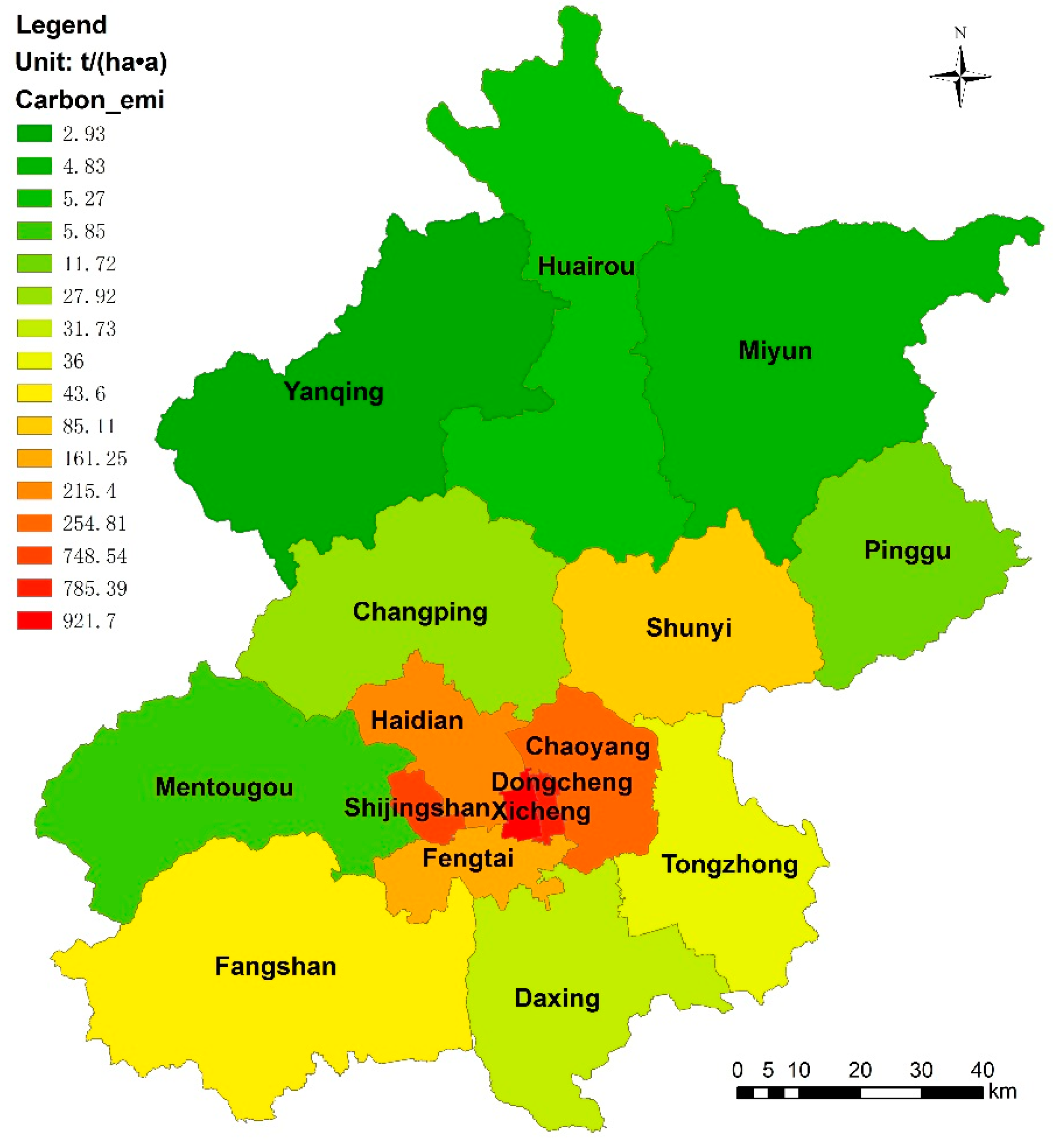
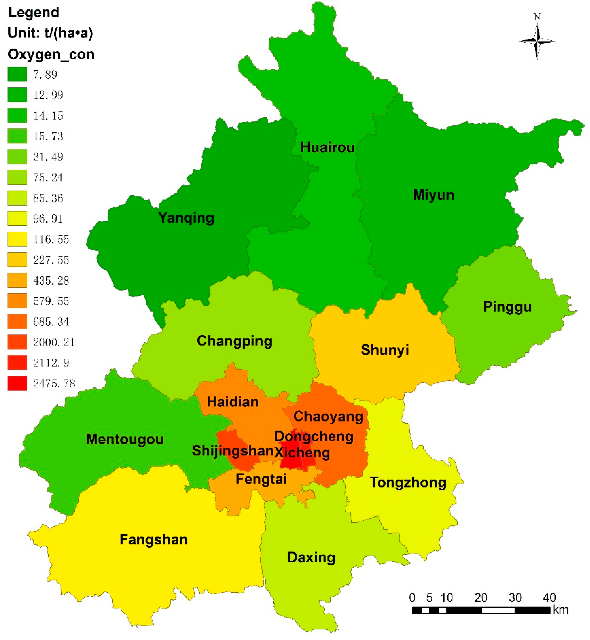
3.3. Estimation of Carbon Emissions and Oxygen Consumption Based on Socioeconomic Statistics

Using the urban carbon emission and oxygen consumption models built in this study, we calculated the human-induced carbon emissions and oxygen consumption of urban ecosystems. The total carbon emissions and oxygen consumption in Beijing were 7.25 × 10⁷ t/a and 1.95 × 10⁸ t/a, respectively (Table 7). The results showed that industrial fossil fuel consumption in the five subsystems contributed to over 75% of the total carbon emissions and oxygen consumption for all 16 districts in Beijing. Most of the carbon emissions originated from urban industrial areas as a result of burning fossil fuels, including coal, oil, and natural gas [5]. Based on the CO2 emission inventories method, which is recommended by the IPCC, Geng and other authors studied the Beijing CO2 emission inventories according to fuel type from 1990 to 2007; the results showed that coal combustion accounted for over 60% of the total CO2 emissions in Beijing over the past two decades, similar to our results. Chuai et al. also reported that carbon emissions from traditional fossil-fuel energy consumption were one of the main causes of global warming [46]. Using the input–output structural decomposition analysis model, production structure change and population growth were the two main drivers for increasing CO2 emissions in Beijing over 1997–2010 [79]. A three-scale input–output model for an urban economy is presented using a case study on CO2 emissions, in which carbon emissions from coal account for 56.81% of the total emissions in Beijing [86]. The research on simulating energy consumption and CO2 emissions at the urban scale in the United States indicated that depending on the definition of urban, between 37% and 86% of direct fuel consumption in buildings and industry and between 37% and 77% of on-road gasoline and diesel consumption occurs in urban areas [97]. The percentages for other human-induced carbon sources, such as domestic energy use, human respiration, transportation, and municipal solid waste, were relatively lower. In addition, the total carbon emissions and oxygen consumption of different regions showed that Chaoyang was the largest carbon source in Beijing and that Yanqing had the lowest value of carbon emissions and oxygen consumption. Landscape fragmentation is highly positively correlated with total CO2 emissions and negatively correlated with CO2 uptake [17].
Table 7. Total human-induced carbon emissions and oxygen consumption in the urban ecosystems (Units: t/a).
DistrictsIndustrial Fossil FuelHuman RespirationDomestic EnergyTransportationSolid WasteTotal
Carbon emissionsChangping3.11 × 1061.49 × 1054.13 × 1057.94 × 1043.15 × 1043.78 × 106
Chaoyang9.77 1063.18 × 1051.18 × 1062.15 × 1059.02 × 1041.16 × 106
Daxing2.84 × 1061.22 × 1052.54 × 1057.37 × 1042.89 × 1043.32 × 106
Dongcheng2.70 × 1068.23 × 1043.76 × 1058.26 × 1043.15 × 1043.28 × 106
Fangshan8.48 × 1068.47 × 1041.84 × 1054.75 × 1041.19 × 1048.81 × 106
Fengtai3.74 × 1061.89 × 1057.04 × 1051.44 × 1056.18 × 1044.84 × 106
Haidian7.82 × 1062.94 × 1058.87 × 1051.89 × 1056.35 × 1049.26 × 106
Huairou9.81 × 1053.34 × 1047.64 × 1041.95 × 1047.67 × 1031.12 × 106
Mentougou7.08 × 1052.60 × 1047.18 × 1041.45 × 1046.95 × 1038.28 × 105
Miyun9.13 × 1054.19 × 1049.15 × 1041.78 × 1047.40 × 1031.07 × 106
Pinggu9.67 × 1053.73 × 1047.43 × 1041.81 × 1045.58 × 1031.10 × 106
Shijingshan6.17 × 1065.52 × 1041.13 × 1053.24 × 1049.28 × 1036.38 × 106
Shunyi8.30 × 1067.86 × 1042.58 × 1054.70 × 1041.20 × 1048.70 × 106
Tongzhong2.72 × 1061.06 × 1053.41 × 1055.65 × 1041.62 × 1043.24 × 106
Xicheng4.02 × 1061.11 × 1053.94 × 1051.03 × 1054.07 × 1044.67 × 106
Yanqing4.88 × 1052.84 × 1044.96 × 1041.21 × 1044.35 × 1035.83 × 105
Beijing6.37 × 1071.76 × 1065.47 × 1061.15 × 1064.30 × 1057.25 × 107
Oxygen consumptionChangping8.28 × 1064.55 × 1051.15 × 1062.12 × 1058.40 × 1041.02 × 107
Chaoyang2.61 × 1079.70 × 1053.28 × 1065.73 × 1052.40 × 1053.11 × 107
Daxing7.58 × 1063.74 × 1057.08 × 1051.97 × 1057.71 × 1048.94 × 106
Dongcheng7.21 × 1062.52 × 1051.05 × 1062.20 × 1058.41 × 1048.81 × 106
Fangshan2.26 × 1072.59 × 1055.14 × 1051.27 × 1053.18 × 1042.35 × 107
Fengtai9.98 × 1065.78 × 1051.96 × 1063.85 × 1051.65 × 1051.31 × 107
Haidian2.09 × 1078.98 × 1052.47 × 1065.05 × 1051.69 × 1052.49 × 107
Huairou2.62 × 1061.02 × 1052.13 × 1055.19 × 1042.05 × 1043.00 × 106
Mentougou1.89 × 1067.94 × 1042.00 × 1053.87 × 1041.85 × 1042.23 × 106
Miyun2.43 × 1061.28 × 1052.55 × 1054.75 × 1041.97 × 1042.88 × 106
Pinggu2.58 × 1061.14 × 1052.07 × 1054.82 × 1041.49 × 1042.96 × 106
Shijingshan1.64 × 1071.69 × 1053.15 × 1058.63 × 1042.48 × 1041.70 × 107
Shunyi2.21 × 1072.40 × 1057.19 × 1051.25 × 1053.21 × 1042.33 × 107
Tongzhong7.26 × 1063.24 × 1059.50 × 1051.51 × 1054.33 × 1048.73 × 106
Xicheng1.07 × 1073.40 × 1051.10 × 1062.75 × 1051.08 × 1051.26 × 107
Yanqing1.30 × 1068.68 × 1041.38 × 1053.22 × 1041.16 × 1041.57 × 106
Beijing1.70 × 1085.37 × 1061.50 × 1073.07 × 1061.15 × 1061.95 × 108
Figure 6 and Figure 7 show the spatial distribution of carbon emissions and oxygen consumption per unit area. Because of the lower levels of economic development and population density, the exurban counties had relatively lower values of carbon emissions and oxygen consumption than the urban and suburban districts. The areas with high values of carbon emissions and oxygen consumption per unit area were mainly concentrated in downtown areas, including Xicheng, Dongcheng, Chaoyang, Haidian, Shijingshan, and Fengtai. According to the eddy covariance CO2 flux measurements for North Beijing over 2008, the annual CO2 emissions from the study site were estimated at 20.6 kg/(m2·a) [66] or 206 t/(ha·a), which was consistent with the yearly emissions of 215.4 t/(ha·a) for Haidian in our results. The annual modeled local emissions in Vancouver, British Columbia, Canada were estimated at 7.42 kg/(m2·a) with direct eddy covariance measurements. This value equals 74.2 t/(ha·a), which is much lower than the value of 215.4 t/(ha·a) for Haidian in our results [68]. The annual carbon emission value of 74.2 t/(ha·a) in Vancouver is close to the value of 85.11 t/(ha·a) in Shunyi, which indicates similar urbanization levels in these two areas.

3.4. Data Limitation and Uncertainty Analysis

While uncertainties in the carbon budget itself are mainly assigned to data and system definitions, the methodology for assessing the impact of reduction measures includes different types of uncertainty [10].
The overall LULC classification accuracy of the study area was 80.89%, which met the demand of the research. Because of the lower resolution of TM images, the LULC was classified into six broad categories: arable land, forest land, grassland, built-up area, water body, and bare land. The LULC classification cannot attain the secondary classification level, such as evergreen coniferous forest or broadleaved deciduous forest. Moreover, the field data corresponding to the LULC classification of the secondary classes were scarce. In reality, many of the built-up areas in large cities such as Beijing are vegetated and have varying amounts of plant cover. However, we did not consider the pixels and patches of these small green spaces in the built-up landscape of Beijing because of the resolution of the TM images. All of these factors affect the final calculation accuracy of the carbon sequestration and oxygen emissions. Therefore, the actual carbon sink for the study area may have been underestimated.
Figure 6. Distribution of carbon emissions per unit area in Beijing.
Sustainability 07 00195 g006
Figure 7. Distribution of oxygen consumption per unit area in Beijing.
Sustainability 07 00195 g007
Commonly, numerous parameters and factors that are used to build ecosystem models are highly uncertain. Because CO2 emission data for all carbon sources in Beijing are not currently provided at the district scale, acquiring all the data officially is difficult. For example, there is an absence of statistical data on livestock in the districts. The results of human-induced carbon emissions and oxygen consumption were slightly lower than the real values without considering the livestock respiration. In addition, the transportation carbon emissions must be calculated based on the actual regional fuel consumption, rather than the number of vehicles. The carbon emission results for municipal solid waste can be also improved using more exact experimental parameters.
Thus, to improve the model’s accuracy, further efforts are needed to obtain high-resolution LULC results and field experiment data in the future.

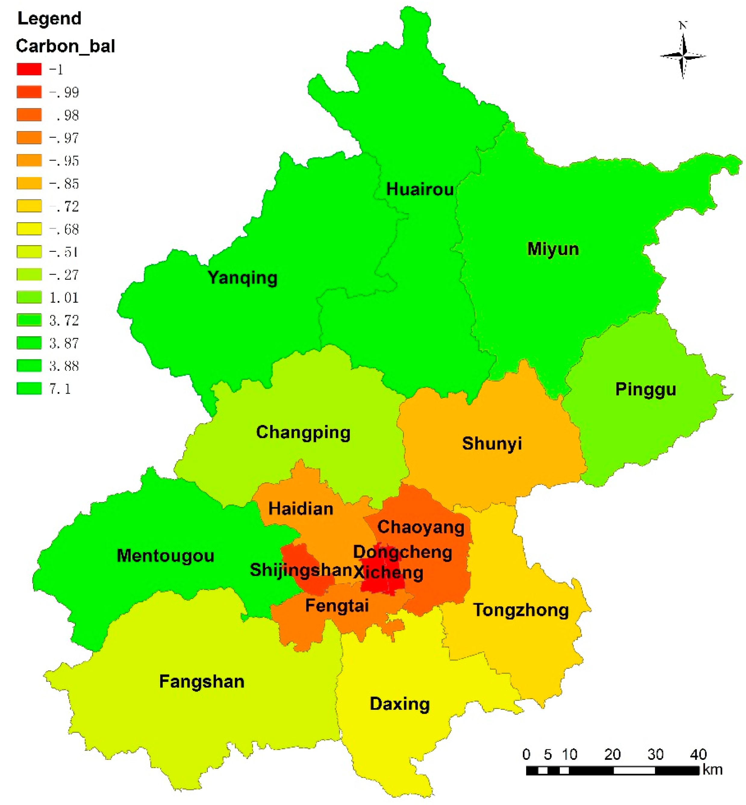
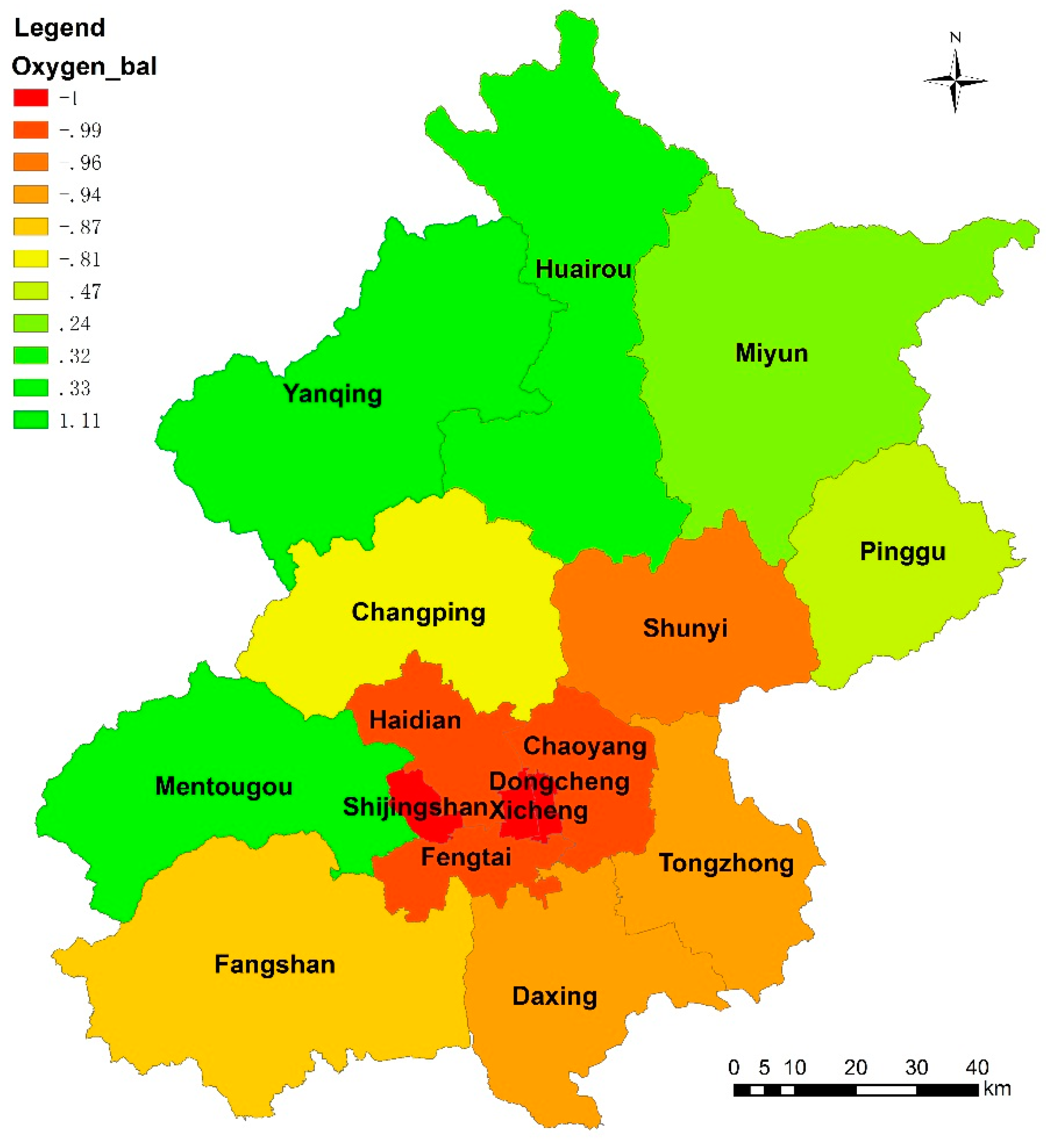
3.5. Evaluation of the Carbon and Oxygen Balances in Urban Ecosystems

Based on the detailed models, the Carbon_bal and Oxygen_bal relative differences for the entirety of the Beijing area and its sub-administrative areas were calculated to evaluate the carbon and oxygen balances of an urban ecosystem (Table 8). The results showed that the carbon sequestration and oxygen emissions within Beijing cannot meet the demand for urban carbon emissions and oxygen consumption. The relative differences of Carbon_bal and Oxygen_bal in Yanqing, Huairou, Mentougou, and Miyun were all positive, which indicated that the carbon and oxygen balances in these urban ecosystems were superior; however, all four of these counties are located in exurban regions (Figure 8 and Figure 9).
Table 8. Carbon and oxygen balance relative differences of the urban ecosystem.
DistrictsCarbon_balOxygen_bal
Changping−0.2742−0.8116
Chaoyang−0.9805−0.9949
Daxing−0.6838−0.9369
Dongcheng−0.9969−0.9992
Fangshan−0.5091−0.8716
Fengtai−0.9676−0.9925
Haidian−0.9499−0.9873
Huairou3.87640.3180
Mentougou3.87070.3261
Miyun3.72300.2382
Pinggu1.0099−0.4681
Shijingshan−0.9863−0.9963
Shunyi−0.8451−0.9650
Tongzhong−0.7191−0.9440
Xicheng−0.9990−0.9997
Yanqing7.09701.1076
Beijing−0.5479−0.8828
Figure 8. Carbon balances in the districts of Beijing.
Sustainability 07 00195 g008
Figure 9. Oxygen balances in the districts of Beijing.
Sustainability 07 00195 g009
Compared with the exurban districts that showed good carbon and oxygen balances, the districts whose Carbon_bal and Oxygen_bal relative differences were negative were almost all located in the core areas of the urban and suburban districts (Figure 8 and Figure 9). These core areas of the urban and suburban areas worsened the carbon and oxygen balances. Thus, measures to improve the carbon and oxygen balances in these areas are urgently needed [98].

4. Conclusions

Based on the LULC data and empirical coefficients, the carbon sequestration and oxygen emission model can produce reasonable estimates of urban ecosystem services that sequester carbon and emit oxygen. The areas with a high capacity for carbon sequestration and oxygen emissions were mainly distributed in the exurban districts of Beijing, whereas the areas with a poor capacity were mainly distributed in the core urban areas.
Based on the urban carbon emission and oxygen consumption model built in this study, the sources of human-induced carbon emissions and oxygen consumption can be partitioned within the urban ecosystem. The results show that in the five subsystems, the consumption of industrial fossil fuel produced the highest total carbon emissions and oxygen consumption. The contributions from other human-induced carbon sources, such as domestic energy use, human respiration, transportation, and municipal solid waste, were small compared with that of industrial fossil fuel consumption.
The relative differences in the carbon and oxygen balances varied among the 16 districts in Beijing. The carbon and oxygen balances in the exurban districts were improved over those of the core urban areas. Variations in the different regions were a result of the level of urbanization, LULC distribution, economic structure, population, and fossil energy consumption. As shown in this study, forest, arable land, grassland, and water can play important roles in offsetting urban carbon emissions; thus, urban planning and management could be a method of mitigating climate change. Evaluating carbon and oxygen balances in urban ecosystems significantly reduces the burden on urban planners and government policymakers to understand current emissions. The methods developed in this research are viable for the quantitative evaluation of urban ecosystem carbon and oxygen balances.

Acknowledgments

This research is supported by the Natural Science Foundation of China (no. 41101501, no. 41471423 and no. 41371540), and China High-Resolution Earth Observation System (CHEOS) (no. 01-Y30B16-9001-14/16-02). The comments from the anonymous reviewers helped to substantially improve the manuscript.

Author Contributions

Kai Yin and Yichen Tian mainly contributed to the design, data collection, and analysis. Kai Yin and Dengsheng Lu participated in drafting the article. Kai Yin and Qianjun Zhao were responsible for revising the article. Chao Yuan was responsible for data processing. All of the authors read and approved the final version of the manuscript.

Conflicts of Interest

The authors declare no conflicts of interest.

References

  1. Lenzen, M.; Pade, L.L.; Munksgaard, J. CO2 multipliers in multi-region input-output models. Econ. Syst. Res. 2004, 16, 391–412. [Google Scholar] [CrossRef]
  2. Churkina, G.; Brown, D.G.; Keoleian, G. Carbon stored in human settlements: The conterminous united states. Glob. Chang. Biol. 2010, 16, 135–143. [Google Scholar] [CrossRef]
  3. Sullivan, P. Energetic cities energy, environment and strategic thinking. World Policy J. 2010, 27, 11–13. [Google Scholar] [CrossRef]
  4. Hutyra, L.R.; Yoon, B.; Alberti, M. Terrestrial carbon stocks across a gradient of urbanization: A study of the seattle, wa region. Glob. Chang. Biol. 2011, 17, 783–797. [Google Scholar] [CrossRef]
  5. Churkina, G. Modeling the carbon cycle of urban systems. Ecol. Model. 2008, 216, 107–113. [Google Scholar] [CrossRef]
  6. Zhu, X.-J.; Yu, G.R.; He, H.L.; Wang, Q.F.; Chen, Z.; Gao, Y.N.; Zhang, Y.P.; Zhang, J.H.; Yan, J.H.; Wang, H.M.; et al. Geographical statistical assessments of carbon fluxes in terrestrial ecosystems of china: Results from upscaling network observations. Glob. Planet. Chang. 2014, 118, 52–61. [Google Scholar] [CrossRef]
  7. Song, C.; Woodcock, C.E. A regional forest ecosystem carbon budget model: Impacts of forest age structure and landuse history. Ecol. Model. 2003, 164, 33–47. [Google Scholar] [CrossRef]
  8. Wang, S.; Fang, C.; Wang, Y.; Huang, Y.; Ma, H. Quantifying the relationship between urban development intensity and carbon dioxide emissions using a panel data analysis. Ecol. Indic. 2015, 49, 121–131. [Google Scholar] [CrossRef]
  9. Feng, K.; Hubacek, K.; Sun, L.; Liu, Z. Consumption-based CO2 accounting of china’s megacities: The case of beijing, tianjin, shanghai and chongqing. Ecol. Indic. 2014, 47, 26–31. [Google Scholar] [CrossRef]
  10. Walz, A.; Calonder, G.P.; Hagedorn, F.; Lardelli, C.; Lundström, C.; Stöckli, V. Regional CO2 budget, countermeasures and reduction aims for the alpine tourist region of davos, switzerland. Energy Policy 2008, 36, 811–820. [Google Scholar] [CrossRef]
  11. Hayha, T.; Franzese, P.P. Ecosystem services assessment: A review under an ecological-economic and systems perspective. Ecol. Model. 2014, 289, 124–132. [Google Scholar] [CrossRef]
  12. De Groot, R.S.; Alkemade, R.; Braat, L.; Hein, L.; Willemen, L. Challenges in integrating the concept of ecosystem services and values in landscape planning, management and decision making. Ecol. Complex. 2010, 7, 260–272. [Google Scholar]
  13. Cox, P.M.; Betts, R.A.; Jones, C.D.; Spall, S.A.; Totterdell, I.J. Acceleration of global warming due to carbon-cycle feedbacks in a coupled climate model. Nature 2000, 408, 184–187. [Google Scholar] [CrossRef] [PubMed]
  14. Zhao, M.; Kong, Z.-H.; Escobedo, F.J.; Gao, J. Impacts of urban forests on offsetting carbon emissions from industrial energy use in hangzhou, china. J. Environ. Manag. 2010, 91, 807–813. [Google Scholar] [CrossRef]
  15. Weissert, L.; Salmond, J.; Schwendenmann, L. A review of the current progress in quantifying the potential of urban forests to mitigate urban CO2 emissions. Urban Clim. 2014, 8, 100–125. [Google Scholar] [CrossRef]
  16. Lin, W.; Wu, T.; Zhang, C.; Yu, T. Carbon savings resulting from the cooling effect of green areas: A case study in beijing. Environ. Pollut. 2011, 159, 2148–2154. [Google Scholar] [CrossRef] [PubMed]
  17. Vaccari, F.P.; Gioli, B.; Toscano, P.; Perrone, C. Carbon dioxide balance assessment of the city of florence (italy), and implications for urban planning. Landsc. Urban Plan. 2013, 120, 138–146. [Google Scholar] [CrossRef]
  18. Lloyd, J.; Shibistova, O.; Zolotoukhine, D.; Kolle, O.; Arneth, A.; Wirth, C.; Styles, J.M.; Tchebakova, N.M.; Schulze, E.D. Seasonal and annual variations in the photosynthetic productivity and carbon balance of a central siberian pine forest. Tellus Ser. B 2002, 54, 590–610. [Google Scholar] [CrossRef]
  19. Kolari, P.; Pumpanen, J.; Rannik, U.; Ilvesniemi, H.; Hari, P.; Berninger, F. Carbon balance of different aged scots pine forests in southern finland. Glob. Chang. Biol. 2004, 10, 1106–1119. [Google Scholar] [CrossRef]
  20. McGuire, A.; Sitch, S.; Clein, J.; Dargaville, R.; Esser, G.; Foley, J.; Heimann, M.; Joos, F.; Kaplan, J.; Kicklighter, D. Carbon balance of the terrestrial biosphere in the twentieth century: Analyses of co2, climate and land use effects with four process—Based ecosystem models. Glob. Biogeochem. Cycles 2001, 15, 183–206. [Google Scholar] [CrossRef]
  21. Kelsey, K.; Neff, J. Estimates of aboveground biomass from texture analysis of landsat imagery. Remote Sens. 2014, 6, 6407–6422. [Google Scholar] [CrossRef]
  22. Lestan, K.; Eržen, I.; Golobič, M. The role of open space in urban neighbourhoods for health-related lifestyle. Int. J. Environ. Res. Public Health 2014, 11, 6547–6570. [Google Scholar] [CrossRef] [PubMed]
  23. Zhao, T.; Brown, D.G.; Fang, H.; Theobald, D.M.; Liu, T.; Zhang, T. Vegetation productivity consequences of human settlement growth in the eastern united states. Landsc. Ecol. 2012, 27, 1149–1165. [Google Scholar] [CrossRef]
  24. Silaydin Aydin, M.B.; Çukur, D. Maintaining the carbon–oxygen balance in residential areas: A method proposal for land use planning. Urban For. Urban Green. 2012, 11, 87–94. [Google Scholar]
  25. Duan, X.N.; Wang, X.K.; Lu, F.; Ouyang, Z.Y. Carbon sequestration and its potential by wetland ecosystems in china. Acta Ecol. Sin. 2008, 28, 463–469. [Google Scholar] [CrossRef]
  26. Dang, Y.; Li, Y.; Sun, R.; Hu, B.; Zhang, T.; Liu, Y. Estimation of Carbon Dioxide Emission in Beijing City. In Proceedings of the Urban Remote Sensing Event, 2009 Joint, Shanghai, China, 20–22 May 2009; pp. 1–6.
  27. Fang, J.; Guo, Z.; Piao, S.; Chen, A. Terrestrial vegetation carbon sinks in china, 1981–2000. Sci. China Ser. D 2007, 50, 1341–1350. [Google Scholar] [CrossRef]
  28. Grimm, N.B.; Faeth, S.H.; Golubiewski, N.E.; Redman, C.L.; Wu, J.; Bai, X.; Briggs, J.M. Global change and the ecology of cities. Science 2008, 319, 756–760. [Google Scholar] [CrossRef] [PubMed]
  29. Jingyun, F.; Guohua, L.; Songling, X. Biomass and net production of forest vegetation in china. Acta Ecol. Sin. 1996, 5, 497–508. [Google Scholar]
  30. Lal, R. Soil carbon sequestration in china through agricultural intensification, and restoration of degraded and desertified ecosystems. Land Degrad. Dev. 2002, 13, 469–478. [Google Scholar] [CrossRef]
  31. Xia, J.; Liu, S.; Liang, S.; Chen, Y.; Xu, W.; Yuan, W. Spatio-temporal patterns and climate variables controlling of biomass carbon stock of global grassland ecosystems from 1982 to 2006. Remote Sens. 2014, 6, 1783–1802. [Google Scholar] [CrossRef]
  32. Pan, G.; Li, L.; Wu, L.; Zhang, X. Storage and sequestration potential of topsoil organic carbon in china's paddy soils. Glob. Chang. Biol. 2004, 10, 79–92. [Google Scholar] [CrossRef]
  33. Wang, S.-X.; Yao, Y.; Zhou, Y. Analysis of ecological quality of the environment and influencing factors in china during 2005–2010. Int. J. Environ. Res. Public Health 2014, 11, 1673–1693. [Google Scholar] [CrossRef] [PubMed]
  34. Maselli, F.; Chiesi, M.; Moriondo, M.; Fibbi, L.; Bindi, M.; Running, S.W. Modelling the forest carbon budget of a mediterranean region through the integration of ground and satellite data. Ecol. Model. 2009, 220, 330–342. [Google Scholar] [CrossRef]
  35. Ito, A. The regional carbon budget of east asia simulated with a terrestrial ecosystem model and validated using asiaflux data. Agric. For. Meteorol. 2008, 148, 738–747. [Google Scholar] [CrossRef]
  36. Chen, Y.; Li, X.; Liu, X.; Ai, B. Analyzing land-cover change and corresponding impacts on carbon budget in a fast developing sub-tropical region by integrating modis and landsat tm/etm+ images. Appl. Geogr. 2013, 45, 10–21. [Google Scholar] [CrossRef]
  37. Trischler, J.; Sandberg, D.; Thörnqvist, T. An approach to estimate the productivity of various species on sites in sweden by choosing individual climate and productivity values and the MIAMI-model with modifications. In Proceedings of the “Climate change and forestry in northern Europe” Workshop, Uppsala, Sweden, 11–12 November 2013; pp. 1–12.
  38. Wang, W.; Dungan, J.; Hashimoto, H.; Michaelis, A.R.; Milesi, C.; Ichii, K.; Nemani, R.R. Diagnosing and assessing uncertainties of terrestrial ecosystem models in a multimodel ensemble experiment: 1. Primary production. Glob. Chang. Biol. 2011, 17, 1350–1366. [Google Scholar] [CrossRef]
  39. Wang, F.; Mladenoff, D.J.; Forrester, J.A.; Keough, C.; Parton, W.J. Global sensitivity analysis of a modified century model for simulating impacts of harvesting fine woody biomass for bioenergy. Ecol. Model. 2013, 259, 16–23. [Google Scholar] [CrossRef]
  40. Mao, D.; Wang, Z.; Wu, C.; Song, K.; Ren, C. Examining forest net primary productivity dynamics and driving forces in northeastern china during 1982–2010. Chin. Geogr. Sci. 2014, 24, 1–16. [Google Scholar] [CrossRef]
  41. Chen, H.; Chen, G.Q.; Ji, X. Cosmic emergy based ecological systems modelling. Commun. Nonlinear Sci. Numer. Simul. 2010, 15, 2672–2700. [Google Scholar] [CrossRef]
  42. Ji, X. Ecological accounting and evaluation of urban economy: Taking beijing city as the case. Commun. Nonlinear Sci. Numer. Simul. 2011, 16, 1650–1669. [Google Scholar] [CrossRef]
  43. Jiang, M.M.; Zhou, J.B.; Chen, B.; Yang, Z.F.; Ji, X.; Zhang, L.; Chen, G.Q. Ecological evaluation of beijing economy based on emergy indices. Commun. Nonlinear Sci. Numer. Simul. 2009, 14, 2482–2494. [Google Scholar] [CrossRef]
  44. Zhang, Y.; Zhao, Y.W.; Yang, Z.F.; Chen, B.; Chen, G.Q. Measurement and evaluation of the metabolic capacity of an urban ecosystem. Commun. Nonlinear Sci. Numer. Simul. 2009, 14, 1758–1765. [Google Scholar] [CrossRef]
  45. Chen, Z.M.; Chen, B.; Chen, G.Q. Cosmic exergy based ecological assessment for a wetland in beijing. Ecol. Model. 2011, 222, 322–329. [Google Scholar] [CrossRef]
  46. Chuai, X.W.; Lai, L.; Huang, X.J.; Zhao, R.Q.; Wang, W.J.; Chen, Z.G. Temporospatial changes of carbon footprint based on energy consumption in china. J. Geogr. Sci. 2012, 22, 110–124. [Google Scholar] [CrossRef]
  47. Wiedmann, T.; Minx, J. A definition of “carbon footprint”. Ecol. Econ. Res. Trends 2007, 2, 55–65. [Google Scholar]
  48. Zhao, R.Q.; Huang, X.J.; Zhong, T.Y.; Peng, J.W. Carbon footprint of different industrial spaces based on energy consumption in china. J. Geogr. Sci. 2011, 21, 285–300. [Google Scholar] [CrossRef]
  49. Yu, G.; Wang, Q.; Liu, Y.; Liu, Y. Conceptual framework of carbon sequestration rate and potential increment of carbon sink of regional terrestrial ecosystem and scientific basis for quantitative carbon authentification. Prog. Geogr. 2011, 30, 771–787. [Google Scholar]
  50. Kok, R.; Benders, R.M.; Moll, H.C. Measuring the environmental load of household consumption using some methods based on input–output energy analysis: A comparison of methods and a discussion of results. Energy Policy 2006, 34, 2744–2761. [Google Scholar] [CrossRef]
  51. Mühle, S.; Balsam, I.; Cheeseman, C. Comparison of carbon emissions associated with municipal solid waste management in germany and the uk. Resour. Conserv. Recycl. 2010, 54, 793–801. [Google Scholar] [CrossRef]
  52. Geng, Y.; Peng, C.; Tian, M. Energy use and CO2 emission inventories in the four municipalities of china. Energy Proced. 2011, 5, 370–376. [Google Scholar] [CrossRef]
  53. Chen, W.; Huang, L.; Xiang, X.; Chen, J.; Sun, L. Gis based ccs source-sink matching models and decision support system. Energy Proced. 2011, 4, 5999–6006. [Google Scholar] [CrossRef]
  54. Yang, J.; Guo, J.; Ma, S. Low-carbon city logistics distribution network design with resource deployment. J. Clean. Prod. 2013, 85, 453–461. [Google Scholar]
  55. Zhang, Y.; Zheng, H.; Fath, B.D. Analysis of the energy metabolism of urban socioeconomic sectors and the associated carbon footprints: Model development and a case study for beijing. Energy Policy 2014, 73, 540–551. [Google Scholar] [CrossRef]
  56. Qi, Y.; Xie, G.; Ge, L.; Zhang, C.; Li, S. Estimation of china’s carbon footprint based on apparent consumption. Resour. Sci. 2010, 32, 2053–2058. [Google Scholar]
  57. Li, L.; Chen, C.; Xie, S.; Huang, C.; Cheng, Z.; Wang, H.; Wang, Y.; Huang, H.; Lu, J.; Dhakal, S. Energy demand and carbon emissions under different development scenarios for shanghai, China. Energy Policy 2010, 38, 4797–4807. [Google Scholar] [CrossRef]
  58. Xie, H.; Chen, X.; Lin, K.; Hu, A. The ecological footprint analysis of fossil energy and electricity. Acta Ecol. Sin. 2008, 28, 1729–1735. [Google Scholar]
  59. Hubacek, K.; Sun, L. A scenario analysis of china's land use and land cover change: Incorporating biophysical information into input–output modeling. Struct. Chang. Econ. Dyn. 2001, 12, 367–397. [Google Scholar] [CrossRef]
  60. Chen, B.; Chen, G.Q. Ecological footprint accounting based on emergy—A case study of the chinese society. Ecol. Model. 2006, 198, 101–114. [Google Scholar] [CrossRef]
  61. Shao, L.; Wu, Z.; Chen, G.Q. Exergy based ecological footprint accounting for china. Ecol. Model. 2013, 252, 83–96. [Google Scholar] [CrossRef]
  62. Chen, B.; Chen, G.Q.; Yang, Z.F.; Jiangc, M.M. Ecological footprint accounting for energy and resource in china. Energy Policy 2007, 35, 1599–1609. [Google Scholar] [CrossRef]
  63. Chen, B.; Chen, G.Q. Modified ecological footprint accounting and analysis based on embodied exergy—A case study of the chinese society 1981–2001. Ecol. Econ. 2007, 61, 355–376. [Google Scholar] [CrossRef]
  64. Dong, Y.; Xia, B.; Chen, W. Carbon footprint of urban areas: An analysis based on emission sources account model. Environ. Sci. Policy 2014, 44, 181–189. [Google Scholar] [CrossRef]
  65. Song, T.; Wang, Y.; Sun, Y. Estimation of carbon dioxide flux and source partitioning over beijing, china. J. Environ. Sci. 2013, 25, 2429–2434. [Google Scholar] [CrossRef]
  66. Song, T.; Wang, Y. Carbon dioxide fluxes from an urban area in beijing. Atmos. Res. 2012, 106, 139–149. [Google Scholar] [CrossRef]
  67. Zhang, J.; Zhang, Y.; Yang, Z.; Fath, B.D.; Li, S. Estimation of energy-related carbon emissions in beijing and factor decomposition analysis. Ecol. Model. 2013, 252, 258–265. [Google Scholar] [CrossRef]
  68. Christen, A.; Coops, N.; Crawford, B.; Kellett, R.; Liss, K.; Olchovski, I.; Tooke, T.; van der Laan, M.; Voogt, J. Validation of modeled carbon-dioxide emissions from an urban neighborhood with direct eddy-covariance measurements. Atmos. Environ. 2011, 45, 6057–6069. [Google Scholar] [CrossRef]
  69. Qin, B.; Han, S.S. Planning parameters and household carbon emission: Evidence from high-and low-carbon neighborhoods in beijing. Habitat Int. 2013, 37, 52–60. [Google Scholar] [CrossRef]
  70. Tian, X.; Chang, M.; Tanikawa, H.; Shi, F.; Imura, H. Structural decomposition analysis of the carbonization process in beijing: A regional explanation of rapid increasing carbon dioxide emission in china. Energy Policy 2013, 53, 279–286. [Google Scholar] [CrossRef]
  71. Liu, Z.; Ge, Y.; Johnson, K.C.; Shah, A.N.; Tan, J.; Wang, C.; Yu, L. Real-world operation conditions and on-road emissions of beijing diesel buses measured by using portable emission measurement system and electric low-pressure impactor. Sci. Total Environ. 2011, 409, 1476–1480. [Google Scholar] [CrossRef] [PubMed]
  72. Hao, H.; Geng, Y.; Wang, H.; Ouyang, M. Regional disparity of urban passenger transport associated ghg (greenhouse gas) emissions in china: A review. Energy 2014, 68, 783–793. [Google Scholar] [CrossRef]
  73. Zhou, X.; Wang, X.; Tong, L.; Zhang, H.; Lu, F.; Zheng, F.; Hou, P.; Song, W.; Ouyang, Z. Soil warming effect on net ecosystem exchange of carbon dioxide during the transition from winter carbon source to spring carbon sink in a temperate urban lawn. J. Environ. Sci. 2012, 24, 2104–2112. [Google Scholar] [CrossRef]
  74. Ma, J.; Heppenstall, A.; Harland, K.; Mitchell, G. Synthesising carbon emission for mega-cities: A static spatial microsimulation of transport CO2 from urban travel in beijing. Comput. Environ. Urban Syst. 2014, 45, 78–88. [Google Scholar] [CrossRef]
  75. Svirejeva-Hopkins, A.; Schellnhuber, H.-J. Urban expansion and its contribution to the regional carbon emissions: Using the model based on the population density distribution. Ecol. Model. 2008, 216, 208–216. [Google Scholar] [CrossRef]
  76. Liu, F.; Klimont, Z.; Zhang, Q.; Cofala, J.; Zhao, L.; Huo, H.; Nguyen, B.; Schoepp, W.; Sander, R.; Zheng, B. Integrating mitigation of air pollutants and greenhouse gases in chinese cities: Development of gains-city model for beijing. J. Clean. Prod. 2013, 58, 25–33. [Google Scholar] [CrossRef]
  77. Cabeza, L.F.; Rincón, L.; Vilariño, V.; Pérez, G.; Castell, A. Life cycle assessment (lca) and life cycle energy analysis (lcea) of buildings and the building sector: A review. Renew. Sustain. Energy Rev. 2014, 29, 394–416. [Google Scholar] [CrossRef]
  78. Zhou, S.; Chen, H.; Li, S. Resources use and greenhouse gas emissions in urban economy: Ecological input–output modeling for beijing 2002. Commun. Nonlinear Sci. Numer. Simul. 2010, 15, 3201–3231. [Google Scholar] [CrossRef]
  79. Wang, Y.; Zhao, H.; Li, L.; Liu, Z.; Liang, S. Carbon dioxide emission drivers for a typical metropolis using input–output structural decomposition analysis. Energy Policy 2013, 58, 312–318. [Google Scholar] [CrossRef]
  80. Zhang, B.; Chen, G.Q. Methane emissions by chinese economy: Inventory and embodiment analysis. Energy Policy 2010, 38, 4304–4316. [Google Scholar] [CrossRef]
  81. Zhang, W.T.; Huang, B.; Luo, D. Effects of land use and transportation on carbon sources and carbon sinks: A case study in shenzhen, china. Landsc. Urban Plan. 2014, 122, 175–185. [Google Scholar] [CrossRef]
  82. Zhang, Y.; Linlin, X.; Weining, X. Analyzing spatial patterns of urban carbon metabolism: A case study in beijing, China. Landsc. Urban Plan. 2014, 130, 184–200. [Google Scholar] [CrossRef]
  83. Font, A.; Grimmond, C.S.B.; Kotthaus, S.; Morguí, J.A.; Stockdale, C.; O’Connor, E.; Priestman, M.; Barratt, B. Daytime CO2 urban surface fluxes from airborne measurements, eddy-covariance observations and emissions inventory in greater london. Environ. Pollut. 2015, 196, 98–106. [Google Scholar] [CrossRef]
  84. Wang, Y.; Wang, C.; Guo, X.; Liu, G.; Huang, Y. Trend, seasonal and diurnal variations of atmospheric co2 in beijing. Chin. Sci. Bull. 2002, 47, 2050–2055. [Google Scholar] [CrossRef]
  85. Dhakal, S. Urban energy use and carbon emissions from cities in china and policy implications. Energy Policy 2009, 37, 4208–4219. [Google Scholar] [CrossRef]
  86. Chen, G.; Guo, S.; Shao, L.; Li, J.; Chen, Z.-M. Three-scale input–output modeling for urban economy: Carbon emission by beijing 2007. Commun. Nonlinear Sci. Numer. Simul. 2013, 18, 2493–2506. [Google Scholar] [CrossRef]
  87. Peng, J. Roles of vegetation on balance of carbon and oxygen in the pearl river delta. Acta Sci. Nat. Univ. Sunyatseni 2003, 42, 105–108. [Google Scholar]
  88. Piao, S.; Fang, J.; Ciais, P.; Peylin, P.; Huang, Y.; Sitch, S.; Wang, T. The carbon balance of terrestrial ecosystems in china. Nature 2009, 458, 1009–1013. [Google Scholar] [CrossRef] [PubMed]
  89. Yin, K.; Zhao, Q.J.; Li, X.Q.; Cui, S.H.; Hua, L.Z.; Lin, T. A new carbon and oxygen balance model based on ecological service of urban vegetation. Chin. Geogr. Sci. 2010, 20, 144–151. [Google Scholar] [CrossRef]
  90. Bureau, B.M.S. Beijing Statistical Yearbook; China Statistics Press: Beijing, China, 2010. [Google Scholar]
  91. Qin, Z.C.; Huang, Y.; Zhuang, Q.L. Soil organic carbon sequestration potential of cropland in china. Glob. Biogeochem. Cycles 2013, 27, 711–722. [Google Scholar] [CrossRef]
  92. Jingyun, F.; Guohua, L.; Songling, X. Carbon reservoir of terrestrial ecosystem in China. In Monitoring and Relevant Process of Greenhouse Gas Concentration and Emission; China Environmental Sciences Publishing House: Beijing, China, 1996; Volume 1091128, pp. 81–149. [Google Scholar]
  93. Kellett, R.; Christen, A.; Coops, N.C.; van der Laan, M.; Crawford, B.; Tooke, T.R.; Olchovski, I. A systems approach to carbon cycling and emissions modeling at an urban neighborhood scale. Landsc. Urban Plan. 2013, 110, 48–58. [Google Scholar] [CrossRef]
  94. Li, H.; Jin, Y.; Li, Y. Carbon emission and its reduction strategies during municipal solid waste treatment. China Environ. Sci. 2011, 31, 259–264. [Google Scholar]
  95. Mishalani, R.G.; Goel, P.K.; Westra, A.M.; Landgraf, A.J. Modeling the relationships among urban passenger travel carbon dioxide emissions, transportation demand and supply, population density, and proxy policy variables. Transp. Res. Part D 2014, 33, 146–154. [Google Scholar] [CrossRef]
  96. Shihong, Y. Primary study on effect of co balance of afforestatal trees in cities. Urban Environ. Urban Ecol. 1996, 1, 37–39. [Google Scholar]
  97. Parshall, L.; Gurney, K.; Hammer, S.A.; Mendoza, D.; Zhou, Y.; Geethakumar, S. Modeling energy consumption and CO2 emissions at the urban scale: Methodological challenges and insights from the united states. Energy Policy 2010, 38, 4765–4782. [Google Scholar] [CrossRef]
  98. O’Brien, L.; Morris, J.; Stewart, A. Engaging with peri-urban woodlands in england: The contribution to people’s health and well-being and implications for future management. Int. J. Environ. Res. Public Health 2014, 11, 6171–6192. [Google Scholar] [CrossRef] [PubMed]

