Article

A Multi-Level and Multi-Dimensional Measuring on Urban Sprawl: A Case Study in Wuhan Metropolitan Area, Central China

1
Department of Land Resource Management, Huazhong Agricultural University, Wuhan 430070, China
2
Department of Geography and Resource Management, The Chinese University of Hong Kong, Hong Kong 999077, China
3
Department of Resource and Environment Science, Wuhan University, Wuhan 430079, China
*
Author to whom correspondence should be addressed.
Sustainability 2014, 6(6), 3571-3598; https://doi.org/10.3390/su6063571
Submission received: 9 April 2014 / Revised: 22 May 2014 / Accepted: 27 May 2014 / Published: 5 June 2014

Abstract

:
Chinese cities are experiencing rapid urban expansion and being transformed into more dispersed urban form which necessitate the quantification of fine-scale intra-urban characteristics for sustainable urban development. We propose an integrated multi-level and multi-dimensional method to characterize urban sprawl and apply it to Wuhan, a typical metropolitan area in central China from 1996 to 2006. The specifications of levels are parcel at micro-level, district at meso-level and metropolitan area at macro-level. The measurements are implemented in seven dimensions: composition, configuration, gradient, density, proximity, accessibility and dynamics. Metrics are assigned to each dimension and innovative metrics such as derived contagion index, distance-based correlation coefficient and weighted centroid migration are defined to quantify the sprawling process. This bottom-up approach is capable of exploring spatio-temporal variation of urban growth at finer scales, capturing the multi-dimensional features of urban sprawl and providing policy implications for authorities at different levels. The results reveal that industrial sites and built-up land for special use are the most scattered and randomly distributed land use types, parcels and districts at the urban fringe present higher fragmentation than those in the urban core areas and urban expansion is largely enforced by assigning development zones.

1. Introduction

Urban sprawl is typically used to describe low-density suburban development around the periphery of cities [1]. The understanding of urban sprawl can be traced to its alternative terms such as “urban growth” and “urban expansion”. On one hand, urban growth has been defined in a broader sense including either an expansion of population, or economic activity within an urban area [1]. Brueckner has taken the term “urban sprawl” as the excessive spatial growth of cities [2]. Glaeser and Kahn argued that urban growth is realized through sprawl, and urban growth and urban sprawl were almost synonymous in their work titled “Sprawl and urban growth” [3]. On the other hand, there is another school of thought that urban sprawl is the inefficient or excessive urban expansion, resulting in a large loss of amenity benefits or natural resources [4,5,6]. This opinion has been fashionable in China as the encroachment of farmland is largely ascribed to the expansion of urban space [7,8,9]. Meanwhile, sprawl is also been identified as one of the five types of urban expansion by Camagni et al., which is characterized by new scattered development lots [10]. As a result, to some extent, urban sprawl is regarded as a featured form of urban expansion or urban growth, and these expressions are interchangeable with each other in many cases [11]. In our study, in order to clarify the following analyses, we here define urban sprawl in a wider sense, including spatial growth or expansion, as well as the scattering of associated human activities, from city centers to the outer periphery.
Since China’s economic reform, in particular land reform, urban sprawl is taking place in most Chinese mega-cities and has transformed them into more dispersed and multi-centered urban forms [12,13]. This is accomplished by the expansion and dispersion of built-up land towards suburban regions and most of newly built-up areas are converted from agricultural lands [14,15]. In China, the magnitude of built-up land or the Jianchengqu sprawling has evidently outstripped the urban population expansion and we are experiencing a land dominated sprawling era. Jianchengqu is regarded as the delineation of a specific area which has been constructed and equipped with the necessary infrastructure around the urban center. It is also asserted that urban sprawl is largely driven by the policies formulated by local government with the intention to stimulating local economic growth [16,17]. Here we would like to introduce three institutions or policies closely related to urban sprawl. First of all, in the past several decades, we have experienced extensive campaign to transform urban structure through setting up various development zones such as Special Economic Zones, Special Economic Development Zones, High-tech Development Zones and Industrial parks [12,18]. Secondly, the establishment and development of land market make the lease of the land available from local government and realize the decentralization of economic development to a large scale [17]. Thirdly, with the implementation of national project of “transforming county into urban district” to accelerate an overall metropolitan development, intra-urban structures have undergone tremendous changes and previous counties or districts with rural characteristics have gradually turned into more urbanized area. Bhatta argues that reliable sprawl measurements are highly demanded in consideration of the end users who are city administrators and planners. Hence, the quantification of urban sprawl is expected to accommodate these administrative and institutional contexts, which has not yet been fully realized in the previous research. This is essential in China, as the role of government has been more direct and powerful in setting the suburbanization process in motion and there is a pressing need for tools and metrics to be pragmatic for reference in devising policy responses to the problems associated with sprawl [19,20]. Therefore, we raised the first question on how to design the metrics at multiple levels corresponding to the administrative hierarchies in China when measuring urban sprawl.
On the other hand, a series of approaches and metrics have been developed to measure the sprawling process with different focuses during the past decades [1,21,22]. Hasse proposed a series of five indicators in relation to several critical land resource impacts associated to sprawl and applied to 566 municipalities in New Jersey [23]. Torrens looked across its characteristics from urban growth, density, social aspect, activity space, fragmentation, decentralization and accessibility in a comprehensive fashion and applied 42 attributes to Austin, Texas concluding with the coexistence of urban sprawl and smart growth [24]. Salvati took changes in city vertical profile as an indicator of sprawl and investigated sprawling process in a Mediterranean urban region [25]. In China, the area of built-up land has been regarded as an objective reflection of the degree of urban sprawl in the context of land-dominated urbanization. It has been widely used to characterize urban sprawl, capture the dynamics of landscape change and develop efficient containment strategies [9,12,26,27,28]. We could not deny, however, attempts have not yet been made to link those dimensions or metrics to administrative units such as parcel or district to make a systematic quantification [29,30]. This inspires our thought on the second question: are those frequently used metrics befitted to accommodate all the levels or scales and even is it necessary to adapt the metrics to each level or scale? In particular, metrics for the spatially explicit analysis of urban patterns at a sufficiently disaggregate scale still remain scant [31], although efforts have been made on individual units such as parcels or cells or at the street-town level to measure urban sprawl. As a result, the integration of multi-level and multi-dimensional measurement would benefit both the end users to formulate the mitigation or smart development policies as well as the researchers for a better exploration of intra-urban structure and process.
Based on the enormous amount of literatures on urban sprawl, its characteristics and measurement, we propose an integrated multi-level and multi-dimensional method to characterize the sprawling pattern of Wuhan, a metropolitan area in China typically influenced by the three policies mentioned before. The purpose of our approach can be categorized as to (1) to devise indicative metrics in a multi-dimensional manner for characterizing urban sprawl; (2) to implement the multi-level analysis in terms of parcels, districts and metropolitan area; (3) to illustrate the application of multi-level and multi-dimensional metrics for policies makers.

2. Study Area and Materials

Wuhan, the capital city of Hubei Province, is the largest mega-city in central China with a metropolitan area of approximately 8494 km2. It lies between 113°41′E to 115°05′E and 29°58′N to 31°22′N, located where the Han River flows into the Yangtze River, in the eastern of Jianghan Plain. It consists of six districts in the suburb and seven districts in the urban core area (Figure 1). Wuhan is one of the pioneers in the process of transforming counties to urban districts to foster urbanization and economic growth. In addition, there are three national developments and two provincial development zones so far, including the most primitive East Lake High-tech Development Zone which has been renowned as “Chinese Optic Valley”.
Figure 1. Location of the study area (The larger submap right illustrates the six suburban districts and the small submap on the lower left refers to the seven central districts. We abbreviate the names of the 13 district as follow: JA: Jiangan, JH: Jianghan, QK: Qiaokou, HY: Hanyang, QS: Qingshan, WC: Wuchang, HS: Hongshan, HP: Huangpi, DXH: Dongxihu, CD: Caidian, HN: Hannan, JX: Jiangxia, XZ: Xinzhou).
Sustainability 06 03571 g001
According to China’s sixth national census, by the end of 2010, the total population of Wuhan has come to 8.36 million and the non-agricultural population reached 5.41 million. It has also experienced a rapid economic development and GDP has reached 69.24 billion Euro in 2010, over 30 times than that in 1990. Over hundreds of years, because of its geographic position at the confluence of two large rivers and in central China, the city is a major hub of trade and transportation surrounded by farmland and forests [32].
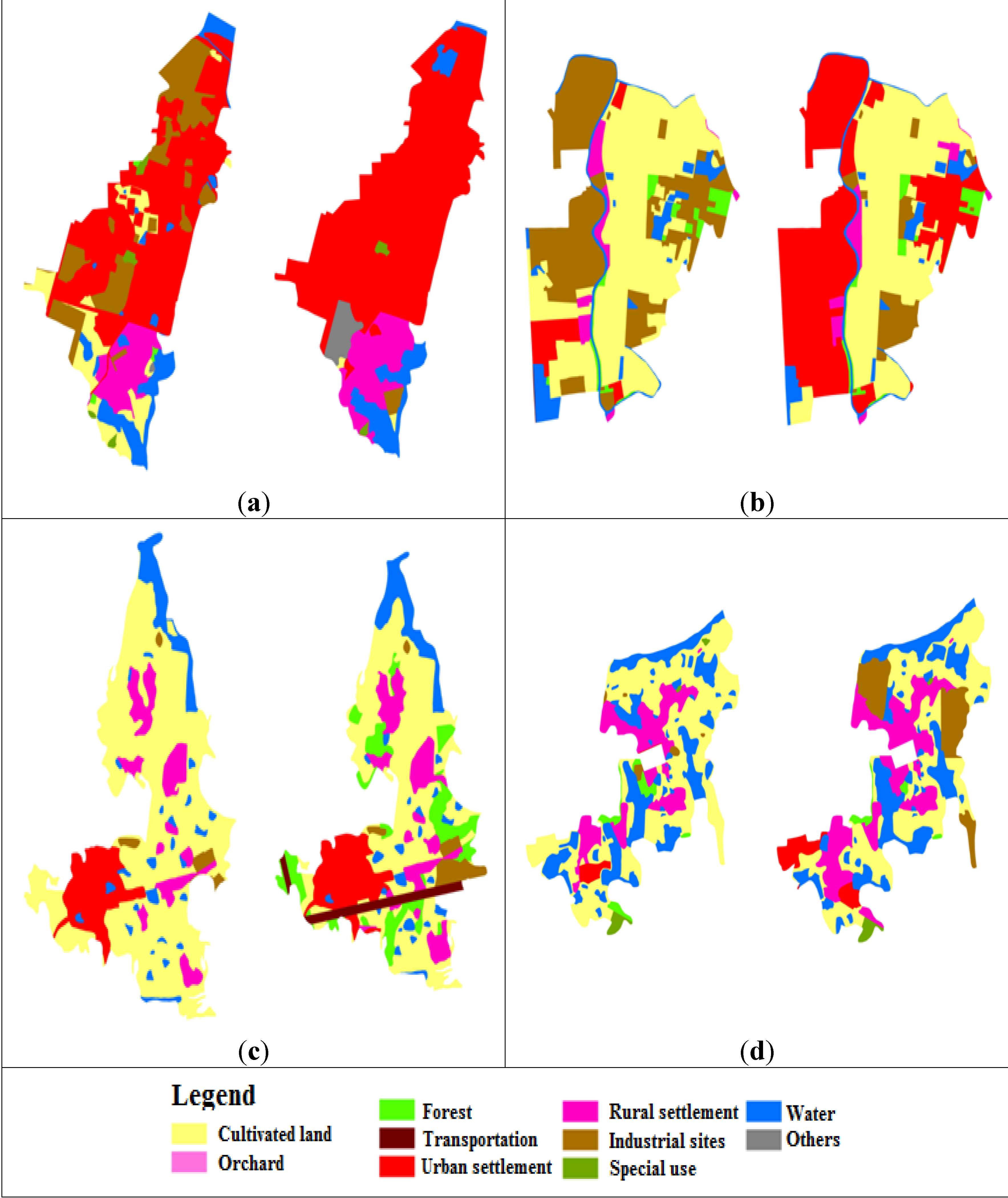
Material used includes land use maps in 1996 and 2006 with attributes of land use type (a derived unified classification system with 25 land use categories), parcel name and other auxiliary information assigned to each patch, Wuhan Geographic Information Blue Book (2006–2011) (WGIBB), China City Statistical Yearbook (1984–2010) and Wuhan Statistical Yearbook (1995–2010). Parcel here is classified by the ownership of land; therefore it is not a homogeneous individual unit in terms of land use type, but an aggregate unit with different type of patches (Figure 2). Four categories are defined as built-up land for analysis: settlements (city and town), roads (railway, highway, and other roads), industrial sites and built-up land for special use such as parks and military occupancy.
Figure 2. Framework of a multi-level and multi-dimensional characterization (Abbreviations for the metrics would be used in the following part; the symbol “*” in metrics represents the metric which is not present at all the levels).
Sustainability 06 03571 g002

3. Multi-Level and Multi-Dimensional Metrics

Metrics are devised in a multi-level manner through a bottom-up approach and the criterion for the selection of levels is their relevance to local and regional jurisdictions where decisions regarding planning and development options occur [33]. At each level, the criterion for the selection of metrics is that they are quantitative and extensive enough to exhibit most of the characteristics with respect to land use, landscape structure, urban form and socio-economic development. The specifications of metrics in each dimension for each level are list in Figure 2 and we elucidate the calculation and connotation of each metric in Appendix I.
• Composition
We use composition dimension to describe the change in urban form associated with land resource consumption, as land development is directly contributed to urban sprawl and embodies human socio-economic activities [22,34]. Metrics applied include built-up patch density (BPD), percentage of settlement area (PS), percentage of transportation area (PT), percentage of industrial site (PI), and percentage of built-up land for special use (PBS). At the metropolitan level, percentage of development zones (PDZ) is also taken into account. This indicator is applied to show the proportion of the area of development zones because they are increasingly scattered in many cities and the delineation of development zones has been a crucial tool to propel urban sprawl in China [35].
• Configuration
Configuration metrics derived from landscape ecology such as fragmentation, heterogeneity, diversity, compactness and morphological features are employed [36,37]. Shannon diversity index (SHDI), shape index (SI), contagion index (DCI) and perimeter-area fractal index (PAFRAC) are applied to parcel level. For the contagion index, since our focus is urban built-up land and land use data is in vector format in our study, we propose a derived contagion index (DCI) from the one in landscape ecology Equation (1).
Sustainability 06 03571 i001
where Pi is proportion of land use i for the total area, mi is the total number of adjacencies for land use i and mij is the number of adjacencies between land use type i and land use type j. The range of the DCI is from 0 to 1, when the parcel is a homogenous unit with a single land use type, the value of DCI is 1 and the lower the value is, the more dispersed distribution of this land use type. Apart from that, Shannon entropy and spatial autocorrelation index (MI) are included to quantify the distribution of built-up land and the degree of decentralization at district and metropolitan level [38]. The specifications of SE and MI are explained in the appendix attached Appendix I.
• Density
We take density as a manifestation of population and economic input and output in relation to land consumption in urban sprawl [39,
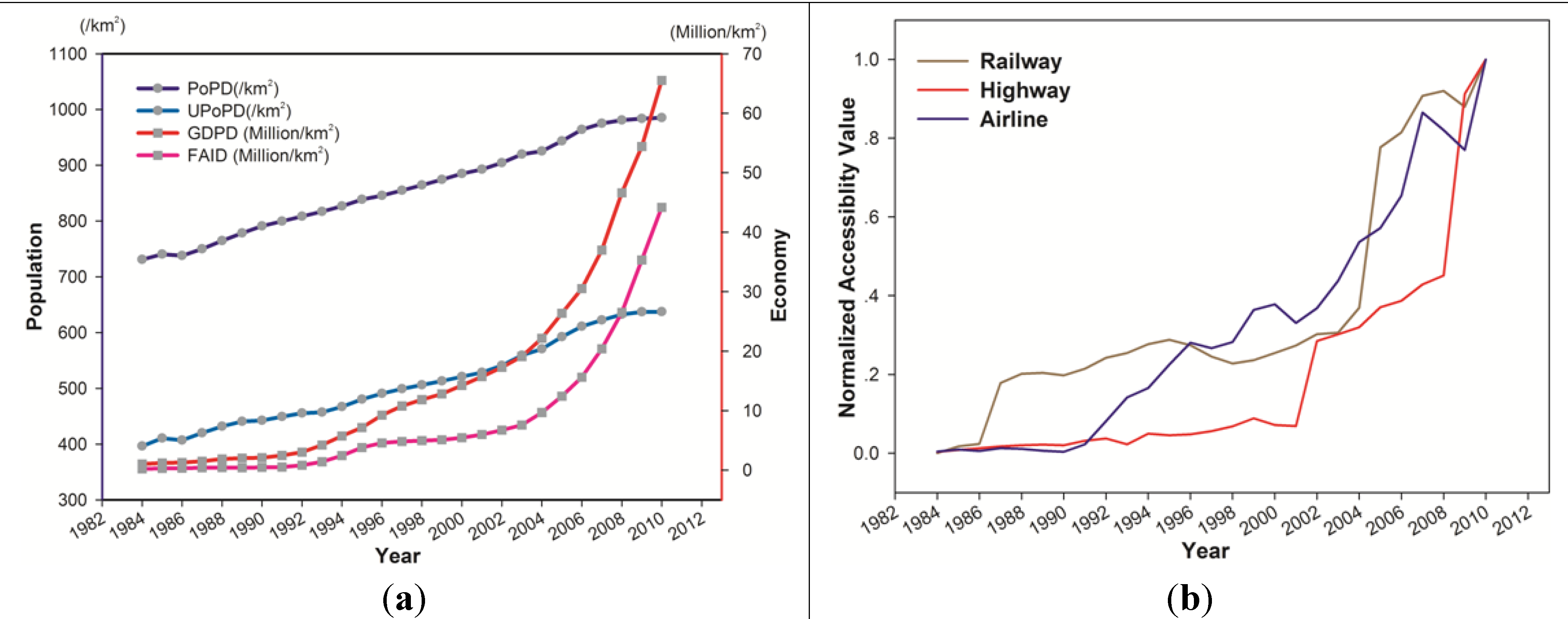
40]. As socio-economic activities are orderly organized and administered at district and metropolitan area levels and aggregated statistical data are available, we introduce population, non-agricultural population, GDP and fixed assets investment for the measurement in density dimension at these two levels. Unlike the per capita indices, we relate them to land consumption by dividing them to the total land area to produce the metrics of PopD, UPopD, GDPD and FAID.
• Gradient
The previous gradient analysis illuminates the spatio-temporal dynamics of built-up land or relevant landscape metrics [25,
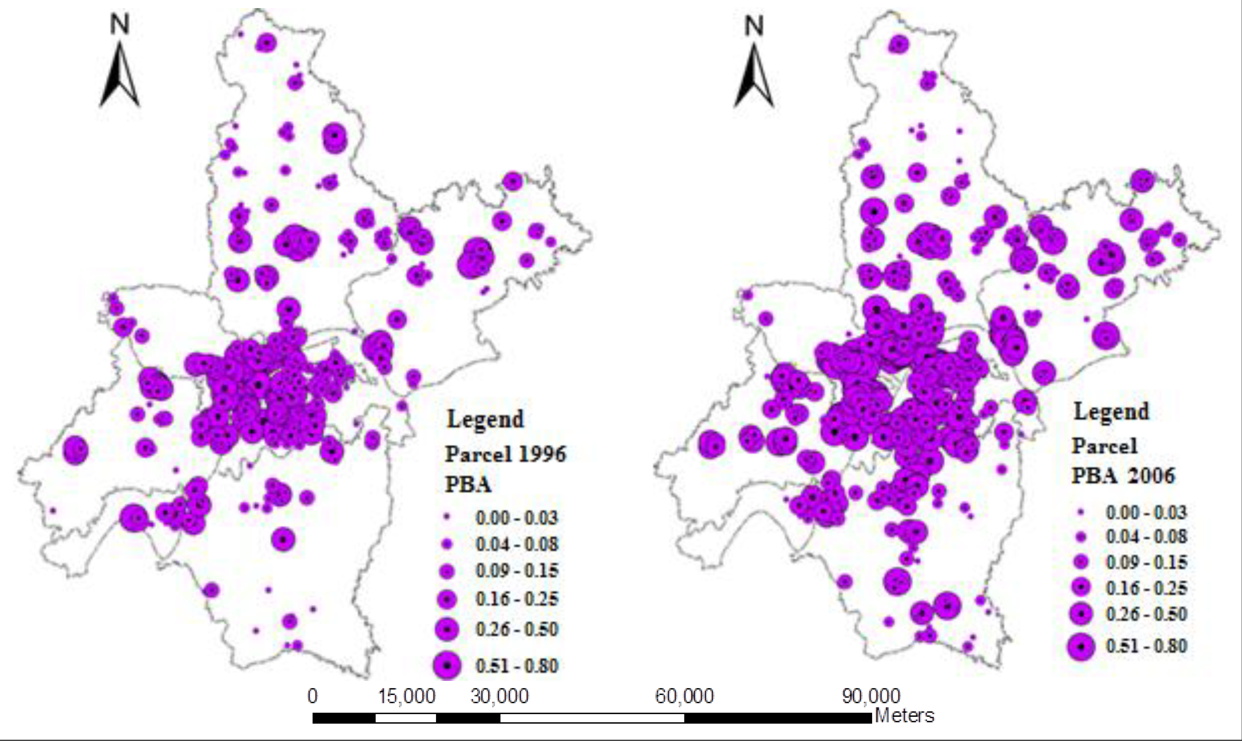
41]. In our research, gradient is designed at the micro-level to depict the sensitivity of urban built-up land to the distance to urban core center. The study area is divided into eight concentric circles of 10 km incrementing radius for analysis. To guarantee the number of parcels in correlation analysis, circles have been aggregated into four zones: <10 km, [10 km, 20 km], [20 km, 40 km], >40 km in 1996 and five zones: <10 km, [10 km, 20 km], [20 km, 30 km], [30 km, 50 km], >50 km in 2006. For each ring, there are at least 80 urban parcels for the estimation of area-distance correlation coefficient (ADC) and density-distance correlation coefficients (DDC).
• Proximity
Proximity to highway, to city center, to CBD and major infrastructures are empirically verified as the major determinants for land development, although not all of them are essential in the multi-polar space [42,43]. We therefore adopt the average distance from each parcel to the weighted centroid of each district to measure proximity at the district level. This is accomplished by first of all, the calculation of settlement centroid, transportation centroid for each district and built up land centroid as the city center based on gravity model (Equation (2)). Secondly, the estimation of average distance as specified in (Equation (3)).
Sustainability 06 03571 i002
Sustainability 06 03571 i003
where Xi and Yi is the coordinates of parcels in a specific district and wi is assigned by the percentage of settlement area, the percentage of transportation area or the percentage of built-up land area in different cases. In Equation (3), (Xs, Ys) is the coordinate of the settlement gravity center to produce ProSub. Similarly, ProTP and ProC are produced according to Equation (3) with the substation of transportation centroid (XT, YT) or built-up land centroid (XC, YC) to settlement centroid (XS, YS). N is the number of parcels in the districts.
• Accessibility
Proximity and accessibility are similar in the sense that they both measure the efficiency of spatial interactions and degree of convenience [31,44]. High level of accessibility also implies short average trip length, commute time and better transportation environment [45,46]. We herein interpret accessibility as the reflection of transportation efficiency and capacity, and design three metrics: comprehensive highway index (CHI), comprehensive railway index (CRI) and comprehensive aviation indices (CAI) (Equation (4)).
Sustainability 06 03571 i004
VHDP and VHDF are the standardized values calculated from two indicators—“Freight ton kilometers” and “passenger kilometers” recorded in the Statistical Yearbook of Wuhan through max-min normalization to the range [0,1]. The same method is also applied to railway and aviation to produce the dataset of CRI and CAI.
• Dynamics
Dynamics exist among all these dimensions and we define it as the centroid migration for probing into the temporal and spatial variation of urban patterns in a comprehensive manner [47]. As described in the proximity dimension for the estimation of settlement and transportation centroids for district, we calculate these centers at the metropolitan area level as well. Then centroid migration is estimated as specified in (Equation (5)).
Sustainability 06 03571 i005
(XS1, YS1) and (XS2, YS2) are the coordinates of settlement centroids in 1996 and 2006 respectively and then the settlement migration distance SCM is obtained. The transportation migration distance TCM can also be estimated accordingly.

4. Sprawling Pattern at Parcel, District and Metropolitan Level

4.1. Sprawling Measurement of Parcels

There are 405 parcels in 1996 and 581 parcels in 2006 with urban settlement, which we take as urban parcels for analysis. Table 1 shows the average values of the composition and configuration metrics at the parcel level. Although the number of parcels with urban settlement has increased during the past ten years, built-up patch density (BPD) has decreased from 27.92 to 17.48. This implies that urban built-up land has been more homogeneous in parcels; at the same time, SHDI has increased from 1.189 to 1.199, indicating land use has been slightly more diversified. Metrics in the composition dimension have all presented a growth trend and settlement forms the largest proportion whereas industrial sites increase most rapidly from 1996 to 2006. Through the calculation of SI and PAFRAC in configuration dimension, it is found that shapes have been more regular and the space has been more filled (more compact) at the parcel level. It is also revealed that parcels at the urban fringes show higher SHDI and lower PAFRAC with the implication of higher fragmentation. Table 2 records the result of contagion metrics for all the built-up land types. All of them have been in a more compact distribution and industrial sites have changed the most from 1996 to 2006.
Table 1. Result of composition and configuration metrics.
MetricsBPD(/km2)PSPTPIPBSSHDISIPAFRAC
199627.92228.73%0.99%4.38%0.70%1.1891.8551.556
200617.47936.32%1.39%6.69%0.90%1.1991.6551.551
Table 2. Result of contagion indicator.
Contagion IndexSub-classification of built-up land
RailwayHighwayUrban settlementsTownsIndustrial sitesBuilt-up land for special use
19960.6460.6550.6300.6330.5890.572
20060.6900.6770.6800.6810.6500.633
More or less++++++
Table 3 shows the result of gradient analysis and it is found that the percentage of built-up land area (PB) and built-up land density (BD) are more sensitive to distance to the city center in 2006 than that in 1996. PB is also found to be more sensitive to distance than built-up density in 1996, though this difference has shrank in 2006. It is also interesting to discover the alternation of positive and negative correlation coefficient between PB or BD and distance, with the implication of the sprawling process and the interaction of centripetal and centrifugal forces as the distance from city center to the urban fringe increases.
Table 3. Result of gradient dimension.
Distance from city center (km)
10204070
96PBA0.033−0.104−0.110.075
96PBN−0.0530.0070.010.023
1020305070
06PBA−0.186−0.064−0.148−0.0510.005
06PBN−0.07−0.0240.0350.2230.025
Figure 3 illustrates the percentage of built-up area in urban parcels in a classified manner. An apparent growth around the periphery of the urban core area has been identified, either in a continuous expanding patter or in a leapfrogged sprawling pattern.
Figure 3. Spatial distribution of the percentage of built-up area at the parcel level (Parcel is stored in land use database with the land use ownership as the identification attribute; urban parcel is defined by the judgment on whether the parcel has urban settlement).
Sustainability 06 03571 g003
We also extract 232 urban parcels simultaneously present in the dataset in 1996 and 2006 for comparison. Change ratio (CR) is calculated by the difference of values in 1996 and 2006 divided by the average of their values. The range of CR is from −200% to 200%. Table 4 and Table 5 exhibit CR of composition and configuration metrics from 1996 to 2006 respectively. The proportion of CR with the value more than 100% approximates to 40% in PT, which is the largest among all the metrics in the composition dimension; whereas the proportion of negative CR is a little less than 20% in PS, which is the least. The change of SHDI is much greater than that in PAFRAC, while the largest proportion of CR comes to the range from −10% to 10% for SI and PAFRAC. Specifically, 65 parcels are diagnosed to increase more than 100% in terms of CR for PS and they are mostly distributed in the range of ring 2, ring 3 and ring 4. Parcels in the north and east appear to be lack of transport construction and PBS is also found to grow more than 100% most likely in ring 3 and ring 4 (rings are divided as described in gradient calculation in Section 2).
Table 4. Change ratio of composition metrics from 1996 to 2006.
Change Ratio IntervalPBNSDTDIDODG
< −100%4.55%7.95%7.85%28.93%31.40%
−100% ≤ CR ≤ 035.64%0.52%1.34%10.64%7.95%
CR = 07.85%72.31%76.55%9.19%23.35%
0 ≤3CR ≤ 100%41.32%0.83%1.34%10.95%7.54%
CR ≥ R100%10.64%18.39%12.91%40.29%34.50%
Table 5. Change ratio of configuration metrics from 1996 to 2006.
Change Ratio IntervalSHDISIPAFRAC
< −100%26.03%29.86%12.81%
−100% ≤ CR ≤ 012.91%23.35%33.06%
0 ≤ CR ≤ 100%15.29%23.45%39.88%
100% ≤ CR ≤ 200%12.40%10.54%10.95%
CR ≥ 200%33.37%12.81%3.31%
As aforementioned, since villages are distributed both in urban and rural areas, it is hard to define urban parcel, as a result, we include all the parcels with urban settlement for the analysis at the parcel level. Built-up land here refers to urban settlement, transportation, industrial sites and land for special use. Figure 4 maps land use changes in four typical parcels. It implies a continuous development of urban settlement, declining trend of parcel number and the loss of farmland. Specifically, newly development roads appear to connect urban settlement and industrial sites (Figure 5c), industrial sites are distributed in a dispersed manner and new constructions are primarily realized by occupying cultivated land (Figure 5a,d), and abandoned industrial land is likely to be transformed to urban settlement (Figure 5b).
From what we have observed, urban areas mainly sprawled through both the infilling process and the outlying expansion at the parcel level. Most newly appeared urban parcels are around the intersection part between city core and suburban districts. In the urban parcel, however, the distribution of built-up land has been more compact. Sprawl, in this case, is realized primarily by merging patches with the same land use type as well as expanding, which is especially true for industrial sites and settlement. On the whole, a key factor to determine whether the urban parcel is sprawled or not is its distance to the city center, which has become increasingly important from 1996 to 2006.
Figure 4. Land use change in four typical urban parcels from 1996 to 2006; (a) Village of SHI LI PU in 1996 and 2006 (b) Faculty of Agricultural Sciences in 1996 and 2006; (c) Village of Da Ji in 1996 and 2006; (d) Village of Jia Ling in 1996 and 2006.
Sustainability 06 03571 g004
Figure 5. The Change Value of metrics for each district from 1996 to 2006 (Color ramp represents the change of each metric in each district and the symbol size refers to the value of each metric in 2006). (a) Change of built-up land patch density (BPD); (b) Change of percentage of settlement area (PS); (c) Change of percentage of transportation area (PT); (d) Change of percentage of industrial site (PI); (e) Change of Percentage of built-up land for special use (PBS); (f) Change of Shannon diversity index (SHDI); (g) Change of shannon Entropy (SE); (h) Change of shape index (SI); (i) Change of perimeter-area fractal index (PAFRAC); (j) Change of spatial autocorrelation index (MI); (k) Change of PopD; (l) Change of UpopD; (m) Change of GDPD; (n) Change of FAID; (o) Change ratio of ProC; (p) Change ratio of ProTP; (q) Change ratio of ProSub.
Sustainability 06 03571 g005
Table 6. The value of each metric in the dimensions of composition, configuration, density and proximity in 2006 at the district level.
MetricsUnitCDDXHHNHPJXXZHYHSJAJHQKQSWC
BPD106/m21.611.920.300.911.251.853.263.362.951.483.202.781.38
PS/2.35%2.67%1.59%1.04%1.51%8.56%21.48%10.63%44.31%71.34%62.00%45.48%36.83%
PT/0.86%1.69%0.01%0.51%0.69%0.49%2.81%0.98%3.93%1.47%2.81%0.56%1.35%
PI/4.44%5.21%1.05%1.71%3.40%1.43%10.07%4.97%7.32%0.92%6.22%6.90%5.30%
PBS/0.32%0.93%0.11%0.40%0.68%0.36%0.74%1.07%0.14%18.77%0.42%0.26%0.10%
SHDI/2.372.382.251.712.212.332.272.601.920.971.451.901.49
SE/0.790.780.450.760.780.780.610.750.580.640.660.650.31
SI/1.551.861.991.331.471.441.781.531.892.192.791.662.40
PAFRAC/1.391.371.371.381.381.371.421.401.401.611.441.431.47
CImax/0.96270.87550.79400.67090.70640.80290.89210.79370.70950.99800.82130.77020.9993
CImin/0.50880.69000.58650.50220.49800.51210.89200.60140.56760.96930.50670.76950.9891
MI/0.240.490.240.370.350.380.240.270.26−0.160.460.630.26
PopD/km24015943704923206504845185910,14513,89211,493994813,163
UPopD/km2106190888910314641901469984013,89211,256994313,075
GDPDmilliom/km25.9619.618.454.474.696.08176.5038.02253.69647.35372.82585.74278.93
FAIDmilliom/km22.1715.762.342.082.682.6754.1024.29173.96366.50121.3287.89120.64
ProSubm13,83512,41613,81719,27220,37116,044512913,09836312714254666384641
ProTPm13,593925813,49422,26820,18223,748475412,60037623068283965065445
ProCm33,84626,52047,46944,75337,01150,41412,49215,62510,156800812,59914,2685086

3.2. Sprawling Characteristics for Districts

Table 6 records the value of each metric in the dimensions of composition, configuration, density and proximity in 2006 and Figure 5 illustrates the change of each metric from 1996 to 2006 at the district level. Districts within city center are in a superior position and have experienced greater change; HP and JX which are the largest districts in Wuhan metropolitan area are found to be inferior in density dimension. In 1996, JH exhibited the highest density value and WC developed faster by 2006. During these 10 years, the most obvious increases in population exist in DXH and HS. On the other hand, GDP and fixed asset investment grow fastest in QS and QK respectively. Built-up patch density declines most in WC and the most significant increase occurs in HP. DXH and Hongshan emerge as the fastest growing districts in terms of residential area whereas JX and JA are ranking higher with respect to the increase on transportation area. Industrial areas appear to triple in HN and QK experience the most increase for built-up land for special use. Through the calculation of metrics in configuration metrics, it is found that land use in districts in outer rings is more diversified and more dispersed, than that in the city center, whereas their shapes are more regular [24]. PAFRAC is apparently increasing in the past decade, which implies land use in urban core are more space filled and justifies the response to the proposition and implementation of “Intensive Urban Land Use Strategy” in China [48]. There is not much regular pattern for proximity metrics in temporal terms; however, greater change exists in suburban districts. The results of global Moran’s I reveal that HY in the city center changes from the highest of density of compaction to the most dispersed from 1996 to 2006. It is also found that urban settlements in QK are in the lowest density of compaction in 1996 and other land for transportation in QS is distributed most dispersedly in 2006.
Unlike the sprawling process at the parcel level, the distribution of built-up land has been more scattered at the district level, which is coupled with more fragmented local landscape, in the suburban districts in particular. The distinct gap between urban and suburban areas in terms of density metrics has also been identified and the composition of the land form has changed greater in suburban districts especially in CD and JX. Urban districts in the city core, though also identified with the expansion and the dispersion of built-up land, continues to show an upward trend in density. The emerging suburban districts in the 1990s are the strategically reflection of the policy of transforming county into urban district and urban sprawl there is primarily realized by dispersing settlement, industrial sites as well as built-up land for some special use.

3.3. The Metropolitan Sprawling Trend

Figure 6a shows that the yearly population density and non-agricultural population density present a similar variation from 1984 to 2010 at the metropolitan level. An analogue pattern can also be found in GDP density and FAI density with a gradual growth before 1994 and an exponential increase after 2000. Figure 6b illustrates accessibility metrics measured by the standardized CRI, CHI and CAI, which demonstrates an increasing trend and the growth rate has been considerably higher after 2000.
Figure 6. Temporal change of density and accessibility metrics from 1984 to 2011. (a) Variation in density metrics; (b) Variation in accessibility metrics.
Sustainability 06 03571 g006
Table 7 indicates that, in composition dimension, apart from built-up patch density, all the metrics have showed a remarkable increase, PI and PT in particular, with the implication of a rapid industrialization process and noticeable transportation advancement. Noticeably, there are only two development zones approved by the state council in 1996 with the area of approximately 725 km2. By the year of 2006, three national development zones and 12 provincial development zones have been designated with the total area of 1076.77 km2 and they are more scattered distributed within and around the city center, as displayed in Figure 1.
Table 7. Results for Composition Metrics at the metropolitan level.
BPDPSPTPIPBSPDZ
19961.372.65%0.27%1.68%0.53%8.56%
20061.514.28%0.75%3.00%0.57%12.68%
Through the calculation of configuration metrics, it is found that land use has been more diversified and urban built-up land has been more scattered (Table 8). Shape index has declined and PAFRAC has slightly increased. The results of derived contagion index tell us that the maximally concentrated land use type is settlement in cities and the most scattered is built-up land for special use among all the built-up land use types. The global Moran’s I has increased from 0.22 to 0.36 and maps of LISA (local indicators of spatial association) illustrates that a clear-cut high-high clustering has been statistically significant at the urban core and low-low pattern has been primarily at the suburban fringe both in 1996 and 2006 (Figure 7), which implies the sprawling trend around the periphery of city center.
Table 8. Results for Configuration Metrics at the metropolitan level.
SHDISESICIMaxCIminPAFRACMI
19962.410.71.520.710.551.330.22
20062.550.771.450.750.541.340.36
Figure 7. Spatial autocorrelation of Wuhan Metropolitan area (the unit for spatial autocorrelation analysis is parcel).
Sustainability 06 03571 g007
Table 9 describes values of the metrics in the dimensions of proximity and dynamics dimension. It is shown that proximities to settlement, transportation and city center have increased slightly and dynamically, urban settlement centroid has migrated 4965.11 m to southwest and in the same direction the shifting distance is 2437.14 m for transportation centroid.
Table 9. Results for Proximity and Dynamics Metrics at the metropolitan level.
ProximityDynamics
ProSubProTPProCSCMTCM
199637,772.9137090.6937,976.134965.112437.14
200637,995.39937,568.87938,132.037(Southwest)(Southwest)
The Wuhan metropolitan area is also diagnosed as sprawl since urban built-up land has increased and their distribution is has become more scattered, which is similar with that at the district level. Density and accessibility, on the other hand, have also grown tremendously in the past twenty years, which is another evidence of the co-existence of sprawl and compact development. Noticeably, urban sprawled towards southwest and the area of development zones have expanded with more than 300 km2 at the peripheral areas between city center and suburban district.

5. Discussion and Implications

At the beginning of this study, we raised two questions on how to establish a hierarchical measurement and how to choose appropriate metrics at each level to improve the practicality of the measurement and to realize the sustainable urban development. The first issue is resolved by devising the metrics at three levels: micro-level (parcel), meso-level (urban district) and macro-level (metropolitan area). For characterizing urban sprawl in a metropolitan area, macroscopic measurement is suitable for tracing the comprehensive development, however, this may result in great deficit information and a sprawled pattern for a metropolitan area can be heterogeneous at the intra-urban level such as district or other subsidiary administrative units. Highly disaggregate, georeferenced data on land use, together with the power of Geographic Information System (GIS), have enabled researchers in recent years to embark on quantifying fine-scale characteristics of urban land use pattern [31]. The employment of parcel and urban district as the levels for carrying out the multi-level measurement is highly novel and beneficial. Land is one of the fundamental aspects reflecting the administrative decentralization and the revitalization of the land market has necessitated the control of urban sprawl to be implemented at the bottom parcel level. By identifying parcels with great changes in relate to land resources, policy makers can formulate adaptable regulations for those land owners. We have illustrated the internal land use changes in four typical parcels and the most prominent problem is still the occupation of cultivated land as the cost of the expanding built-up land. As a result, the farmland protection policies need to be reinforced, especially at the finer scale such as parcel. Urban districts could be regarded as a medium and transitive level as a certain degree of autonomous right for regulating land use exist at this level. In the first section, we mentioned the strategy of “transforming county into urban district” which strengthens the importance of investigating its socio-economic and spatial structure as their change is the most straightforward reflection of urban sprawl. Two of the six urban districts in the vicinity are transformed from counties and the striking disparity is observed between the six urban districts at suburban areas and the seven urban districts in the city center. Measurements at this level lay the foundation of formulating policies such as mitigating population density, controlling the expansion of residential area and curbing the expansion of industrial sites in central district such as JH. On the contrary, development in suburban districts such as HP, HN and JX should be considered to be strengthened in terms of financial support and infrastructure construction. Meanwhile, urban settlement is further scattered in districts outside the city center such as HP and JX and a more compact spatial restructuring is expected to be implemented in the future.
Then we move to the second aspect on the selected dimension and metrics as well as their relevance and representativeness to the three levels. These 28 metrics in seven dimension can be generally categorized into three groups—one referring to metrics present in all the three levels, one is the metric only exists at the parcel level and the last group includes metrics characterizing urban sprawl at the urban district and metropolitan level. For the first group, metrics are primarily similar with those in landscape ecology functioning in the manifestation of the composition and configuration in certain areas. There exists scale effect here; even the parcel is located in a certain urban district, the values for this parcel and for this urban district can be of great difference in composition and configuration dimension. Meanwhile, the temporal variation can also be scale-sensitive. This spatio-temporal heterogeneity is what we expected to be useful for providing policy implications at the finer scale in intra-urban development. Another group exclusively pertaining to parcel level is the gradient dimension embracing two metrics ADC and DDC. This is a special dimension as it actually expresses the overall spatial change, though the variable herein is affiliated to parcel. The gradient metrics—ADC and DDC demonstrate the spatial distribution of the parcels reflecting the circle layer structure in a specific area. This helps to probe into the sprawling process and spatial changes not abided by the rule of economic geography may threaten the urban sustainability. The last group is those dimensions and metrics devised for urban districts or metropolitan area. We employ more socio-economic metrics as well as spatio-temporal explicit metrics to capture the multi-faceted features of urban sprawl. As a matter of fact, when the small units are aggregated to a higher level, more complicated sprawl pattern or associated socio-economic development emerge. For example, PDZ is exclusively used at the metropolitan level as the development zones may span a dozen of parcels or adjacent districts and proximity allows us to judge the settlement or transportation distribution. As a result, it is difficult to distinguish one dimension or metric from others as each of them possess specific function to reveal the magnitude, pattern, direction or the dynamics of urban sprawl at different levels.
In general, the superiorities of our approach are first of all, to understand the scale-effect and explore the intra-urban changes in the context of notable urban sprawl. Since we have hundreds of parcels and 13 districts, we get the average value of different metrics and make comparisons. Most of the metrics vary in the same direction at different levels except PBS, FI and ProSub from 1996 to 2006. PBS grows at the parcel and metropolitan level while a downward trend appears at the district level; ProSub rises at the district level and declines at the metropolitan area level. FI has been mentioned in the previous paragraph. This has potential link to the scale-effect in urban planning which is largely negligible in the past and it is rendered potential recommendations to the spatial urban planning for land use and infrastructure construction. Second, the devising of the metrics is conformed to the principles of suitability, quantitativeness and feasibility, which makes us understand the pattern, the process and the magnitude of the sprawl in a comprehensive manner. It is noticeable that there are differences in matching metrics to different levels because adjustments would help to demonstrate their own characteristics. For example, MI appear at the district and metropolitan level but not at the parcel level, which is due to the fact that not all the parcels are with high complexity to demonstrate spatial concentration or decentralization. Meanwhile, our systematic measurement framework is easy to be implemented for other cases as it is not highly data-demanding. Third, in order to curb urban sprawl, a bottom-up approach is more operational with the strengths in policy making and implementation, especially when levels are corresponding to China’s administrative hierarchy [49,50]. Although a mass of literatures have mentioned the problem that scientific research, to a large extent, is scrambling to taking into effect for governors or administrators, there still appears to be lack of solutions. This is the same case in urban sprawl. In the sense of hierarchical urban administration, a metropolitan area is composed of districts or counties which are comprised by a number of parcels. The decentralization in controlling urban sprawl can thus be accomplished from parcels, where land is allotted to owners for use. The micro-level measurement together with the integration of aggregated district and metropolitan levels is beneficial for guiding the formulation of strategic management and planning policies.

6. Conclusions

In this research, we have performed the characterization and measurement of urban sprawl in a multi-level and multi-dimensional manner. On one hand, the results of the metrics applied in Wuhan back up the assertion that Chinese cities are tending to present mixed sprawling patterns with randomly expansion at urban fringe, strip development along or between highways, scattered and leapfrog development of industrial land and continuous development of urban residence [6,51]. Apparent expansion is identified around the periphery of urban centers at all these three levels with higher degree of dispersion, which is largely attributed to the policy-oriented development such as setting up various development zones, industrial parks or by delineating “Jianchengqu” [11,17,52]. On the other hand, we have drawn three major conclusions methodologically:
(1)
This multi-level approach, which is parcel at micro-level, district at meso-level and metropolitan area at macro-level, is capable of identifying the scale-effect in urban sprawl and its spatio-temporal variation at finer scales. It allows a thorough understanding on the urban spatial structure as well as the socio-economic development. In particular, the investigation on parcels is novel and of great pragmatic values for better regulation on urban sprawl at finer scales. In addition, the scale-effect unearthed from the multi-level measurement provides substantial evidence to the importance of scale in urban planning and implicate the adjustment of land use and infrastructure construction in the near future.
(2)
The multi-dimensional characterization, which is categorized as composition, configuration, gradient, density, proximity, accessibility and dynamics, justifies the sprawling process by identifying the expansion of built-up land and dispersed distribution. It is revealed that industrial sites and built-up land for special use are found to be most scattered and randomly distributed, parcels and districts at the urban fringe present higher fragmentation than those in the urban core areas and urban expansion is enforced by assigning development zones or delineating Jianchengqu. Specifically, apart from measuring sprawling pattern in the whole metropolitan area, we also identified parcels or districts with great changes from 1996 to 2006 from dimensions which can facilitate the institutional management.
(3)
In addition, the integration of multi-dimensional and multi-level framework can be of great extendibility and feasibility. Additional metrics or dimensions can be easily embedded when relevant data or information are collected. Levels are not necessarily confined to aggregated units described above, but are determined in the consideration of city management and planning, hierarchical administration, data availability, etc. The framework we established and implemented here has proved to be effective for the exploration of the spatio-temporal variation of intra-urban pattern and provide reference for the administrators or policy makers in a pragmatic manner.

Acknowledgments

The authors would like to thank Elisabete Silva from University of Cambridge, James P. LeSage from Texas State University, and some other staff from Science from Key Laboratory of Geographical Information Sciences in Wuhan University for their help and suggestions in this research. The author would also be grateful for the support from the Fundamental Research Funds for the Central Universities (52902-0900206135).

Author Contributions

The first and corresponding author-Chen Zeng wrote the paper and designed the research. The second author Sanwei He co-designed the research and made detailed revisions. The third author Jiaxing Cui processed and analyzed the data. All authors read and approved the final manuscript.

Conflicts of Interest

The authors declare no conflict of interest.

Appendix I

Composition:
(1)
Built-up land patch density (BPD): Sustainability 06 03571 i101
NBP is number of built-up land patches; A is area of the parcel;
Units: IND/km2; Range: BPD > 0, without limit;
Description: Built-up land patch density is a limited, but fundamental, aspect of landscape pattern. It expresses number of patches with built-up land attribute on a per unit area basis that facilitates comparisons among landscapes of varying size.
(2)
Percentage of settlement area (PS): Sustainability 06 03571 i102
As is the area of settlements in a parcel; A is area of the parcel;
Units: Percentage; Range: 0 ≤ PS ≤ 1;
Description: Percentage of settlement area quantifies the proportional abundance of settlement patch type in the landscape. It is a relative measure of landscape composition important in many ecological applications.
(3)
Percentage of transportation area (PT): Sustainability 06 03571 i103
AT is the area of transportation land in a parcel; A is area of the parcel;
Units: Percentage; Range: 0 ≤ PT ≤ 1;
Description: Percentage of transportation area quantifies the proportional abundance of transportation patch type in the landscape. It is a relative measure of landscape composition important in many ecological applications.
(4)
Percentage of industrial site (PI): Sustainability 06 03571 i104
AI is the area of industrial land in a parcel; A is area of the parcel;
Units: Percentage; Range: 0 ≤ PI ≤ 1;
Description: Percentage of industrial site quantifies the proportional abundance of patch type with industrial land attribute in the landscape. It is a relative measure of landscape composition important in many ecological applications.
(5)
Percentage of built-up land for special use (PBS): Sustainability 06 03571 i105
ASU is the area of open space and green space in a parcel; A is area of the parcel;
Units: Percentage; Range: 0 ≤ PBS ≤ 1;
Description: Percentage of built-up land for special use quantifies the proportional abundance of patch type with built-up land for special use attribute in the landscape. It is a relative measure of landscape composition important in many ecological applications.
(6)
Percentage of development zones (PDZ) : Sustainability 06 03571 i106
ADZ is the area of development zones; A is area of the parcel;
Units: Percentage; Range: 0 ≤ PDZ ≤ 1;
Description: Percentage of development zones quantifies the proportional abundance of the area of development zones in the landscape. It is a relative measure of landscape composition and applied to the measurement at the metropolitan level.
Configuration:
(1)
Shannon diversity index (SHDI)
SHDI is the area of open space and green space in a parcel; A is area of the parcel;
Units: Percentage; Range: 0 ≤ PBS ≤ 1;
Description: Percentage of built-up land for special use quantifies the proportional abundance of patch type with built-up land for special use attribute in the landscape. It is a relative measure of landscape composition important in many ecological applications.
(2)
Shape index (SI): Sustainability 06 03571 i107, Pij is the perimeter (m) of patch ij; aij is the area of patch ij; k is the number of patches in each parcel/district/metropolitan area;
Units: None; Range: 1 ≤ SI;
Description: Shape index reflects shape complexity across a range of spatial scales. SI approaches 1 for shapes with very simple perimeters such as squares, and the larger the values are, the higher degree of irregular shape it is of.
(3)
Shannon Entropy (SE): Sustainability 06 03571 i108
Units: None; Range: 0 ≤ SI ≤ 1;
Description: If the distribution of built-up land is maximally concentrated in a single cluster, then SE = 0, whereas if it is evenly distributed among the clusters, SE = 1.
(4)
Contagion index (DCI): Sustainability 06 03571 i001
where Pi is proportion of land use i for the total area, mi is the total number of adjacencies for land use i and mij is the number of adjacencies between land use type i and land use type j.
Units: None; Range: 0 ≤ DCI ≤ 1;
Description: DCI approaches 0 when the patch types are maximally disaggregated (i.e., every unit is a different patch type) and interspersed (equal proportions of all pairwise adjacencies). CONTAG = 1 when all patch types are maximally aggregated; i.e., when the landscape consists of single land use type. Low levels of patch type dispersion (i.e., high proportion of like adjacencies) and low levels of patch type interspersion (i.e., inequitable distribution of pairwise adjacencies results in high contagion, and vice versa. This is derived from the CONTAG metric in Fragstats.
(5)
Perimieter-area fractal index (PAFRAC):
Sustainability 06 03571 i110,
Pij is the perimeter (m) of patch ij; aij is the area of patch ij, N is the total number of patches in the landscape. M is the number of land uses i in the study area; n is the number of patches j.
Units: None; Range: 1 ≤ FI ≤ 2;
Description: Perimeter-area fractal dimension is a metric of space-filling between one- (unfilled) and two- (the fully-compact city) dimensions. Growth in fractal dimension over time is illustrative of compaction; decline suggests fragmentation. Fractal dimension measures have the added benefit of being scale-independent (Torrens, 2008).
(6)
Moran’s I
Sustainability 06 03571 i111
where n is the number of land parcels in the landscape, xi is the percentage of built-up land (PB) for parcel i, xj is the percentage for parcel j, x is the mean value, and wij registers the adjacency between parcel i and j, being the rook continuity option in our case (Lesage, 1999).
Units: None; Range: 0 ≤ MI ≤ 1;
Description: Moran’s I is a spatial autocorrelation metric that measures urban decentralization (Moran, 1950; Torrens, 2008) (Torrens, 2008). Positive values of I indicate land parcels that are more similar in value x than the average y; negative values indicate dissimilarity. A condition of I = 0 indicates an absence of statistically- relevant patterning of value x over i and j.
Density:
(1)
Population density (PopD) Sustainability 06 03571 i112 P is the population of the unit, AS is the area of unit
Units: /km2; Range: 0 ≤ PopD.
Description: It reflects the density of population.
(2)
Non-agricultural population density (UPopD): Sustainability 06 03571 i113 P is the population of the unit, AS is the area of unit
Units: /km2; Range: 0 ≤ UPopD.
Description: It reflects the density of non-agricultural population.
(3)
GDP density (GDPD): Sustainability 06 03571 i114 GDP is the gross domestic product, AS is the area of unit
Units: million/km2; Range: 0 ≤ GDPD.
Description: It reflects the density of economic output.
(4)
FAI density (FAID): Sustainability 06 03571 i115 FAI is the fixed asset investment, AS is the area of unit
Units: million/km2; Range: 0 ≤ FAID.
Description: It reflects the density of fixed asset investment.
Gradient:
(1)
Area-distance correlation coefficient (ADC): ADC = f(Ai, Di), Ai is the area of parcel i and Di is the distance between parcel i to the city center.
Units: None; Range: 0 ≤ ADC ≤ 1;
Description: It depicts the sensitivity of the area of built-up land to the distance to urban core center.
(2)
Density-distance correlation coefficient (DDC): DDC = f(BPDi, Di), BPDi is the built-up land density of parcel i and Di is the distance between parcel i to the city center.
Units: None; Range: 0 ≤ DDC ≤ 1
Description: It depicts the sensitivity of the area of the built-up land density to the distance to urban core center.
Proximity
(1)
Proximity to sub-center (ProSub): Sustainability 06 03571 i118, Xi and Yi is the coordinates of parcels in a specific district. XS and YS is the coordinates of the weighted center of the district and the weights are assigned by the percentage of settlement area in each parcel. N is the number of parcels in the districts.
Units: m; Range: 0 ≤ ProSub
Description: It reflects the proximity to the settlement center.
(2)
Proximity to sub-center (ProTP): Sustainability 06 03571 i119
where XT and YT is the coordinates of the weighted center of the district and the weights are assigned by the percentage of transportation area in each parcel. N is the number of parcels in the districts.
Units: m; Range: 0 ≤ ProSub
Description: It reflects the proximity to the settlement center.
(3)
Proximity to sub-center (ProC): Sustainability 06 03571 i120, Where XC and YC is the coordinates of the weighted center of the district and the weights are assigned by the percentage of built-up land in each parcel. N is the number of parcels in the districts.
Units: m; Range: 0 ≤ ProSub;
Description: It reflects the proximity to the settlement center.
Accessibility
(1)
Comprehensive highway index (CHI): Sustainability 06 03571 i121, VHDP and VHDF are the standardized values calculated from two indicators -“Freight ton kilometers” and “passenger kilometers” recorded in the Statistical Yearbook of Wuhan through max-min normalization with the range from 0 to 1.
Units: none; Range: 0 ≤ CHI ≤ 1;
Description: It reflects the capacity of highway transportation.
(2)
Comprehensive railway index (CRI): Sustainability 06 03571 i122, VRDP and VRDF are the standardized values calculated from two indicators -“Freight ton kilometers” and “passenger kilometers” recorded in the Statistical Yearbook of Wuhan through max-min normalization with the range from 0 to 1.
Units: none; Range: 0 ≤ CRI ≤ 1;
Description: It reflects the capacity of railway transportation.
(3)
Comprehensive aviation index (CAI): Sustainability 06 03571 i123, VADP and VADF are the standardized values calculated from two indicators -“Freight ton kilometers” and “passenger kilometers” recorded in the Statistical Yearbook of Wuhan through max-min normalization with the range from 0 to 1.
Units: none; Range: 0 ≤ CAI ≤ 1;
Description: It reflects the capacity of aviation transportation.
Dynamic
(1)
Migration of settlement center (SCM): Sustainability 06 03571 i124, (XS1, YS1) and (XS2, YS2) are the coordinates of settlement centroids in 1996 and 2006 respectively and then the settlement migration distance SCM is obtained. The transportation migration distance TCM can also be estimated accordingly.
Units: m; Range: 0 ≤ SCM;
Description: It reflects the spatio-temporal variation of settlement distribution.
(2)
Migration of transportation center (TCM): Sustainability 06 03571 i125, (XT1, YT1) and (XT2, YT2) are the coordinates of settlement centroids in 1996 and 2006 respectively and then the settlement migration distance TCM is obtained. The transportation migration distance TCM can also be estimated accordingly.
Units: none; Range: 0 ≤ TCM ≤ 1;
Description: It reflects the spatio-temporal variation of transportation distribution.

References and Notes

  1. Couch, C.; Leontidou, L.; Petschel-Held, G. Urban Sprawl in Europe; Blackwell: Oxford, UK, 2007. [Google Scholar]
  2. Brueckner, J.K. Urban sprawl: Diagnosis and remedies. Int. Reg. Sci. Rev. 2000, 23, 160–171. [Google Scholar] [CrossRef]
  3. Glaeser, E.L.; Kahn, M.E. Sprawl and Urban Growth. In The Handbook of Urban and Regional Economics; Henderson, J.V., Thisse, J.F., Eds.; Oxford University Press: England, UK, 2003; pp. 1–55. [Google Scholar]
  4. Brueckner, J.K.; Mills, E.; Kremer, M. Urban Sprawl: Lessons from Urban Economics. In Brookings-Wharton Papers on Urban Affairs; Gale, W.G., Pack, J.R., Eds.; Brookings Institution Press: Washington, DC, USA, 2001; pp. 65–97. [Google Scholar]
  5. Deng, F.; Huang, Y. Uneven land reform and urban sprawl in China: The case of Beijing. Progr. Plann. 2004, 61, 211–236. [Google Scholar] [CrossRef]
  6. Liu, J.; Zhan, J.; Deng, X. Spatio-temporal patterns and driving forces of urban land expansion in China during the economic reform era. Ambio 2005, 34, 450–455. [Google Scholar]
  7. Ding, H.; Wang, R.C.; Wu, J.P.; Zhou, B.; Shi, Z.; Ding, L.X. Quantifying land use change in Zhejiang Coastal Region, China using multi-tem- poral Landsat TM/ETM+ Images. Pedosphere 2007, 17, 712–720. [Google Scholar] [CrossRef]
  8. Shi, L.Y.; Shao, G.F.; Cui, S.H.; Li, X.; Lin, T.; Yin, K.; Zhao, J. Urban three-dimensional expansion and its driving forces-A case study of Shanghai, China. Chin. Geogr. Sci. 2009, 19, 291–298. [Google Scholar] [CrossRef]
  9. Lu, Z.; Dai, F.; Sun, C. Evaluation of urban sprawl and urban landscape pattern in a rapidly developing region. Environ. Monit. Assess. 2012, 184, 6437–6448. [Google Scholar] [CrossRef]
  10. Camagni, R.; Gibelli, M.C.; Rigamonti, P. Urban mobility and urban form: The social and environmental costs of different patterns of urban expansion. Ecol. Econ. 2002, 40, 199–216. [Google Scholar] [CrossRef]
  11. Zeng, C.; Liu, Y.; Liu, Y.; Qiu, L. Urban sprawl and related problems: Bibliometric analysis and refined analysis from 1991 to 2011. Chin. Geogr. Sci. 2014, 24, 1–13. [Google Scholar] [CrossRef]
  12. Wu, F.; Xu, J.; Yeh, A.G.O. Urban Development in Post-Reform China: State, Market, and Space; Taylor&Francis: Abingdon, UK, 2007. [Google Scholar]
  13. Ma, Y.; Xu, R. Remote sensing monitoring and driving force analysis of urban expansion in Guangzhou City, China. Habit. Int. 2010, 34, 228–235. [Google Scholar] [CrossRef]
  14. Ho, S.P.S.; Lin, G.C.S. Converting land to nonagricultural use in China’s coastal provinces. Mod. China 2004, 30, 81–112. [Google Scholar] [CrossRef]
  15. Tan, M.H.; Li, X.B.; Xie, H.; Lu, C.H. Urban land expansion and arable land loss in China—A case study of Beijing-Tianjin-Hebei region. Land Use Policy 2005, 22, 187–196. [Google Scholar]
  16. Han, J.; Hayashi, Y.; Cao, X.; Imura, H. Application of an integrated system dynamics and cellular automata model for urban growth assessment: A case study of Shanghai, China. Landsc. Urban Plann. 2009, 91, 133–141. [Google Scholar] [CrossRef]
  17. Zhang, T. Land market forces and government’s role in sprawl. Cities 2000, 17, 123–135. [Google Scholar] [CrossRef]
  18. Yeh, A.; Wu, F. The new land development process and urban development in Chinese cities. Int. J. Urban Reg. Res. 1996, 20, 330–353. [Google Scholar] [CrossRef]
  19. Zhou, Y.X.; Ma, L.J.C. Economic restructuring and suburbanization in China. Urban Geogr. 2000, 21, 205–236. [Google Scholar] [CrossRef]
  20. Bhatta, B.; Saraswati, S.; Bandyopadhyay, D. Urban sprawl measurement from remote sensing data. Appl. Geogr. 2010, 30, 731–740. [Google Scholar] [CrossRef]
  21. Balaban, O. The negative effects of construction boom on urban planning and environment in Turkey: Unraveling the role of public sector. Habit. Int. 2012, 36, 26–35. [Google Scholar] [CrossRef]
  22. Yue, W.Z.; Liu, Y.; Fan, P.L. Measuring urban sprawl and its drivers in large Chinese cities: The case of Hangzhou. Land Use Policy 2013, 31, 358–370. [Google Scholar] [CrossRef]
  23. Hasse, J.E.; Lathrop, R.G. Land resource impact indicators of urban sprawl. Appl. Geogr. 2003, 23, 159–175. [Google Scholar] [CrossRef]
  24. Torrens, P.M. A toolkit for measuring sprawl. Appl. Spat. Anal. Policy 2008, 1, 5–36. [Google Scholar] [CrossRef]
  25. Salvati, L.; Zitti, M.; Sateriano, A. Changes in city vertical profile as an indicator of sprawl: Evidence from a Mediterranean urban region. Habit. Int. 2013, 28, 119–125. [Google Scholar] [CrossRef]
  26. Yu, X.J.; Ng, C.N. Spatial and temporal dynamics of urban sprawl along two urban-rural transects: A case study of Guangzhou, China. Landsc. Urban Plann. 2007, 79, 96–109. [Google Scholar] [CrossRef]
  27. Liu, J.; Zhang, Z.; Xu, X.; Kuang, W.; Zhou, W.; Zhang, S.; Li, R.; Yan, C.; Yu, D.; Wu, S.; et al. Spatial patterns and driving forces of land use change in China during the early 21st century. J. Geogr. Sci. 2010, 20, 483–494. [Google Scholar] [CrossRef]
  28. Zhao, P. Managing urban growth in a transforming China: Evidence from Beijing. Land Use Policy 2011, 28, 96–109. [Google Scholar] [CrossRef]
  29. Millward, H. Urban containment strategies: A case-study appraisal of plans and policies in Japanese, British, and Canadian cities. Land Use Policy 2006, 23, 473–485. [Google Scholar] [CrossRef]
  30. Huang, B.; Zhang, L.; Wu, B. Spatio-temporal analysis of rural-urban land conversion. Int. J. Geogr. Inf. Sci. 2009, 23, 1–27. [Google Scholar] [CrossRef]
  31. Irwin, E.; Bockstael, N.; Cho, H. Measuring and modeling urban sprawl: Data, scale and spatial dependencies. In Draft for 53rd Annual North America Regional Science Association of Regional Science Association International, Toronto, ON, Canada, 2006; North America Regional Science Association of Regional Science Association International.
  32. Ali, R.; Zhao, H. Wuhan, China and Pittsburgh, USA: Urban environmental health past, present and future. Ecohealth 2008, 5, 159–166. [Google Scholar] [CrossRef]
  33. Hepinstall, C.J.; Coe, S.; Hutyra, L.R. Urban growth patterns and growth management boundaries in the Central Puget Sound, Washington, 1986–2007. Urban Ecosyst. 2013, 16, 109–129. [Google Scholar] [CrossRef]
  34. Abdulaal, W.A. Large urban developments as the new driver for land development in Jeddah. Habit. Int. 2012, 36, 36–46. [Google Scholar] [CrossRef]
  35. Wong, S.W.; Tang, B. Challenges to the sustainability of “development zones”: A case study of Guangzhou Development District, China. Cities 2005, 22, 303–316. [Google Scholar] [CrossRef]
  36. McGarigal, K.; Cushman, S.A.; Neel, M.C.; Ene, E. FRAGSTATS: Spatial Pattern Analysis Program for Categorical Maps. Available online: http://www.umass.edu/landeco/research/fragstats/fragstats.html (accessed on 29 October 2012).
  37. Seto, K.C.; Fragkias, M. Quantifying spatiotemporal patterns of urban land-use change in four cities of China with time series landscape metrics. Landsc. Ecol. 2005, 20, 871–888. [Google Scholar] [CrossRef]
  38. Li, X.; Yeh, A.G.O. Analyzing spatial restructuring of land use patterns in a fast growing region using remote sensing and GIS. Landsc. Urban Plann. 2004, 69, 335–354. [Google Scholar] [CrossRef]
  39. Thurston, L.; Yezer, A.M.J. Causality in the suburbanization of population and employment. J. Urban Econ. 1994, 35, 105–115. [Google Scholar] [CrossRef]
  40. Batty, M. The size, scale, and shape of cities. Science 2008, 319, 769–771. [Google Scholar] [CrossRef]
  41. Taubenböck, H.; Wegmann, M.; Roth, A.; Mehl, H.; Dech, S. Analysis of urban sprawl at mega city Cairo, Egypt using multisensoral remote sensing data, landscape metrics and gradient analysis. In Proceedings of the International Symposium on Remote Sensing of Environment (ISRSE), Stresa, Italy, 4–8 May 2009.
  42. Cheng, J.; Masser, I. Urban growth pattern modeling: A case study of Wuhan city, PR China. Landsc. Urban Plann. 2003, 62, 199–217. [Google Scholar] [CrossRef]
  43. García-Palomares, J.C. Urban sprawl and travel to work: The case of the metropolitan area of Madrid. J. Transp. Geogr. 2010, 18, 197–213. [Google Scholar] [CrossRef]
  44. Sohn, J. Characterising urban sprawl on a local scale. Geogr. J. 2012, 178, 230–241. [Google Scholar] [CrossRef]
  45. Maoh, H.F.; Koronios, M.; Kanaroglou, P.S. Exploring the land development process and its impact on urban form in Hamilton, Ontario. Can. Geogr. 2010, 54, 68–86. [Google Scholar] [CrossRef]
  46. Zhao, P.J. Sustainable urban expansion and transportation in a growing megacity: Consequences of urban sprawl for mobility on the urban fringe of Beijing. Habit. Int. 2010, 34, 236–243. [Google Scholar] [CrossRef]
  47. Torrens, P.M.; Alberti, M.; University College London, Center for Advanced Spatial Analysis, London, UK. Measuring Sprawl. Unpublished Paper Working Paper No.27. 2000. [Google Scholar]
  48. Wang, J.; Shao, X.M. Methodologies of intensive land use research: Issues and trend. Progr. Geogr. 2008, 27, 68–74. (In Chinese) [Google Scholar]
  49. Lin, G.C.S.; Yi, F.X. Urbanization of capital of capitalization on urban land? Land development and local public finance in urbanizing China. Urban Geogr. 2011, 32, 50–79. [Google Scholar]
  50. Wei, Y.; Zhang, Z. Assessing the fragmentation of construction land in urban areas: An index method and case study in Shunde, China. Land Use Policy 2012, 29, 417–428. [Google Scholar] [CrossRef]
  51. Jiang, F.; Liu, S.; Yuan, H.; Zhang, Q. Measuring urban sprawl in Beijing with geo-spatial indices. J. Geogr. Sci. 2007, 17, 469–478. [Google Scholar] [CrossRef]
  52. Deng, Y.; Liu, S.H.; Wang, L.; Ma, H.Q.; Wang, J.H. Field modeling method for identifying urban sphere of influence: A case study on Central China. Chin. Geogr. Sci. 2010, 20, 353–362. [Google Scholar] [CrossRef]

