Article

Territorial Systems, Regional Disparities and Sustainability: Economic Structure and Soil Degradation in Italy

1
Consiglio per la Ricerca e la sperimentazione in Agricoltura—Centro per lo studio delle Relazioni Pianta-Suolo (CRA-RPS), Via della Navicella 2-4, I-00184 Rome, Italy
2
Dipartimento di Scienze Sociali ed Economiche, Sapienza Università di Roma, P.le A. Moro 5, I-00185 Rome, Italy
*
Author to whom correspondence should be addressed.
Sustainability 2014, 6(5), 3086-3104; https://doi.org/10.3390/su6053086
Submission received: 17 March 2014 / Revised: 13 May 2014 / Accepted: 14 May 2014 / Published: 19 May 2014
(This article belongs to the Section Sustainable Urban and Rural Development)

Abstract

:
The present study was devoted to identify the evolutionary path of a number of local systems in a Mediterranean country vulnerable to soil degradation (SD) in the last decades. A multivariate analysis was used to evaluate the socio-ecological conditions and to estimate rapidity-of-change of local systems by considering 6 bio-physical factors predisposing soil to degradation and 23 socioeconomic indicators over fifty years (1960–2010). Results indicate that systems’ development paths diverged during the investigated time period reflecting changes in the spatial organization and in the economic base of entire regions. Interestingly, economic performance and environmental quality do not seem to follow opposite trajectories. Local systems characterized by low per-capita income, agricultural specialization and population ageing, seem not to be associated with better and more stable ecological conditions. Local systems in affluent areas, featuring a mix of socioeconomic conditions with the prevalence of services in the economy and tourism specialization, showed relatively good ecological conditions and moderate-to-low SD vulnerability. Thus, affluent local systems do not necessarily reflect a higher pressure on the environment. These findings suggest that areas with a changing socio-demographic profile and a dynamic economic structure are compatible with low and stable levels of SD vulnerability.

1. Introduction

The analysis of socio-environmental systems is becoming a key target in research focusing on economic development and multi-scale policy responses to ecological changes [1]. While sustainable development has, for a long time, been defined in terms of how to reduce the pressure of economic activities on the environment, it involves much more articulated social, economic and territorial dimensions [2]. Moreover, the complexity of the environmental phenomena and their interaction with social and economic processes represent an important challenge for the scientific approach and requires the development of advanced analytical procedures and adequate policy strategies [3,4,5,6]. As an example, the Lisbon strategy has put sustainable development at the heart of policy agenda in the European Union [7] and the objective of territorial cohesion was added as a third dimension to the already established objectives of economic and social cohesion [8]. Environmental trends, coupled with demographic and social dynamics shape Europe’s economic growth [9], representing a challenge for a balanced and sustainable development in the whole region [10].
Increased human pressure observed over the last decades in southern Europe influenced the quality of the environment determining ecosystem degradation and loss in natural (mainly soil and water) resources [11,12,13]. Problems related to economic polarization, social disparities and the spatially-unbalanced distribution of natural capital, are usually severe in the Mediterranean region [14]. The thorough evaluation of such issues requires a multidisciplinary approach and response assemblages should refer strictly to a sustainable, spatially-balanced development [15,16,17].
Human pressure and economic polarization, together with agricultural policies that overemphasize the economic dimension of development at the expense of environmental sustainability, may increase territorial disparities leading to social conflicts countrywide [18]. With declining environmental conditions due to the joint effect of climate changes, drought, forest fires, soil erosion or flooding, conflicts arise especially in relation to land ownership, soil availability, water and energy supply [19,20]. These factors enhance migration movements and affect economic growth representing a serious obstacle to the achievement of sustainable development [21].
Previous studies interpreted the processes underlying Soil Degradation (SD) in southern Europe as emblematic of the complex interaction among the ecological and the socioeconomic system [1,22,23,24]. SD is perceived as a threat to agriculture and rural communities since it implies a long-term decline in crop productivity, ecosystem degradation, and a reduced environmental resilience [25,26,27]. SD processes include (but are not restricted to) soil erosion, salinization, compaction, sealing and contamination [28]. The ultimate drivers of SD, according to the mainstream literature, include climate change, population growth and unsustainable economic development in connection with the specific land management options which dampen or amplify the impact of other factors [16]. The interaction between the “environmental” and the “socioeconomic” components of territorial systems experiencing some forms of SD is multifaceted and rapidly changing over time [29]. This evolution implies changes in time and space of several interacting factors both under and outside of human control. The evidence that social and ecological systems are interconnected and continuously co-evolving introduces the socio-ecological system as a key concept in the sustainability framework. The complexity of past development dynamics and the unpredictability of future sustainability paths require an in depth assessment of socio-ecological systems’ attributes. Unfortunately, a number of papers focused on trends in individual factors underlying SD mainly from a biophysical side (e.g., land cover change, soil erosion, climate aridity), but many of them concentrate on homogeneous, restricted areas (e.g., municipalities, local districts, small river basins) thus preventing the analysis of dynamics and latent patterns on larger scales (e.g., administrative regions, medium-sized river basins, countries) [30].
This paper discusses some important aspects of socio-ecological systems and their vulnerability to SD, raising issues related to sustainability [4,6,31]. Here, we use the term sustainable development as the combined search for social equity, environmental protection and economic efficiency [14], in turn related to a spatially-balanced path in countries characterized by territorial disparities in the three “pillar” domains (environment, economy and society). Challenges such as territorial disparities and pressures on natural capital require an integrated policy response at different spatial scales [32,33,34,35].
Previous studies have hypothesized that ecological and socioeconomic factors contribute differently to SD, creating a complex spatial and temporal pattern of environmental degradation [36]. According to this hypothesis, the present study interprets the increased disparities in soil vulnerability as a consequence of socioeconomic dynamics contributing to unsustainable development paths. To assess such dynamics, we explored local systems in Italy at the provincial scale (NUTS-3 level of European Territorial Statistical Nomenclature) along their recent development path (1960–2010) from different disciplinary perspectives (economic, social, and environmental) using multi-domain indicators and exploratory statistical analysis. This exercise is aimed at evaluating “dynamic” and “stable” systems by assessing the rapidity-of-change of the studied indicators. Local systems and indicators with specific characteristics in terms of long-term change or stability may represent specific targets for policies reconciling economic growth with environmental quality in a more socially-cohesive framework.

2. Method

2.1. Study Area

The investigated area covers the whole of Italy with a total surface area extending of approximately 302,070 km2, much of the land being either hilly or mountainous. Italy is surrounded by the Tyrrhenian sea to the west, the Adriatic to the east, the Ionian in the south, and by the Alps to the north. A second chain of mountains, the Apennines, runs down the center of the country from north to south. Its coastline (including the islands) extends for nearly 7400 km. The mountainous topography, latitudinal extension, and proximity to the sea account for much of the variation in the climate, soil, vegetation and landscape. From the administrative point of view, Italy is divided into twenty regions and several provincial departments.

2.2. Environmental Indicators

Soil degradation is defined as a temporary or permanent decline in the productive capacity of the land that may refer to a decline in soil fertility, a reduction in actual (or potential) land productivity or a decline in biomass potential [37]. Vulnerability to SD is thus defined here as the extent to which changes due to natural forces, human intervention or a combination of both, could harm a land system [12,23,26,38] and is operationalized with reference to the Mediterranean region [36]. Vulnerability to SD was chosen as the target concept of the present study since it represents a comprehensible concept for stakeholders and a traditional policy target in southern Europe [16].
The Environmental Sensitive Area (ESA) approach [38] was used to classify land as vulnerable or non-vulnerable to SD in Italy. The ESA scheme was developed in the framework of the Mediterranean Desertification and Land Use (MEDALUS) and DESERTLINKS projects funded by the European Commission and has been considered as a standard procedure to diachronically assess the level of vulnerability to SD using simple quantitative tools [39]. The procedure was applied to a number of case studies in Mediterranean Europe, northern Africa and the middle East (see [40] for a review) and its outputs were verified extensively through the use of independent indicators [38,39,41].
According to the ESA scheme [36], the level of land vulnerability to SD was assessed considering four dimensions (climate quality, soil quality, vegetation quality and land management) described on the basis of 14 input variables: (i) 3 proxies for climate quality (mean annual precipitation, average annual aridity index and aspect), (ii) 4 proxies for soil quality and degradation potential (soil depth and texture, slope and the nature of the parent material), (iii) 4 proxies for vegetation quality (the degree of vegetation cover, fire risk, protection offered by vegetation against soil erosion, and the degree of resistance to drought shown by vegetation) and (iv) 3 proxies for land management (population density, annual population growth rate and an indicator of land-use intensity) [40]. All variables were monitored every ten years for six points in time (1960, 1970, 1980, 1990, 2000 and 2010) along the reference period. Variables have been derived at the lowest available spatial resolution (not higher than 1 km2) from official sources including meteorological statistics, population and agricultural censuses, Corine Land Cover maps, and a soil quality map provided by the European Joint Research Center [36]. Technical details on data sources and indicators were provided by [42].
The fourteen variable’s layers were integrated into a Geographic Information System to calculate four partial indicators (Climate Quality Index, CQI; Soil Quality Index, SQI; Vegetation Quality Index, VQI; land Management Quality Index, MQI) and a composite index of soil vulnerability called the ESAI. A score system developed in the framework of the ESA scheme [38] was applied separately to each variable in order to estimate their contribution to the level of soil vulnerability [16,41]. Scores were based on the estimated degree of correlation between the mentioned variables and independent SD indicators measured in several pilot areas in southern Europe [39,40,42].
The geometric average of the relevant variable’s scores was used to derive the four partial indicators and the ESAI [36]. Partial indicators range from 1 (the lowest contribution to soil vulnerability) to 2 (the highest contribution to soil vulnerability). The ESAI score ranges from 1 (the lowest vulnerability level) to 2 (the highest vulnerability level). Intermediate and final maps have been produced using the ArcGIS software (ESRI Inc., Redwoods, USA) after the various layers were rasterized, registered, and referenced to the elementary 1 km2 spatial unit. The unit’s size has been selected according to [38]. An average score of the four partial indicators and the ESAI has been assigned to each Italian province by using the “zonal statistics” tool provided with ArcGIS software (ESRI Inc., Redwoods, USA) after the overlap between the relevant raster file and the shapefile describing the administrative boundaries for the 103 provinces here considered as elementary study units. The “zonal statistics” procedure computes a surface-weighted average of the raster values (i.e., recorded on each elementary pixel) belonging to each spatial unit. The ESAI coefficient of variation for each spatial unit of analysis was considered as a supplementary indicator in order to control for spatial heterogeneity in the ESAI. Results of both correlation and multivariate analysis indicate that ESAI coefficient of variation is not correlated to any socioeconomic variable and it contributes very poorly to the most important Principal Components Analysis (PCA) and Canonical Correlation Analysis (CCA) components. This confirms that within-unit spatial variability in the ESAI is not significantly influencing the relationship among variables, as also suggested by previous studies [24].

2.3. Socioeconomic Indicators

As stated in the introduction, existing literature provides much evidence about the role of socioeconomic settings on vulnerability to SD [1,16,22,23,24,36]. The socioeconomic issues possibly influencing soil degradation on a local scale in Italy refer to three main dimensions [39,43,44]: (i) population structure, (ii) economic specialization and competitiveness and (iii) specific aspects of agriculture and rural development. To describe the relevant features of these thematic dimensions we identified a total of 17 indicators (see Table 1 for a list) available from data provided by national statistical sources (primarily from the Italian National Statistical Institute and Istituto Guglielmo Tagliacarne) collected every ten years during the investigated period and referring, as much as possible, to the same years when the environmental indicators were collected (see above). Supplementary indicators were also considered to illustrate selected territorial attributes for Italian provinces (elevation, latitude, urban and rural population, among others).
Table 1. The list of indicators used in this study.
AcronymVariableSource
Active socioeconomic variables
STRDEPDependency ratio ((Pop 0–14 years + Pop > 65 years)/Pop 15–64 years%)Census of population
HEADPopulation residing in the head town (%)Census of population
DENPopulation density (inhabitants/km2)Census of population
TURWorkers in tourism services/Resident population (%)Censuses of population, industry and services
INDSIZAverage number of workers per industrial local unitCensus of industry and services
SERSIZAverage number of workers per services’ local unitCensus of industry and services
PRODSERPer-worker productivity of services (1000 euros)Census of industry and services
LANDProductivity of agricultural land (1000 euros per hectare)Census of agriculture
SHRINDShare of industrial value added to total value added (%)Istituto Tagliacarne
SHRSERShare of service value added to total value added (%)Istituto Tagliacarne
GDPproPer capita value added (euros)Istituto Tagliacarne
SATavgAverage farm size (hectares)Census of agriculture
SATproPer capita agricultural area (hectares)Census of agriculture and population
ELDElderly indexCensus of population
HOTDensity of hotels (accomodation/km2)Tourism statistics
BEDAverage number of beds per hotelTourism statistics
CREWorkers in bank and insurance sector/Resident population (100 inhabitants)Census of industry and services
Active environmental variables
ESAIAverage ESAI scoreOur elaboration
ESAICVESAI coefficient of variationOur elaboration
CQIClimate Quality IndexOur elaboration
VQIVegetation Quality IndexOur elaboration
MQILand Management Quality IndexOur elaboration
SQISoil Quality IndexOur elaboration
Supplementary variables
LATA dummy variable for latitude (north: 0; south: 1)Territorial statistics
ELEMedian elevation (m)Territorial statistics
ELECVElevation coefficient of variationTerritorial statistics
SUPProvince surface area (km2)Territorial statistics
DIFRatio of rural to urban population densityTerritorial statistics
LPSShare of province service productivity to total service productivity (%)Istituto Tagliacarne
AGRShare of agricultural value added to total province value added (%)Istituto Tagliacarne
INCShare of province value added to total value added (%)Istituto Tagliacarne
SATTotal cultivated area (hectares)Census of agriculture
SAT%Share of cultivated area to total area (%)Census of agriculture
Notes: A local unit is an enterprise, or part of an enterprise, which engages in productive activity at (or from) one location.
Although the indicators selected in this study cannot be considered as an exhaustive description of the socioeconomic context, they provide a broad qualification of the economic structure and socio-demographic characteristics on a local scale. The restricted availability of other variables on the provincial scale and along the investigated time interval prevented us to include them in the analysis. All selected indicators were easily and freely available from statistical sources and were not redundant with the biophysical variables used in the computation of the ESAI (see Section 2.2). The final data matrix contained 17 socioeconomic and 6 environmental indicators together with 10 supplementary variables made available in each of the Italian provinces. Supplementary variables were used in the exploratory analysis with the aim to describe the effect of specific gradients (latitude, elevation, urbanization, among others) in the spatial distribution of soil vulnerability.

2.4. Statistical Analysis

The average value of each socioeconomic and environmental indicator observed in Italy has been calculated for each investigated year. A multi-step exploratory statistical strategy including (i) non-parametric correlations, (ii) Principal Components Analysis (PCA) and (iii) Canonical Correlation Analysis (CCA) was then applied to the available indicators’ set in order to explore data variability over time and space. Non-parametric correlations analysis and the CCA were devoted to identify proxy indicators of aggregated socioeconomic drivers of SD and the relationship between these indicators and the ESAI measures. The PCA was used to provide an overview of the main changes in Italian local systems over time and to estimate (see below) rapidity-of-change for each indicator and spatial unit by considering together socioeconomic, environmental and territorial variables.
Non-parametric correlation and multivariate statistical analyses were applied to one of the two available data matrices: (i) a full matrix (corresponding to 33 indicators (socioeconomic + environmental + supplementary) for each province, six observation years (1960, 1970, 1980, 1990, 2000 and 2010)) or (ii) a reduced matrix (corresponding to 23 indicators (socioeconomic + environmental) for each province, two observation years (1960 and 2010)). Non-parametric pair-wise Spearman coefficients were used to explore the correlation structure between environmental and socioeconomic indicators using the reduced data matrix and testing at p < 0.05 after Bonferroni’s correction for multiple comparisons.
A PCA was developed on the full data matrix to identify latent factors representing changes in the local territorial context [16] for each investigated year (1960, 1970, 1980, 1990, 2000 and 2010). As the PCA was based on the correlation matrix, the number of significant axes (m) was chosen by retaining the components with eigenvalue > 3 due to the high number of input variables. This means that the selection of relevant components is more restrictive than the usual choice of a unitary threshold for significance [40]. The Keiser-Meyer-Olkin (KMO) measure of sampling adequacy, which tests whether the partial correlations among variables are small, and Bartlett’s test of sphericity, which tests whether the correlation matrix is an identity matrix, were used to assess the quality of PCA outputs. These tests evaluate the appropriateness of the factor model to analyze the original data. Based on the scores of the two most important analysis’ components, provinces have been mapped into different groups. We defined rapidity-of-change in each studied indicator and spatial unit of analysis by introducing a standard measure of distance obtained in the multivariate space formed by PCA components 1 and 2 [16]. This measure was calculated among loadings of each indicator (or scores of each local system) on the main two PCA components observed in 1960 and 2010. PCA loadings were considered significant when > |0.6|. More stable indicators (and local systems) are those showing more stable loadings (or scores).
A CCA was finally applied to the reduced data matrix to explore multivariate relationships among two separate indicators’ datasets (environmental vs socioeconomic ones). Canonical correlation is a special case of the general linear model aimed at investigating the relationship between two independent sets of variables. Three canonical factors (roots) were extracted that maximized the canonical correlation found among the two sets of variables. Results of the analysis include the factor structure (i.e., the correlation matrix between the original variables and the extracted roots; CCA coefficients were considered as significant when > |0.6|). All variables were standardized prior to analysis. Statistical analyses have been carried out using STATISTICA package (Tulsa, Oklahoma).

3. Results

3.1. Descriptive Analysis

According to the temporal and spatial patterns of 6 environmental and 17 socioeconomic indicators and 10 supplementary variables, the present study identifies the most important changes in the socioeconomic structure of Italian local systems during the last 50 years together with the variations in selected environmental conditions leading to a higher level of vulnerability to SD (Table 2).
Table 2. Indicator’s average value (*) by year in Italy.
Year196019701980199020002010
STRDEP47.654.653.547.750.753.9
HEAD21.023.723.622.722.523.1
DEN165162169166171173
TUR7.88.53.73.64.55.3
INDSIZ6.36.95.95.35.15.2
SERSIZ2.32.32.52.82.72.8
PRODSER53.449.344.939.539.353.5
LAND0.130.231.082.393.342.70
SHRIND33.735.634.629.928.124.9
SHRSER46.652.157.865.268.172.7
SATavg6.07.17.78.19.212.2
SATpro0.540.530.480.470.400.32
ELD495171111149156
HOT1.42.18.97.09.211.7
BED22.128.537.545.854.062.2
CRE1.92.54.56.06.55.2
ESAI1.341.361.371.361.361.36
ESAICV4.54.75.55.55.55.6
CQI1.081.131.151.161.181.16
VQI1.461.461.531.531.521.48
MQI1.391.381.401.401.401.37
SQI1.531.531.531.531.521.53
* The variable GDPpro was standardized prior to PCA in order to rank provinces according to their value added in each investigated year. Thus, standardized GDP values are not reported, since their average values by year in Italy are all equal to 100.
While the composite index of vulnerability to SD increased moderately throughout the study period (from 1.34 to 1.36), the composing indicators showed rather diverging patterns: climate quality progressively decreased while vegetation and land-use quality declined up to the early 1990s and then increased. The changing socioeconomic structure was characterized by population ageing (STRDEP, ELD), a moderate increase in population density (DEN), a relatively rapid decrease in the size of industrial businesses (INDSIZ), a marked increase in land productivity (LAND) at least up to the early 2000s. An overall increase in tourism services (HOT, BED) and in the share of workers in bank and insurance services to the total workers (CRE) was also observed together with the decline of the share of value added in the primary sector (AGR). These results indicate a socioeconomic structure shifting towards high-value added services on the country scale, with a progressive abandonment of cropland (despite the increased average farm size (SATavg), total agricultural area (SAT) declined rapidly) and the concentration of population in urban and peri-urban areas.

3.2. Non-Parametric Correlation Analysis

Pair-wise Spearman rank tests carried out between environmental and socioeconomic variables highlight a complex correlation pattern with important differences between 1960 and 2010 (Table 3).
Table 3. Non-parametric spearman correlation coefficient between environmental and socioeconomic indicators in Italy in 1960 and 2010.
Variable19602010
ESAIESAICVCQIVQIMQISQIESAIESAICVCQIVQIMQISQI
STRDEP0.400.040.500.320.240.16−0.38−0.02−0.37−0.32−0.050.07
HEAD0.11−0.03−0.01−0.030.09−0.030.16−0.020.180.000.040.06
DEN0.10−0.05−0.05−0.110.29−0.240.120.020.01−0.040.27−0.32
TUR−0.60−0.25−0.67−0.57−0.39−0.12−0.430.21−0.33−0.36−0.450.20
INDSIZ−0.49−0.32−0.54−0.48−0.20−0.29−0.170.14−0.32−0.070.26−0.45
SERSIZ−0.22−0.12−0.32−0.28−0.08−0.17−0.200.06−0.32−0.290.10−0.26
PRODSER0.23−0.020.250.150.21−0.08−0.130.02−0.24−0.160.10−0.18
LAND0.460.090.260.310.67−0.360.10−0.120.040.010.21−0.28
SHRIND−0.49−0.33−0.47−0.47−0.20−0.26−0.220.16−0.32−0.130.20−0.33
SHRSER−0.070.07−0.13−0.13−0.280.260.17−0.130.260.06−0.220.31
GDPpro−0.38−0.17−0.46−0.39−0.14−0.28−0.300.10−0.37−0.350.04−0.27
SATavg−0.140.10−0.01−0.01−0.320.06−0.090.01−0.08−0.150.08−0.18
SATpro−0.080.060.070.12−0.290.260.06−0.040.080.24−0.070.23
ELD−0.39−0.16−0.47−0.34−0.26−0.08−0.38−0.04−0.23−0.31−0.15−0.01
HOT−0.50−0.19−0.62−0.55−0.30−0.09−0.150.13−0.14−0.24−0.210.06
BED−0.090.00−0.08−0.17−0.20−0.050.580.000.530.420.190.09
CRE−0.16−0.14−0.26−0.24−0.03−0.16−0.210.13−0.35−0.240.13−0.22
Note: bold entries indicate significant correlations at p < 0.05 after Bonferroni’s correction for multiple comparisons.
Vulnerability to SD in 1960 correlated positively with STRDEP and LAND and negatively with TUR, INDSIZ, SHRIND, GDPpro, ELD and HOT. This suggests that soil degradation processes in the early 1960s were concentrated in the most productive rural land with young population but low per-capita income and modest industrial and tourism specialization. In 2010, the ESAI correlated positively with BED and negatively with STRDEP, TUR and ELD. This suggests a changing (and possibly site-specific) role of the agricultural sector in SD processes.
Among the partial ESAI indicators, climate quality showed a correlation profile with the socioeconomic variables investigated rather similar to the one observed for the ESAI. As far as vegetation quality is concerned, the main (negative) correlations in 1960 were found with variables describing the industrial size and tourism concentration (possibly depicting important disparities between affluent regions and agriculture-oriented disadvantaged areas of the country) while the intensity of these correlations declined in 2010, possibly indicating a more balanced socioeconomic pattern. Interestingly, while soil quality in 1960 was associated significantly with land productivity only, in 2010 it was primarily correlated with variables describing population density and distribution, industry size, service specialization and sector productivity of non-agricultural economic activities.

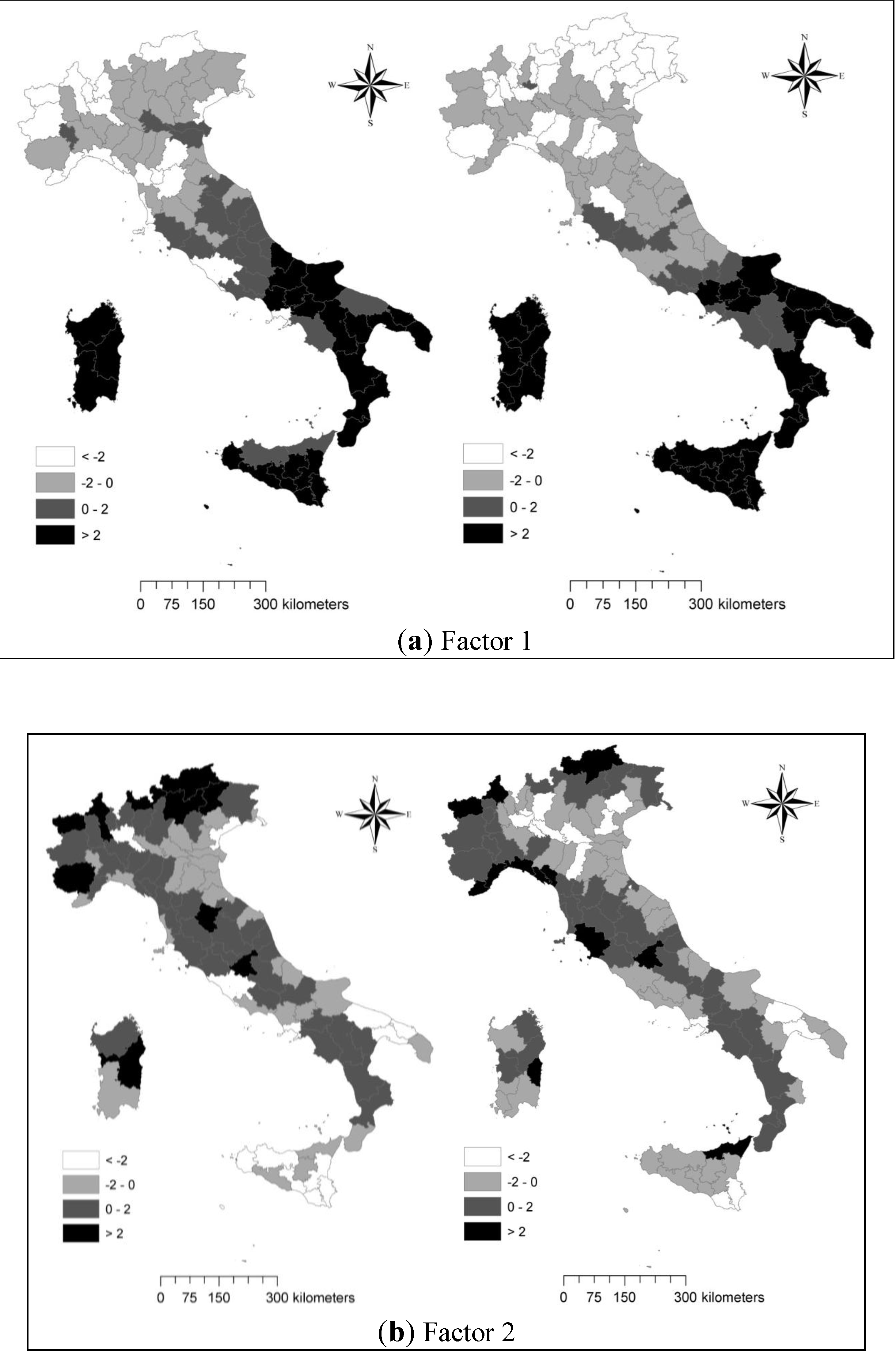
3.3. Principal Components Analysis

Preliminary analysis suggests that PCA can be successfully applied to the original data matrices: both Kaiser-Meyer-Olkin measure of sampling adequacy and Bartlett’s test of sphericity indicate that PCA is appropriate to analyze data for the years investigated. PCA identifies two main components overall explaining nearly 45% of the total variance. Table 4 reports the loading of each indicator (environmental, socioeconomic and supplementary) on the components.
Table 4. Variables’ loadings on the two principal components extracted by PCA by year.
VariableFactor 1Factor 2
196019701980199020002010196019701980199020002010
STRDEP0.810.770.860.700.120.60−0.19−0.170.050.310.450.37
HEAD−0.58−0.48−0.33−0.27−0.17−0.10−0.49−0.54−0.41−0.35−0.100.12
DEN−0.47−0.38−0.23−0.19−0.13−0.160.660.730.710.720.62−0.46
TUR0.770.66−0.41−0.43−0.44−0.310.240.220.380.420.550.55
INDSIZ0.820.750.610.720.730.610.07−0.04−0.33−0.32−0.27−0.45
SERSIZ0.740.690.580.670.730.76−0.36−0.49−0.47−0.45−0.24−0.21
PRODSER0.240.32−0.21−0.580.770.67−0.26−0.18−0.250.14−0.14−0.24
LAND−0.110.01−0.030.11−0.10−0.020.730.750.780.750.63−0.13
SHRIND0.65−0.560.680.620.680.660.250.260.040.12−0.14−0.37
SHRSER−0.24−0.120.390.340.560.55−0.23−0.33−0.01−0.140.120.38
GDPpro0.860.880.940.930.920.860.01−0.040.02−0.12−0.11−0.12
SATavg0.07−0.11−0.26−0.33−0.51−0.340.520.510.520.470.310.10
SATpro0.380.340.250.240.150.290.640.640.720.710.670.38
ELD0.63−0.53−0.580.63−0.58−0.440.200.220.220.120.270.49
HOT0.64−0.50−0.32−0.33−0.27−0.23−0.24−0.32−0.14−0.33−0.22−0.01
BED−0.35−0.020.590.560.620.59−0.27−0.35−0.34−0.36−0.30−0.22
CRE0.700.630.690.710.740.67−0.29−0.32−0.19−0.22−0.11−0.13
ESAI0.580.690.640.630.620.610.64−0.50−0.54−0.54−0.57−0.56
ESAICV0.210.140.050.02−0.05−0.22−0.20−0.130.110.100.080.19
CQI0.620.710.780.800.840.69−0.39−0.33−0.20−0.13−0.15−0.17
VQI0.590.610.080.130.040.51−0.44−0.33−0.52−0.550.65−0.58
MQI0.160.230.200.250.160.040.690.630.80−0.810.850.80
SQI0.230.270.330.280.370.330.170.160.380.400.510.53
LAT *0.750.820.870.880.870.85−0.32−0.25−0.12−0.06−0.080.00
ELE *−0.08−0.10−0.09−0.15−0.11−0.160.580.530.650.650.690.51
ELECV *−0.12−0.14−0.15−0.15−0.15−0.06−0.32−0.33−0.48−0.50−0.50−0.27
SUP *0.270.220.170.130.180.090.320.270.360.340.310.18
DIF *0.360.360.370.350.330.32−0.24−0.21−0.25−0.25−0.26−0.29
LPS *0.060.240.400.640.710.330.02−0.050.17−0.25−0.020.13
AGR *0.850.840.710.700.510.61−0.090.01−0.070.010.070.06
INC *0.860.880.940.930.920.860.01−0.040.02−0.12−0.11−0.12
SAT *0.330.290.230.200.180.160.300.280.380.360.330.09
SAT% *0.510.570.410.440.180.27−0.020.160.270.230.10−0.26
% variance30.827.125.626.727.925.616.816.818.418.717.414.7
Notes: * indicates supplementary variables; bold entries indicate significant variable loadings.
The first component depicts a north-south gradient (LAT) reflecting the socioeconomic disparities between northern and southern Italy in terms of per-capita value added, economic structure, demographic dynamics and tourism specialization. Climate quality and, at least partially, the ESAI correlated with this gradient suggesting that the polarization in affluent and disadvantaged regions was associated with a polarized distribution of sensitive to SD and unaffected land across the country. Along time, the latitude gradient consolidates its importance although few variables showed a change in the loading sign (e.g., STRDEP was turning towards a negative coefficient in 2010) or lower intensity loadings (e.g., the supplementary variable AGR * possibly indicating a reduced intensity of the disparities in rural specialization between northern and southern Italy).
A restricted number of indicators (DEN, LAND, SATpro, ESAI and LUI) correlated with the component 2 depicting the urban-rural gradient in Italy based on population density, agricultural productivity and land-use intensity. This gradient was negatively correlated with the ESAI (indicating that land vulnerability increased with both population density and agricultural productivity). However, the role of these variables into component 2 declined over time: in 2010 the component was primarily a land-use intensity gradient with a moderate correlation to the ESAI. These findings indicate a change in the geography of both socioeconomic and environmental indicators in the last fifty years.
Figure 1 maps, for each Italian province, the scores on component 1 and for both 1960 and 2010. Northern and southern provinces were clustered along component 1. The most stable provinces over time were found in southern Italy, especially in the two main islands (Sardinia and Sicily). The provinces evolving most rapidly concentrated in north-eastern Italy.
Scores on factor 2 identified rural provinces mainly located in the most disadvantaged areas of northern Italy and along the Apennine mountains. The most stable provinces concentrated along the Apennine mountains in both central/northern and southern Italy. Evolving provinces were found especially in the Po plain and in specific areas of central and southern Italy.
Figure 1. PCA score by component and year (left: 1960, right: 2010) in the Italian provinces.
Sustainability 06 03086 g001

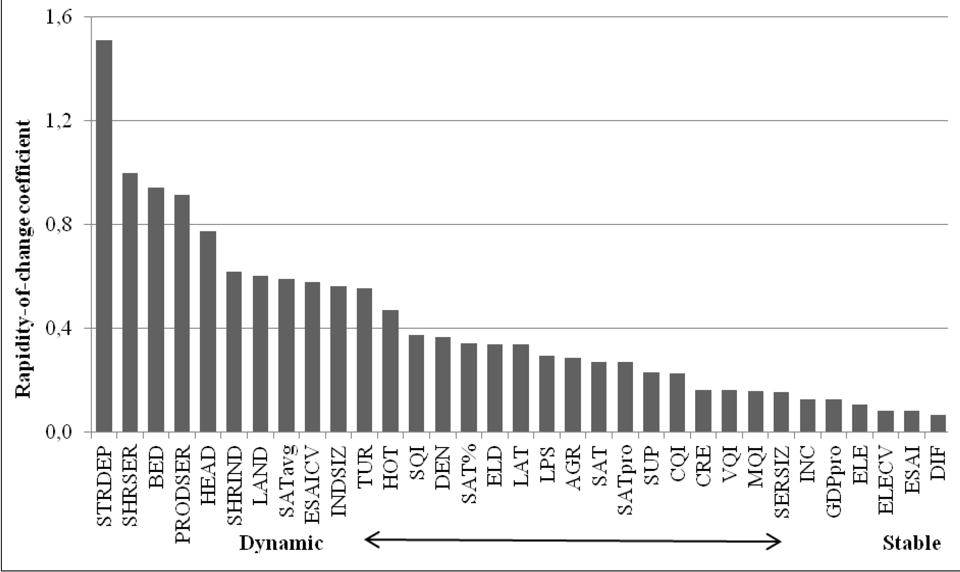
3.4. Assessing “Stable” and “Rapidly Evolving” Variables

Figure 2 ranks the investigated indicators in “dynamic” and “stable” variables according to the rapidity-of-change index based on PCA output. The indicators showing the most rapid changes describe the regional economic structure and indicate a generalized shift towards high-value added and service-oriented local systems based on advanced services, tourism and specific industrial sectors (SHRSER, BED, PRODSER, SHRIND) associated with selected demographic and land-use traits (STRPOP, HEAD, SATavg, LAND). Overall, environmental indicators were classified as relatively “stable” variables together with some socioeconomic and territorial indicators (DIF, GDPpro, INC, SERSIZ, CRE) representing traditional economic gradients in the country.
Figure 2. Indicators ranking according to the rapidity-of-change coefficient.
Sustainability 06 03086 g002
Despite important changes in some economic productivity and competitiveness variables, these results indicate that regional disparities in both socioeconomic (e.g., per-capita value added, population density and the spatial distribution of upper economic functions) and environmental variables (e.g., ESAI) consolidated during the study period mainly because of the impact of local systems poorly evolving from the point of view of the three sustainability pillars (economy- society- environment).

3.5. Canonical Correlation Analysis

In order to achieve a comprehensive description of the relationships existing between socioeconomic and environmental indicators, a canonical correlation analysis was carried out separately for 1960 and 2010 data (Table 5) extracting three relevant factors with a high canonical correlation. In 1960, the first factor (root 1) pointed out the positive relationship between productivity of agricultural land and level of vulnerability to SD. This finding indicates soil vulnerability as a process intrinsically associated with areas characterized by agricultural intensification. Interestingly, in 2010 root 1 identified a wealth gradient in turn associated with population density only. Root 2 identified a wealth gradient characterized by industrial specialization and a dynamic population structure positively associated with climate quality and vegetation quality in 1960. On the contrary, root 2 correlated with all environmental indicators but SQI in 2010 and no significant correlations were observed with socioeconomic indicators. Root 3 accounted for the spatial distribution of specific variables (ESAICV in 1960 and ELD in 2010). Thus, canonical correlation analysis clearly pointed out the changing relationship between the environmental and socioeconomic dimensions during the study period.
Table 5. Results of the canonical correlation analysis applied to the socioeconomic and ecological sets of indicators.
Variable19602010
Root 1Root 2Root 3Root 1Root 2Root 3
STRDEP−0.160.69−0.25−0.20−0.560.29
HEAD−0.21−0.220.03−0.06−0.02−0.01
DEN−0.42−0.52−0.270.740.12−0.15
TUR0.46−0.55−0.120.18−0.55−0.16
INDSIZ0.170.66−0.19−0.42−0.030.37
SERSIZ−0.09−0.450.050.61−0.210.20
PRODSER−0.110.41−0.28−0.49−0.150.04
LAND0.71−0.33−0.27−0.40−0.10−0.17
SHRIND0.240.61−0.27−0.42−0.130.36
SHRSER0.05−0.090.270.320.01−0.36
GDPpro0.040.63−0.130.66−0.370.26
SATavg0.460.33−0.050.03−0.020.49
SATpro0.600.520.030.620.120.12
ELD0.24−0.48−0.010.08−0.400.65
HOT0.01−0.57−0.02−0.35−0.10−0.28
BED−0.06−0.170.130.160.50−0.53
CRE−0.24−0.42−0.03−0.45−0.190.27
ESAI0.700.58−0.060.020.83−0.48
ESAICV−0.380.210.67−0.01−0.290.03
CQI−0.410.79−0.280.380.68−0.19
VQI−0.500.610.310.160.82−0.34
MQI0.780.01−0.42−0.480.740.11
SQI0.260.300.150.46−0.37−0.55
Canonical correlation0.760.720.390.830.580.40
Note: bold entries indicate a correlation coefficient > |0.6|.

4. Discussion

The rapid increase in soil vulnerability to degradation in Europe [28], and especially in Mediterranean Europe, cannot be convincingly explained by the impact of climate changes alone [45]. It also suggests that socioeconomic factors on different spatial scales are important driving forces for SD [46] and multi-dimensional approaches to sustainable development are particularly suited to address this global and, at the same time, local problem [47,48,49,50]. Multidimensional approaches incorporating both time and space dimensions and based on indicators related to the three pillars of sustainability (economy-society-environment) may therefore satisfactory explore long-term latent patterns in the economic structure and jointly describe selected trends in the main factors affecting soil vulnerability [51,52,53,54].
Thus, dynamics of convergence (or divergence) in the level of soil vulnerability to degradation reflect different paths of long-term sustainable (or unsustainable) regional development in the light of specific environmental process. At the same time, variability in the level of soil vulnerability among neighboring areas, possibly reflecting the divide still existing between developed and disadvantaged local systems, pin-points the interaction among socioeconomic pressures and environmental factors. This framework allows to depict differences in the evolution of socioeconomic factors on a local scale, in turn reflecting moderate changes in soil vulnerability spatial patterns [16]. Environmental degradation causing uncertainty in local development paths [55] is becoming a key concept of the knowledge processes which engage to disentangle the interactions among ecological factors, economic performances, socio-cultural dynamics, and political actions [29].
The present study illustrates a multivariate procedure to assess changes in soil vulnerability to degradation in an integrated framework taking into accounts both environmental and socioeconomic aspects. This approach, alternative to the use of composite indexes of sustainable development [16], is rather easy to implement and can be applied to a larger set of indicators when available. Two groups of variables were chosen referring to the economic and ecological aspects of a certain area, but additional themes could be identified according to different interpretations of the SD phenomenon [5,31,53]. The “environmental” dimension derived from the conceptual framework provided by [28], which describes different systems of soil degradation. The socioeconomic dimension is broadly conceived and includes indicators assessing the potential pressures of the economic structure on the environment through variables such as industrial concentration, tourism intensity, agricultural intensification, and population growth [4].
Results of the multivariate exploratory analysis indicate that, over the study period, a complex pattern exists (i) in the soil-landscape dynamics (based on the interactions among the 6 environmental indicators considered), (ii) in the changing socioeconomic structure (based on the interactions among the 17 socioeconomic indicators considered), and (iii) in the relation among the two factors. The development path of Italian local systems revealed unexpected results. Contrary to the widespread belief that in Italy economic performance and environmental quality follow an opposite North-South gradient [56], local systems in marginal areas, characterized by low per-capita income, agricultural specialization and population ageing, seem not to be associated with better and persisting ecological conditions. Instead, local systems in affluent areas, featuring a mix of socioeconomic conditions, the prevalence of the services in the economy and tourism specialization, show only moderate correlations with worse environmental conditions and especially with SD vulnerability (see also [57] for comparable results on the evolution of selected agricultural systems in Northern and Southern Italy). This has some implication for sustainability, because areas with a rapidly changing socio-demographic profile and a dynamic economic structure are compatible with medium-low and stable levels of soil vulnerability. At the same time, socioeconomic local conditions are associated, as pointed out by the results of this study, with various SD processes [23] which can produce worse environmental conditions. Examples of these processes include (i) population growth—urban sprawl—soil sealing, (ii) industrial concentration—soil pollution, (iii) agricultural intensification—soil compaction, (iv) depopulation—land abandonment—soil erosion. The potential role of multi-domain policies within a sustainability strategy is thus evident in the mitigation of SD in southern Europe [18,21,51].

5. Conclusions

The present study have implications of both cognitive (i.e., research) and normative type (i.e., policy support). Addressing in an integrated time and space framework some of the most important aspects of soil vulnerability—taken as an emblematic sustainability process—is an urgent need for both monitoring and policy purposes. In fact, raising issues related with integrated socioeconomic and ecological matters to achieve a reduction in regional disparities and a more sustainable development path represents a meaningful tool for both monitoring strategies and policy implementation in economically-disadvantaged and ecologically fragile regions [58].
Our results confirm that land mismanagement triggered by unsustainable socioeconomic development is emerging as a crucial aspect of soil degradation in already vulnerable areas [13]. However, due to its complexity and multi-dimensionality [59], this concept is rather difficult to define operatively and to monitor in the long-term in a sustainability perspective [60]. Since land is managed for multiple benefits, such as agricultural production, biodiversity conservation, water and soil quality and supporting human life, socioeconomic and environmental targets should be considered jointly in order to ensure long-term sustainability and preventing abuse of land [27]. This study demonstrates that the spatial distribution of SD vulnerability in Italy is reflected into defined socioeconomic contexts on the local scale in turn affecting landscape configuration and structure and negatively influencing sustainable land management policies [61]. This indicates the need of more effective mitigation strategies addressing the specificity of local socioeconomic contexts. The proposed approach proved suitable to identify target variables and local systems for the development of specific sustainable land management strategies.
Future research should improve short-term sustainability scenarios under various assumptions dealing with e.g., climate changes, urbanization, demographic trends, socioeconomic structure, and considering current and past land-uses, the territorial context and short-term ecological/landscape dynamics as the key variables of changes [25,48,62]. The methodology illustrated in this study may contribute to shed lights to such dynamics by providing on objective way to classify local systems and to profile the most typical factors according to their potential of change and to the implications for long-term sustainability.

Acknowledgments

The research described in this paper has been funded in part by Sapienza University of Rome under the DESERT Project. We are grateful to two anonymous referees for their extensive comments, that allow us to substantially improve the quality of the paper.

Author Contributions

Luca Salvati had the original idea for the study. Marco Zitti was responsible for data collecting. Luca Salvati and Marco Zitti carried out the analysis. Margherita Carlucci added critical intellectual content and reviewed plan documents and literature. All the authors drafted the manuscript, and approved the final one.

Conflicts of Interest

The authors declare no conflict of interest.

References and Notes

  1. Briassoulis, H. Governing desertification in Mediterranean Europe: The challenge of environmental policy integration in multi-level governance contexts. Land Degrad. Dev. 2011, 22, 313–325. [Google Scholar] [CrossRef]
  2. Geist, H. The Causes and Progression of Desertification (Ashgate Studies in Environmental Policy and Practice); Ashgate Publishing Limited: Aldershot, UK, 2005. [Google Scholar]
  3. Fernandez, R.J. Do humans create deserts? Trends Ecol. Evol. 2002, 17, 6–7. [Google Scholar] [CrossRef]
  4. Patterson, T.; Gulden, T.; Cousins, K.; Kraev, E. Integrating environmental, social and economic systems: A dynamic model of tourism in Dominica. Ecol. Model. 2004, 175, 121–136. [Google Scholar] [CrossRef]
  5. Huby, M.; Owen, A.; Cinderby, S. Reconciling socio-economic and environmental data in a GIS context: An example from rural England. Appl. Geogr. 2007, 27, 1–13. [Google Scholar] [CrossRef]
  6. Morse, S. On the use of headline indices to link environmental quality and income at the level of the nation state. Appl. Geogr. 2008, 28, 77–95. [Google Scholar] [CrossRef] [Green Version]
  7. Pisani-Ferry, J. What’s wrong with Lisbon? Available online: http://www.scribd.com/doc/55714442/tp-010605-lisbon (accessed on 10 March 2014).
  8. Hudson, R. Region and place: Rethinking regional development in the context of global environmental change. Prog. Hum. Geogr. 2007, 31, 827–836. [Google Scholar] [CrossRef] [Green Version]
  9. Dall’Erba, S.; Percoco, M.; Piras, G. The European regional growth process revisited. Spat. Econ. Anal. 2008, 3, 7–25. [Google Scholar] [CrossRef]
  10. Tumpel-Gugerell, G. Introduction: Welcome remarks from the 2001 Conference. In Economic Convergence and Divergence in Europe: Growth and Regional Development in an Enlarged European Union; Tumpel-Gugerell, G., Mooslechner, P., Eds.; Edward Elgar: Cheltenham, UK, 2003; pp. 1–8. [Google Scholar]
  11. Millennium Ecosystem Assessment. Ecosystems and Human Well-being: Desertification Synthesis; World Resources Institute: Washington, DC, USA, 2005. [Google Scholar]
  12. Helldén, U.; Tottrup, C. Regional desertification: A global synthesis. Global Planet. Change 2008, 64, 169–176. [Google Scholar] [CrossRef]
  13. Bowyer, C.; Withana, S.; Fenn, I.; Bassi, S.; Lewis, M.; Cooper, T.; Benito, P.; Mudgal, S. Land Degradation and Desertification; European Parliament: Bruxelles, Belgium, 2009. [Google Scholar]
  14. Zuindeau, B. Territorial equity and sustainable development. Environ. Values 2007, 16, 253–268. [Google Scholar] [CrossRef]
  15. Van Delden, H.; Luja, P.; Engelen, G. Integration of multi-scale dynamic spatial models of socio-economic and physical processes for river basin management. Environ. Model. Software 2007, 22, 223–238. [Google Scholar] [CrossRef]
  16. Salvati, L.; Zitti, M. Territorial disparities, natural resource distribution, and land degradation: A case study in southern Europe. GeoJournal 2007, 70, 185–194. [Google Scholar] [CrossRef]
  17. Vogt, J.V.; Safriel, U.; Bastin, G.; Zougmore, R.; von Maltitz, G.; Sokona, Y.; Hill, J. Monitoring and Assessment of Land Degradation and Desertification: Towards new conceptual and integrated approaches. Land Degrad. Dev. 2011, 22, 150–165. [Google Scholar] [CrossRef]
  18. Onate, J.J.; Peco, B. Policy impact on desertification: Stakeholders’ perceptions in southeast Spain. Land Use Policy 2005, 22, 103–114. [Google Scholar] [CrossRef]
  19. Pérez-Sirvent, C.E.; Martínez-Sánchez, M.J.; Vidal, J.; Sánchez, A. The role of low quality irrigation water in the desertification of semi-arid zones in Murcia, SE Spain. Geoderma 2003, 113, 109–125. [Google Scholar] [CrossRef]
  20. Portnov, B.A.; Safriel, U.N. Combating desertification in the Negev: Dryland agriculture vs. dryland urbanization. J. Arid. Environ. 2004, 56, 659–680. [Google Scholar] [CrossRef]
  21. Iosifides, T.; Politidis, T. Socio-economic dynamics, local development and desertification in western Lesvos, Greece. Local Environ. 2005, 10, 487–499. [Google Scholar] [CrossRef]
  22. Conacher, A.J.; Sala, M. Land Degradation in Mediterranean Environments of the World; Wiley: Chichester, UK, 1998. [Google Scholar]
  23. Hill, J.; Stellmes, M.; Udelhoven, T.; Roder, A.; Sommer, S. Mediterranean desertification and land degradation: Mapping related land use change syndromes based on satellite observations. Global Planet. Change 2008, 64, 146–157. [Google Scholar] [CrossRef]
  24. Salvati, L.; Bajocco, S.; Mancini, A.; Gemmiti, R.; Carlucci, M. Socioeconomic development and vulnerability to land degradation in Italy. Reg. Environ. Change 2011, 11, 767–777. [Google Scholar] [CrossRef]
  25. Marathianou, M.; Kosmas, K.; Gerontidis, S.; Detsis, V. Land-use evolution and degradation in Lesvos (Greece): An historical approach. Land Degrad. Dev. 2000, 11, 63–73. [Google Scholar]
  26. Costantini, E.A.C.; Urbano, F.; Aramini, G.; Barbetti, R.; Bellino, F.; Bocci, M.; Bonati, G.; Fais, A.; L’Abate, G.; Loj, G.; et al. Rationale and methods for compiling an atlas of desertification in Italy. Land Degrad. Dev. 2009, 20, 261–276. [Google Scholar] [CrossRef]
  27. Máñez Costa, M.A.; Moors, E.J.; Fraser, E.D.G. Socioeconomics, Policy, or Climate Change: What is Driving Vulnerability in Southern Portugal? Ecol. Soc. 2011, 16. Article 28. [Google Scholar]
  28. Montanarella, L. Trends in land degradation in Europe. In Climate and Land Degradation; Sivakumar, M.V., N’diangui, N., Eds.; Springer: Berlin, Germany, 2007; pp. 181–193. [Google Scholar]
  29. Ibanez, J.; Martinez Valderrama, J.; Puigdefabregas, J. Assessing desertification risk using system stability condition analysis. Ecol. Model. 2008, 213, 180–190. [Google Scholar] [CrossRef] [Green Version]
  30. Felice, E. Regional development: Reviewing the Italian mosaic. J. Mod. Ital. Stud. 2010, 15, 64–80. [Google Scholar] [CrossRef]
  31. Siche, J.R.; Agostinho, F.; Ortega, E.; Romeiro, A. Sustainability of nations by indices: Comparative study between environmental sustainability index, ecological footprint and the emergy performance indices. Ecol. Econ. 2008, 66, 628–637. [Google Scholar] [CrossRef]
  32. Karlsson, R. Inverting sustainable development? Rethinking ecology, innovations and spatial limits. Int. J. Environ. Sustain. Dev. 2007, 6, 273–289. [Google Scholar] [CrossRef]
  33. Thornes, J.B. Emerging mosaics. In Mediterranean Desertification: A Mosaic of Processes and Responses; Geeson, N.A., Brandt, C.J., Thornes, J.B., Eds.; Wiley: Chichester, UK, 2002; pp. 419–427. [Google Scholar]
  34. Hein, L. Assessing the costs of land degradation: A case study for the Puentes catchment, southeast Spain. Land Degrad. Dev. 2007, 18, 631–642. [Google Scholar] [CrossRef]
  35. Barbayiannis, N.; Panayotopoulos, K.; Psaltopoulos, D.; Skuras, D. The influence of policy on soil conservation: A case study from Greece. Land Degrad. Dev. 2011, 22, 47–57. [Google Scholar] [CrossRef]
  36. Salvati, L.; Bajocco, S. Land sensitivity to desertification across Italy: Past, present, and future. Appl. Geogr. 2011, 31, 223–231. [Google Scholar] [CrossRef]
  37. Salvati, L. Mediterranean Desertification and the Economic System. Available online: http://ideas.repec.org/p/des/wpaper/20.html (accessed on 10 March 2014).
  38. Basso, F.; Bove, E.; Dumontet, S.; Ferrara, A.; Pisante, M.; Quaranta, G.; Taberner, M. Evaluating environmental sensitivity at the basin scale through the use of geographic information systems and remotely sensed data: An example covering the Agri basin—Southern Italy. Catena 2000, 40, 19–35. [Google Scholar] [CrossRef]
  39. Kosmas, C.; Tsara, M.; Moustakas, N.; Karavitis, C. Identification of indicators for desertification. Ann. Arid Zones 2003, 42, 393–416. [Google Scholar]
  40. Ferrara, A.; Salvati, L.; Sateriano, A.; Nolè, A. Performance evaluation and costs assessment of a key indicator system to monitor desertification vulnerability. Ecol Indic. 2012, 23, 123–129. [Google Scholar] [CrossRef]
  41. Lavado Contador, J.F.; Schnabel, S.; Gomez Gutierrez, A; Pulido Fernandez, M. Mapping sensitivity to land degradation in Extremadura, SW Spain. Land Degrad. Dev. 2009, 20, 129–144. [Google Scholar] [CrossRef]
  42. Salvati, L.; Smiraglia, D.; Bajocco, S.; Ceccarelli, T.; Zitti, M.; Perini, L. Map of Long-Term Changes in Land Sensitivity to Degradation of Italy. J. Maps 2014, 10, 65–72. [Google Scholar] [CrossRef]
  43. Rubio, J.L.; Bochet, E. Desertification indicators as diagnosis criteria for desertification risk assessment in Europe. J. Arid Environ. 1998, 39, 113–120. [Google Scholar] [CrossRef]
  44. Trisorio, A. The Sustainability of Italian Agriculture; Italian National Institute of Agricultural Economics (INEA): Rome, Italy, 2005. [Google Scholar]
  45. Garcia Latorre, J.; Garcia-Latorre, J.; Sanchez-Picon, A. Dealing with aridity: Socio-economic structures and environmental changes in an arid Mediterranean region. Land Use Policy 2001, 18, 53–64. [Google Scholar] [CrossRef]
  46. Abu Hammad, A.; Tumeizi, A. Land degradation: Socioeconomic and environmental causes and consequences in the eastern Mediterranean. Land Degrad. Dev. 2012, 23, 216–226. [Google Scholar] [CrossRef]
  47. Evans, J.; Geerken, R. Discrimination between climate and human-induced dryland degradation. J. Arid. Environ. 2004, 57, 535–554. [Google Scholar] [CrossRef]
  48. Sun, D.F.; Dawson, R.; Li, B.G. Agricultural causes of desertification risk in Minqin, China. J. Environ. Manag. 2006, 79, 348–356. [Google Scholar] [CrossRef]
  49. Wang, X.; Chen, F.; Dong, Z. The relative role of climatic and human factors in desertification in semiarid China. Global Environ. Chang. 2006, 16, 48–57. [Google Scholar] [CrossRef]
  50. Wessels, K.J. Can human-induced land degradation be distinguished from the effects of rainfall variability? A case study in South Africa. J. Arid. Environ. 2007, 68, 271–297. [Google Scholar] [CrossRef]
  51. Kok, K.; Rothman, D.S.; Patel, M. Multi-scale narratives from an IA perspective: Part I. European and Mediterranean scenario development. Futures 2004, 38, 261–284. [Google Scholar]
  52. Yang, X.; Zhang, K.; Jia, B.; Ci, L. Desertification assessment in China: An overview. J. Arid. Environ. 2005, 63, 517–531. [Google Scholar] [CrossRef]
  53. Morse, S.; Vogiatzakis, I.; Griffiths, G. Space and sustainability. Potential for landscape as a spatial unit for assessing sustainability. Sustain. Dev. 2011, 19, 30–48. [Google Scholar] [CrossRef]
  54. Imeson, A. Desertification, Land Degradation and Sustainability; Wiley: Chichester, UK, 2012. [Google Scholar]
  55. Thornes, J.B. Stability and instability in the management of Mediterranean desertification. In Environmental Modelling: Finding Simplicity in Complexity; Wainwright, J., Mulligan, M., Eds.; Wiley: Chichester, UK, 2004; pp. 303–315. [Google Scholar]
  56. Floridi, M.; Pagni, S.; Falorni, S.; Luzzati, T. An exercise in composite indicators construction: Assessing the sustainability of Italian regions. Ecol. Econ. 2011, 70, 1440–1447. [Google Scholar] [CrossRef]
  57. Niedertscheider, M.; Erb, K. Land system change in Italy from 1884 to 2007: Analysing the North-South divergence on the basis of an integrated indicator framework. Available online: http://www.sciencedirect.com/science/article/pii/S0264837714000167 (accessed on 19 March 2014).
  58. Castellani, V.; Sala, S. Sustainability indicators integrating consumption patterns in strategic environmental assessment for urban planning. Sustainability 2013, 5, 3426–3446. [Google Scholar] [CrossRef]
  59. European Environment Agency. Land in Europe: Prices, taxes and use patterns. Available online: http://www.pedz.uni-mannheim.de/daten/edz-bn/gdf/10/EEA_Land%20pricing.pdf (accessed on 15 February 2014).
  60. Dallara, A.; Rizzi, P. Geographic map of sustainability in Italian local systems. Reg. Stud. 2012, 46, 321–337. [Google Scholar] [CrossRef]
  61. Nkonya, E.; Winslow, M.; Reed, M.S.; Mortimore, M.; Mirzabaev, A. Monitoring and assessing the influence of social, economic and policy factors on sustainable land management in drylands. Land Degrad. Dev. 2011, 22, 240–247. [Google Scholar] [CrossRef]
  62. Corbelle-Rico, E.; Crecente-Maseda, R.; Santé-Riveira, I. Multi-scale assessment and spatial modelling of agricultural land abandonment in a European peripheral region: Galicia (Spain), 1956–2004. Land Use Policy 2012, 29, 493–501. [Google Scholar] [CrossRef]

