Energy and Exergy Analyses of a New Combined Cycle for Producing Electricity and Desalinated Water Using Geothermal Energy


Abstract
:1. Introduction
- Kalina cycle system 5 (KSC5) is primarily focused on direct-fired applications.
- Kalina cycle system 6 (KCS6) is intended for use as the bottoming cycle in a combined cycle.
- Kalina cycle system 11 (KSC11) is particularly useful as a low-temperature geothermal-driven power cycle.
- Kalina cycle system 34 (KSC34) is used in low-temperature geothermal power plants.
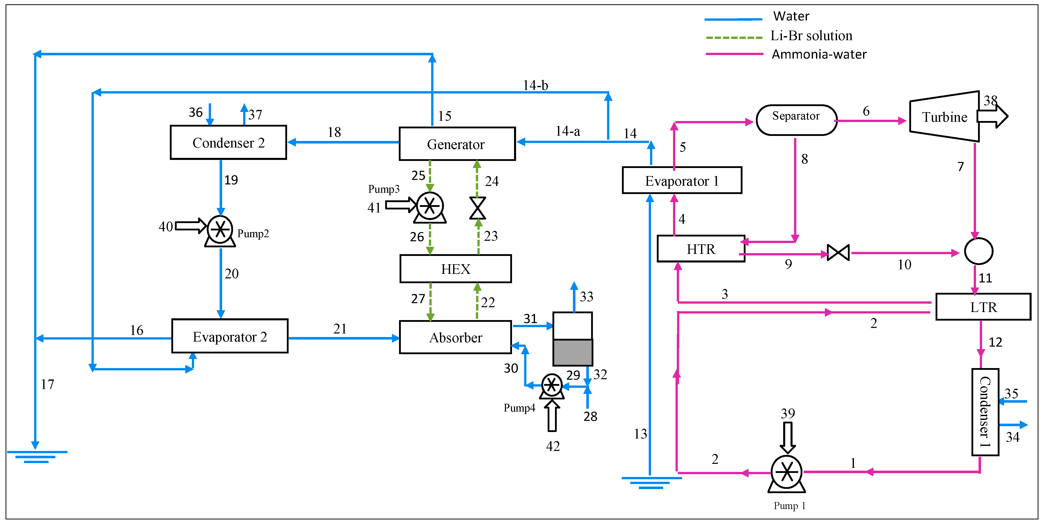
2. System Description
2.1. Kalina Cycle

2.2. LiBr/H2O Absorption Heat Transformer Cycle
2.3. Combined Cycle
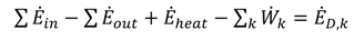
3. Thermodynamic Analysis
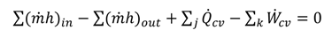
 )in = ∑ (x )out
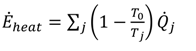
 is the total heat addition rate to the cycle from the heat source, i is the mass flow rate of the fluid, h is the specific enthalpy, ĖD is the rate of exergy destruction, and Ėheat is the net exergy transfer rate associated with heat transfer at temperature T, which is given by:
 [(h − h0) − T0 (s − s0)]
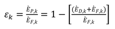
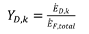
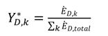
 shows the ratio of component exergy destruction to the total system exergy destruction.
| Subsystem | Exergy relation | Energy relation |
|---|---|---|
| Kalina cycle | ||
| Evaporator 1 | ĖD,eva 1 = T0 [ 4(s5 − s4) + 13(s14 − s13)] | 4(h5 − h4) = 13(h14 − h13) |
| Separator | ĖD,sep = T0 [ 6s6 + 8s8− 5s5] | 5x5 = 6x6 + 8x8 |
| Turbine | ĖD,Tur = T0 [ 6(s6 − s7)] |  |
| LT Recuperator | ĖD,LTR = T0 [ 11(s12 − s11) + 2(s3 − s2)] | 2(h3 − h2) = 11(h12 − h11) |
| HT Recuperator | ĖD,HTR = T0 [ 3(s4 − s3) + 8(s9 − s8)] | 3(h4 − h3)= 8(h9 − h8) |
| Pump 1 | ĖD,P,1= T0 [ 1(s2 − s1)] | Wp,1 = v2(h2 − h1) |
| Condenser 1 | ĖD,con 1 = T0 [ 1(s1 − s12) + 34(s35 − s34)] |  |
| LiBr/H2O cycle | ||
| Evaporator 2 | ĖD,eva 2 = T0 [ 22(s23 − s22) + 15(s15 − s13)] | 13(h13 − h16) = 22(h22 − h23) |
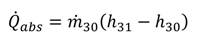
| Absorber | ĖD,Abs = T0 [ 17s17 − 23s23 − 26s26 + 29(s30 − s29)] | 30(h30 − h29) =
17h17 − 23h23 − 26h26 |
| heat exchanger | ĖD,HEX = T0 [ 17(s18 − s17) + 25(s26 − s25)] | 17(h17 − h18) = 25(h25 − h26) |
| Generator | ĖD,Gen = T0 [ 20s20 − 24s24 − 19s19 + 14(s14 − s13)] | 13(h13 − h16) = 19h19 − 20h20 − 24h24 |
| Throttling valve | ĖD,V = T0 [ 24(s25 − s24)] | 18h18 = 19h19 |
| Pump 2 | ĖD,P2 = T0 [ 21(s22 − s21)] | wp,2= v21(h22 − h21) |
| Pump 3 | ĖD,P3 = T0 [ 24(s25 − s24)] | wp,3 = v24(h25 − h24) |
| Pump 4 | ĖD,P4 = T0 [ 2(8s29 − s28)] | wp,4 = v28(h29 − h28) |
| Condenser 2 | ĖD,con 2 = T0 [ 20(s21 − s20) + 35(s36 − s35)] |  |
| Subsystem | Fuel | Product |
|---|---|---|
| Kalina cycle | ||
| Evaporator 1 | Ė13 − Ė14 | Ė5 − Ė4 |
| Turbine | Ė6 − Ė7 | ẆTur |
| LT Recuperator | Ė11 − Ė12 | Ė3 − Ė2 |
| HT Recuperator | Ė8 − Ė9 | Ė4 − Ė3 |
| Pump 1 | Ẇp,1 | Ė2 − Ė1 |
| Condenser 1 | Ė34 − Ė35 | Ė12 − Ė1 |
| LiBr/H2O cycle | ||
| Evaporator 2 | Ė21 − Ė20 | Ė14−b −Ė16 |
| Absorber | Ė31 − Ė30 | (Ė21 + Ė27) − Ė22) |
| heat exchanger | Ė23 − Ė22 | Ė27 − Ė26 |
| Generator | Ė14 − Ė15 | Ė24 − (Ė14 + Ė18) |
| Pump 2 | Ẇp,2 | Ė20 − Ė19 |
| Pump 3 | Ẇp,3 | Ė26 − Ė25 |
| Pump 4 | Ẇp,4 | Ė30 − Ė29 |
| Condenser 2 | Ė36 − Ė37 | Ė18 − Ė19 |
3.1. Assumptions
- (a)
- The geothermal power plants operate at a steady-state condition.
- (b)
- Pressure drops in heat exchangers and pipes are neglected.
- (c)
- The turbines and pumps have non-ideal isentropic efficiencies.
- (d)
- Kinetic and potential energy changes are negligible.
- (e)
- The geofluid is at a saturated liquid condition in the reservoir (x = 0).
- (f)
- Thermodynamic properties of pure water can be used for the geofluid.
- (g)
- Temperature and pressure losses of the geofluid are neglected in the separation and condensation processes.
3.2. Performance Evaluation
 1[(h1 − h17) − T0(s1 − s17)]
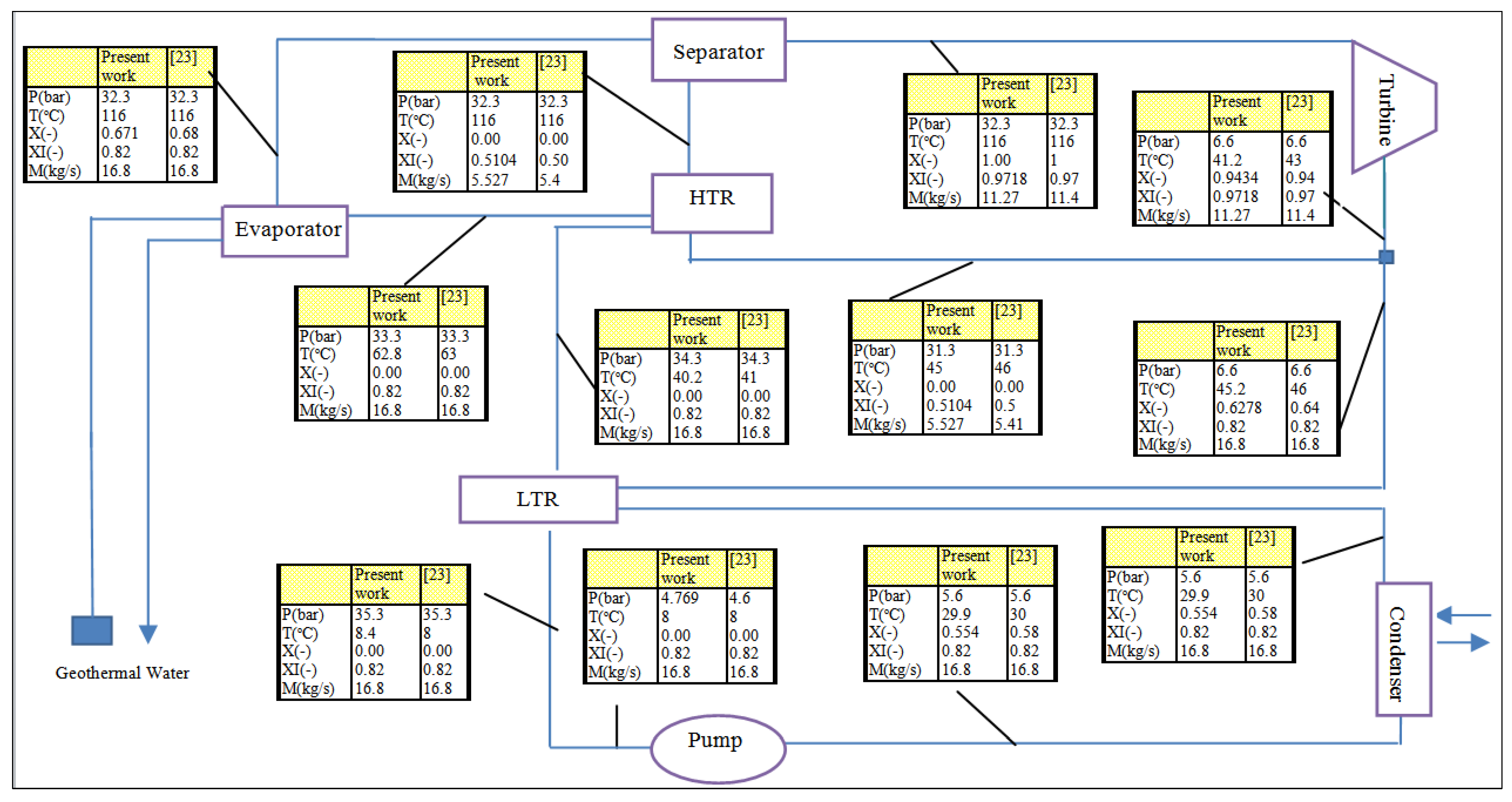
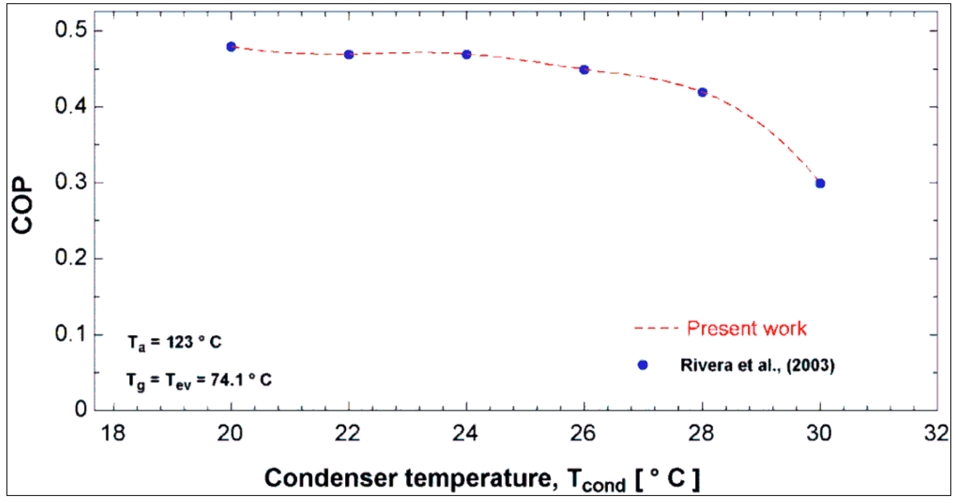
3.3. Model validation
4. Thermoeconomic Analysis
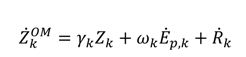
 includes all the other operation and maintenance costs which are independent of investment cost and product exergy. Since the last two terms on the right side of the equation are small compared to the first, these terms may be neglected as is often done [34,35,36].
| Subsystem | Exergy relation | Subsystem | Exergy relation |
|---|---|---|---|
| Kalina cycle | LiBr/H2O cycle | ||
| Evaporator 1 |  | Evaporator 2 |  |
| Separator |  | Generator |  |
| Turbine |  | HEX |  |
| LT Recuperator |  | Absorber |  |
| HT Recuperator |  | Pump 2 | Ċ20 = ŻP,2 + Ċ19 + Ċ40 |
| Pump 1 | Ċ2 = ŻP,1 + Ċ1 + Ċ39 | Pump 3 | Ċ26 = ŻP,3 + Ċ25 + Ċ41 |
| Condenser 1 |  | Pump 4 | Ċ30 = ŻP,4 + Ċ29 + Ċ42 |
| Evaporator 1 |  | Condenser 2 |  |
- A known value is assumed for the unit exergetic cost of the geothermal source (c13 = 1.3) [37].
- The unit exergetic cost of the cooling water is neglected [29], i.e., c33 = 0, c35 = 0 and c27 = 0.
- The auxiliary equations, c14–a = c14–b = c14 and Ċ14 = Ċ14−a + Ċ14−b , are considered for streams 14–a and 14–b.
5. Results and Discussion
| Temperature of the reference environment | 25 °C |
| Pressure of the reference environment | 1 bar |
| Temperature of water from the well | 124 °C |
| Temperature of exit water of evaporator 1 | 80 °C |
| Turbine inlet pressure | 32.3 bar |
| Temperature of water to the well | T14 − 5 |
| Temperature of solution exiting condenser | T0 + 5 |
| Temperature of generator and evaporator 2 | T16 − 3 |
| Mass flow rate of geothermal water | 89 kg/s |
| Temperature of LiBr/H2O solution | 110 °C |
| Mass flow rate of seawater | 12 kg/s |
| Ammonia mass fraction | 82% |
| Turbine isentropic efficiency | 90% |
| Pump isentropic efficiency | 80% |
| Turbine power (kW) | 2452 |
| Condenser 1 heat rejection rate (kW) | 14,172 |
| Pump 1 power (kW) | 80.59 |
| Pump 2 power (kW) | 0.01203 |
| Pump 3 power (kW) | 83.04 |
| Pump 4 power (kW) | 0.1108 |
| Evaporator 1 heat input rate (kW) | 16,543 |
| Evaporator 2 heat input rate (kW) | 1009 |
| Absorber heat transfer rate (kW) | 938.3 |
| Generator heat transfer rate (kW) | 857.3 |
| Condenser 2 heat rejection rate (kW) | 1011 |
| Net power output of Kalina cycle (kW) | 2371 |
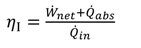
| Net power output and absorber heat rate (kW) | 3226 |
| Heat input rate (kW) | 18,409 |
| Exergy input rate (kW) | 3676 |
| Thermal efficiency (%) | 17.52 |
| Exergy efficiency (%) | 67.38 |
| State | T (°C) | P (bar) | X | (kg/s) | Ė ph (kJ/kg) | Ė ch (kJ/kg K) | Ė (kW) | Ċ ($/h) | c ($/GJ) |
|---|---|---|---|---|---|---|---|---|---|
| 1 | 20 | 7.124 | 0 | 17.82 | 3100 | 289,132 | 292,231 | 2455 | 2.333 |
| 2 | 20.6 | 32.3 | - | 17.82 | 3164 | 289,132 | 292,295 | 2455 | 2.333 |
| 3 | 44.6 | 32.3 | - | 17.82 | 3214 | 289,132 | 292,345 | 2457 | 2.335 |
| 4 | 65.6 | 32.3 | - | 17.82 | 3382 | 289,132 | 292,513 | 2460 | 2.337 |
| 5 | 118 | 32.3 | 0.6824 | 17.82 | 6388 | 289,132 | 295,520 | 2480 | 2.331 |
| 6 | 118 | 32.3 | 1 | 12.16 | 5915 | 233,147 | 239,065 | 2007 | 2.332 |
| 7 | 46.4 | 7.124 | 0.9417 | 12.16 | 3212 | 233,147 | 236,359 | 1984 | 2.332 |
| 8 | 118 | 32.3 | 0 | 5.658 | 470.4 | 55,984 | 56,455 | 475.4 | 2.339 |
| 9 | 49.6 | 32.3 | - | 5.658 | 170.8 | 55,984 | 56,155 | 472.9 | 2.339 |
| 10 | 50 | 7.124 | - | 5.658 | 154.5 | 55,984 | 56,139 | 472.7 | 2.339 |
| 11 | 49.6 | 7.124 | 0.6382 | 17.82 | 3364 | 289,132 | 292,496 | 2457 | 2.333 |
| 12 | 40.4 | 7.124 | 0.5778 | 17.82 | 3228 | 289,132 | 292,359 | 2456 | 2.333 |
| 13 | 124 | 2.25 | - | 89 | 5085 | 0 | 5,085 | 23.8 | 1.3 |
| 14 | 80 | 2.25 | - | 89 | 1689 | 0 | 1,689 | 7.906 | 1.3 |
| 14-a | 80 | 2.25 | - | 40.89 | 913.2 | 0 | 913.2 | 4.274 | 1.3 |
| 14-b | 80 | 2.25 | - | 48.11 | 776 | 0 | 776 | 3.632 | 1.3 |
| 15 | 75 | 2.25 | - | 40.89 | 647.4 | 0 | 647.4 | 3.03 | 1.3 |
| 16 | 75 | 2.25 | - | 48.11 | 761.8 | 0 | 761.8 | 3.565 | 1.3 |
| 17 | 75 | 2.25 | - | 89 | 1409 | 0 | 1409 | 6.595 | 1.3 |
| 18 | 72 | 0.04246 | - | 0.4029 | 18.74 | 0 | 18.74 | 4.012 | 59.48 |
| 19 | 30 | 0.04246 | - | 0.4029 | 0.07032 | 0.07032 | 0.01506 | 59.48 | |
| 20 | 30 | 0.3397 | - | 0.4029 | 0.08235 | 0 | 0.08235 | 0.02232 | 75.29 |
| 21 | 72 | 0.3397 | - | 0.4029 | 134.4 | 0 | 134.4 | 1.224 | 2.529 |
| 22 | 110 | 0.3397 | 0.5511 | 5.034 | 229.5 | 5.643 | 235.2 | 5.979 | 7.063 |
| 23 | 92.73 | 0.3397 | 0.5511 | 5.034 | 193.1 | 5.643 | 198.8 | 5.055 | 7.063 |
| 24 | 64.72 | 0.04246 | 0.5511 | 5.034 | 439.2 | 5.643 | 439.2 | 11.31 | 7.063 |
| 25 | 72 | 0.04246 | 0.5982 | 4.631 | 274.1 | 4.647 | 278.8 | 8.466 | 8.437 |
| 26 | 81.27 | 0.3397 | 0.5982 | 4.631 | 286.8 | 4.647 | 291.5 | 9.307 | 8.87 |
| 27 | 101.4 | 0.3397 | 0.5982 | 4.631 | 319.7 | 4.647 | 324.3 | 10.44 | 8.942 |
| 28 | 25 | 1 | - | 0.365 | 0.03545 | 0 | 0.03545 | 0 | 0 |
| 29 | 98.19 | 0.9494 | - | 15 | 488.1 | 0 | 488.1 | 20.4 | 11.61 |
| 30 | 98.19 | 1.013 | - | 15 | 488.3 | 0 | 488.3 | 20.41 | 11.61 |
| 31 | 100 | 1.013 | - | 15 | 676.6 | 0 | 676.6 | 27.19 | 11.15 |
| 32 | 100 | 1.013 | - | 14.67 | 498.6 | 0 | 498.6 | 20.4 | 11.36 |
| 33 | 100 | 1.013 | - | 0.365 | 178 | 0 | 178 | 8.255 | 12.82 |
| 34 | 15 | 1 | 0 | 677.5 | 485.2 | 0 | 485.2 | 0 | 0 |
| 35 | 20 | 1 | - | 677.5 | 119.6 | 0 | 119.6 | 3.28 | 7.617 |
| 36 | 15 | 1 | - | 48.33 | 34.61 | 0 | 34.61 | 0 | 0 |
| 37 | 20 | 1 | - | 48.33 | 8.532 | 0 | 8.532 | 4.246 | 138.2 |
| 38 | - | - | - | - | - | - | 2452 | 22.74 | 2.257 |
| 39 | - | - | - | - | - | - | 80.59 | 0.7473 | 2.256 |
| 40 | - | - | - | - | - | - | 0.01203 | 0.00011 | 2.576 |
| 41 | - | - | - | - | - | - | 83.04 | 0.7701 | 2.576 |
| 42 | - | - | - | - | - | - | 0.1108 | 0.00102 | 2.576 |
| Subsystem | Ė F ,k (kw) | Ė P ,k (kw) | Ė D ,k (kw) | Z ($) | Ż ($ h−1) | Y D ,k (%) |  | ε k (%) |
|---|---|---|---|---|---|---|---|---|
| Kalina cycle | ||||||||
| Evaporator 1 | 3396 | 3007 | 389 | 94,124 | 2.752 | 4.71 | 24.46 | 88.54 |
| Turbine | 2706 | 2452 | 254 | 494.9 | 0.01447 | 3.06 | 15.97 | 90.61 |
| LTR | 137 | 50 | 87 | 21,735 | 0.6354 | 1.04 | 5.47 | 36.49 |
| HTR | 300 | 168 | 132 | 14,015 | 0.4097 | 1.59 | 0.1 | 56 |
| Separator and valve | 316 | 300 | 16 | 47,663 | 1.393 | 0.19 | 1.006 | 94.93 |
| Pump 1 | 80.59 | 64 | 16.59 | 1806 | 0.05281 | 0.19 | 1.04 | 79.41 |
| Condenser 1 | 364.6 | 128 | 236.6 | 56,327 | 1.647 | 2.85 | 14.88 | 35.1 |
| LiBr/H2O cycle | ||||||||
| Evaporator 2 | 134.31 | 14.2 | 118.31 | 12,594 | 0.3682 | 1.42 | 7.44 | 10.57 |
| Absorber | 223.5 | 188.5 | 35 | 27,998 | 0.8185 | 0.42 | 2.20 | 84.34 |
| HEX | 36.4 | 32.8 | 3.6 | 5327 | 0.1557 | 0.04 | 0.22 | 90.1 |
| Generator | 492.74 | 265.8 | 226.94 | 14,434 | 0.422 | 2.73 | 14.27 | 53.94 |
| Pump 2 | 0.01204 | 0.01203 | 0.0001 | 182.8 | 0.05322 | - | - | - |
| Pump 3 | 83.04 | 12.7 | 70.34 | 1821 | 0.005345 | 0.84 | 4.42 | 15.3 |
| Pump 4 | 0.1108 | 0.11 | 0.0008 | 325.7 | 0.009521 | - | - | - |
| Condenser 2 | 26.078 | 18.66 | 4.418 | 6,344 | 0.1855 | 0.05 | 0.27 | 71.55 |
| Overall system | 8296.4 | 6701.8 | 1589.8 | 305,191.4 | 8.922366 | 19.16 | 100 | 80.77 |


6. Conclusions
- The proposed cycle, which is a combination of Kalina cycle with an ammonia–water working fluid and a heat transformer cycle with lithium bromide–water working fluid, can beneficially replace conventional geothermal power plants. The production of pure water by the proposed cycleis another advantage for the proposed cycle. The first and second law efficiencies of the proposed cycle are around 24% and 13% higher than the corresponding values for the Kalina cycle.
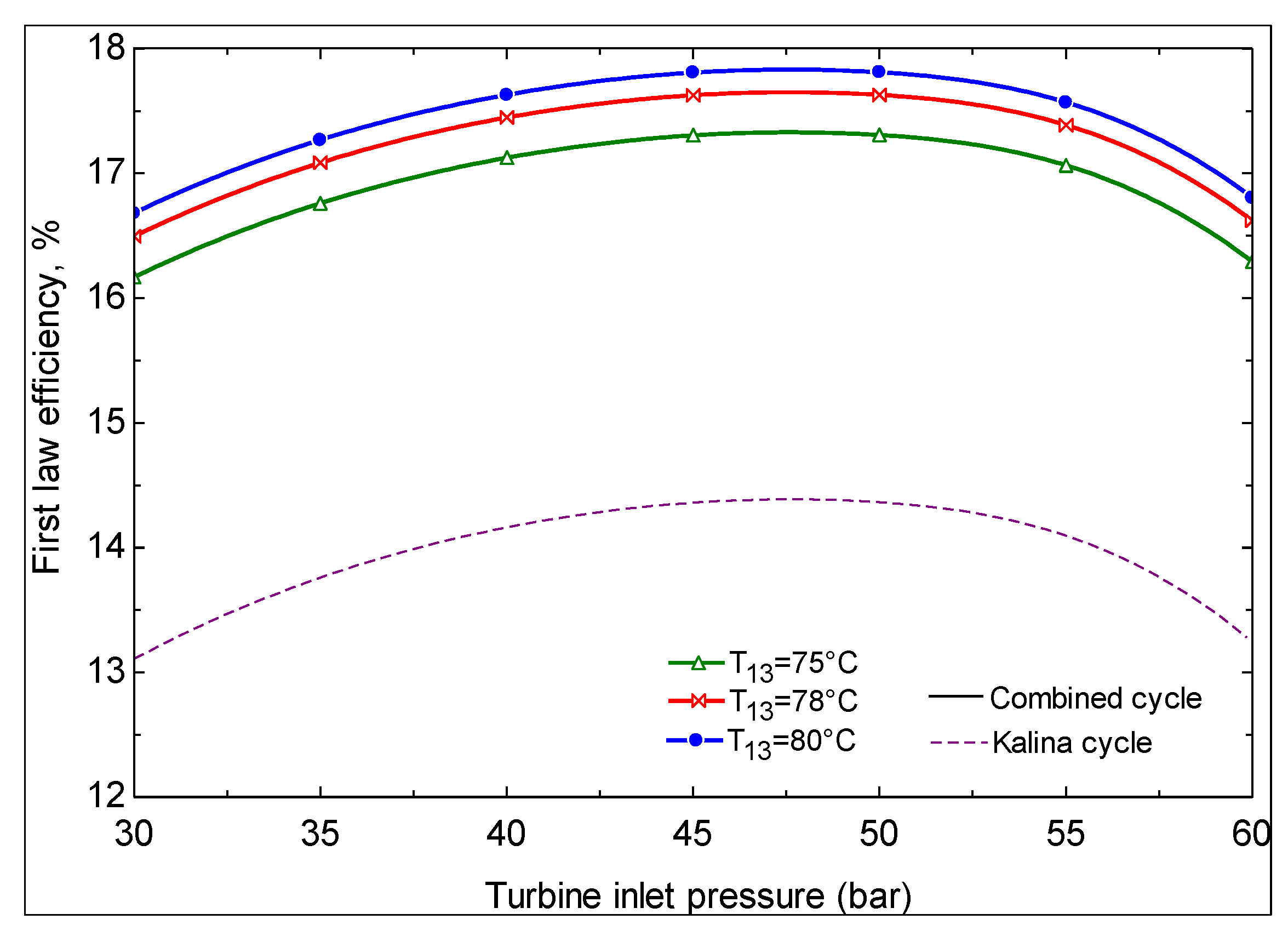
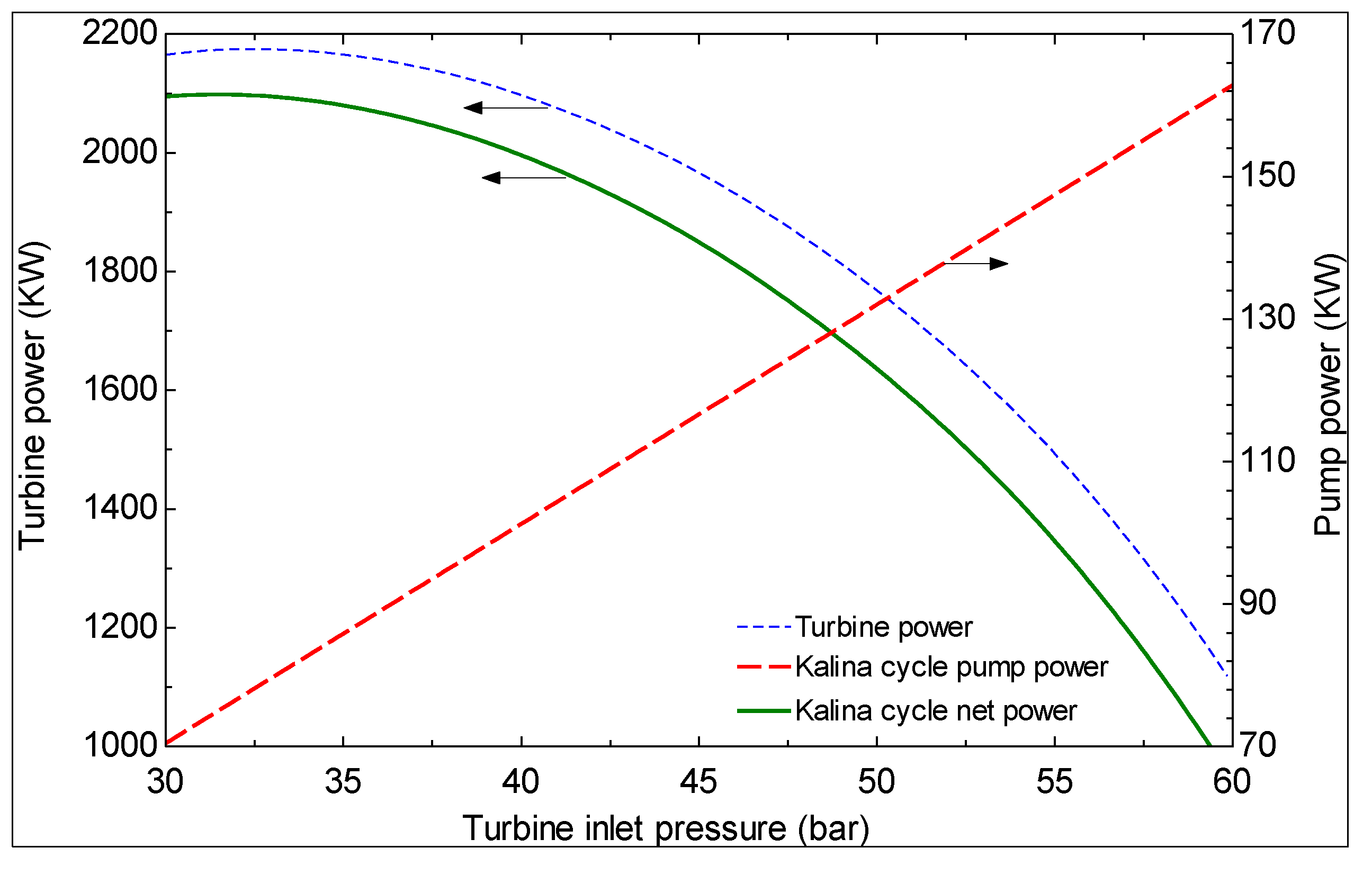
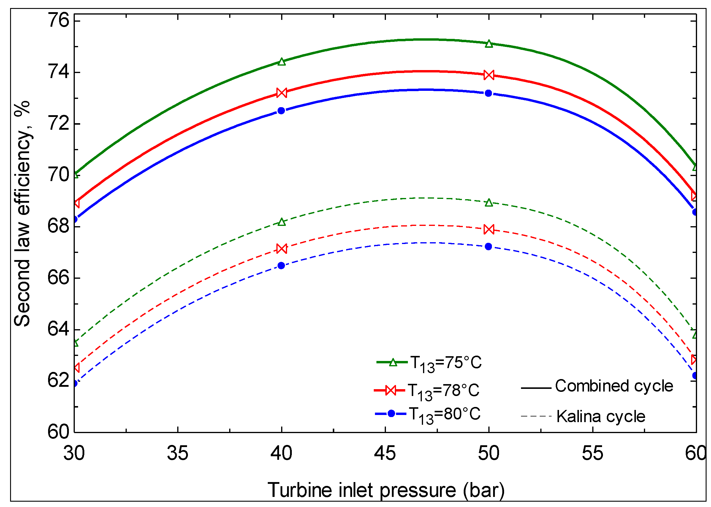
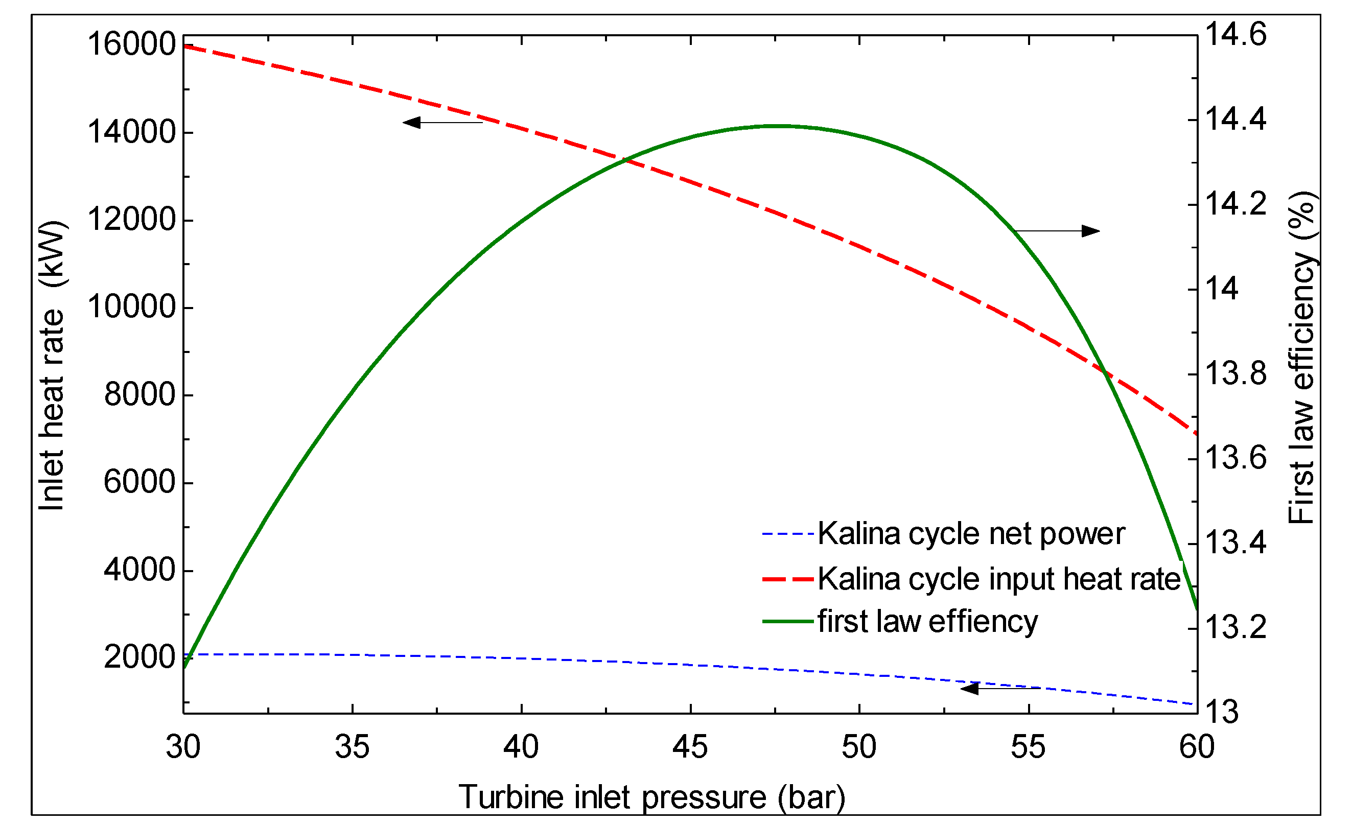
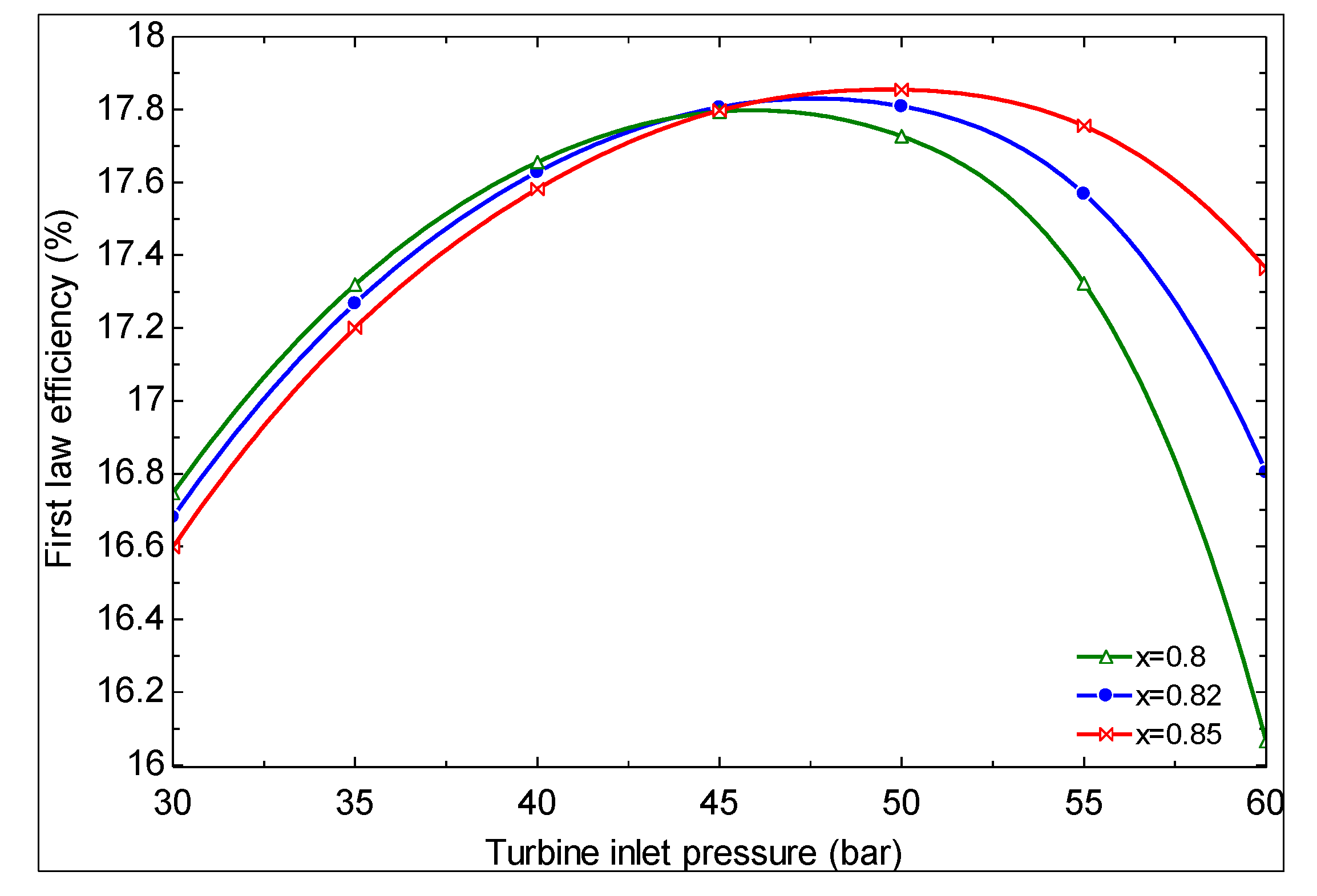
- The first and second law efficiencies are maximized at particular values of turbine inlet pressure. The maximum values increase with increasing ammonia concentration at the evaporator 1 outlet and increasing turbine inlet pressure.
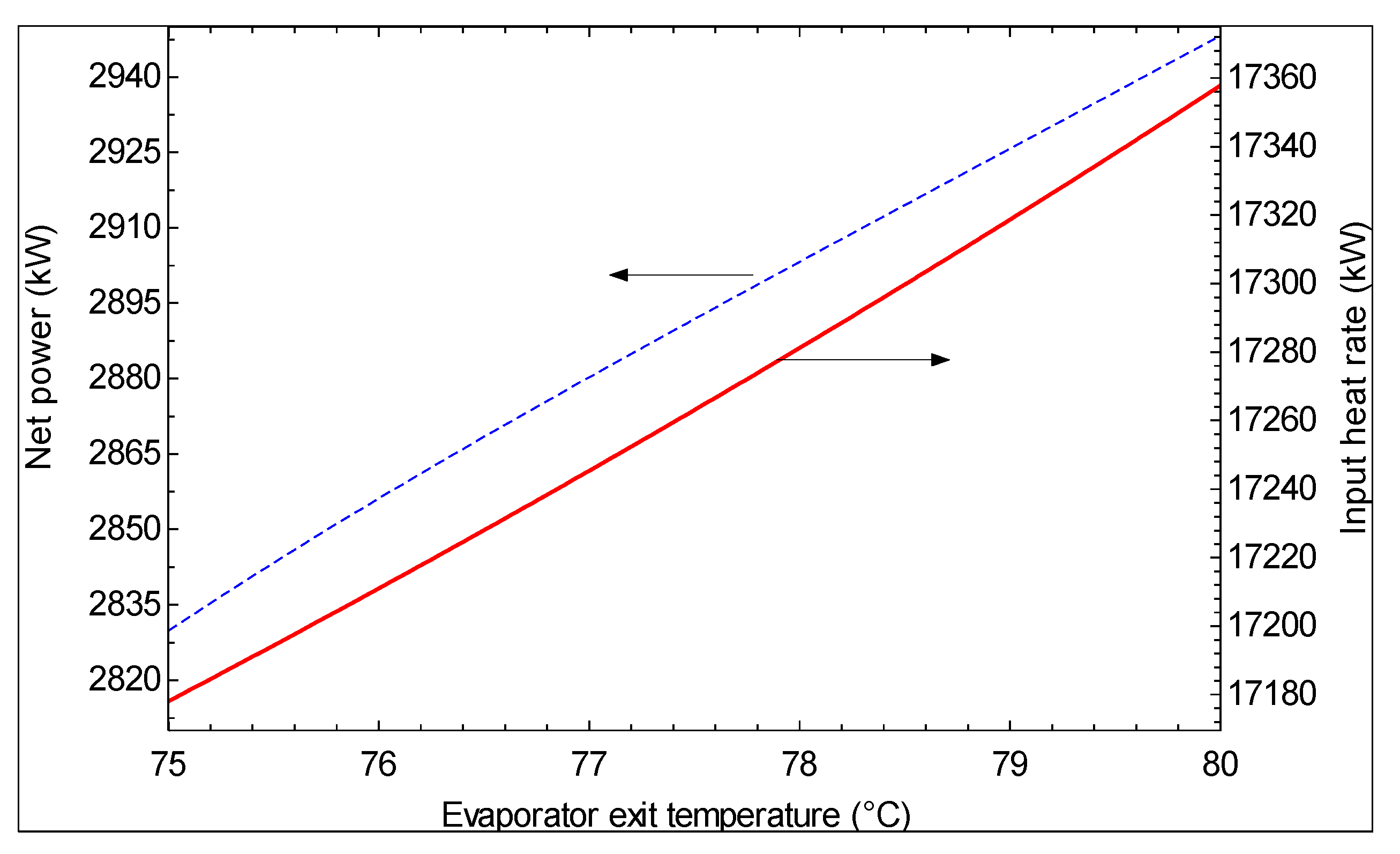
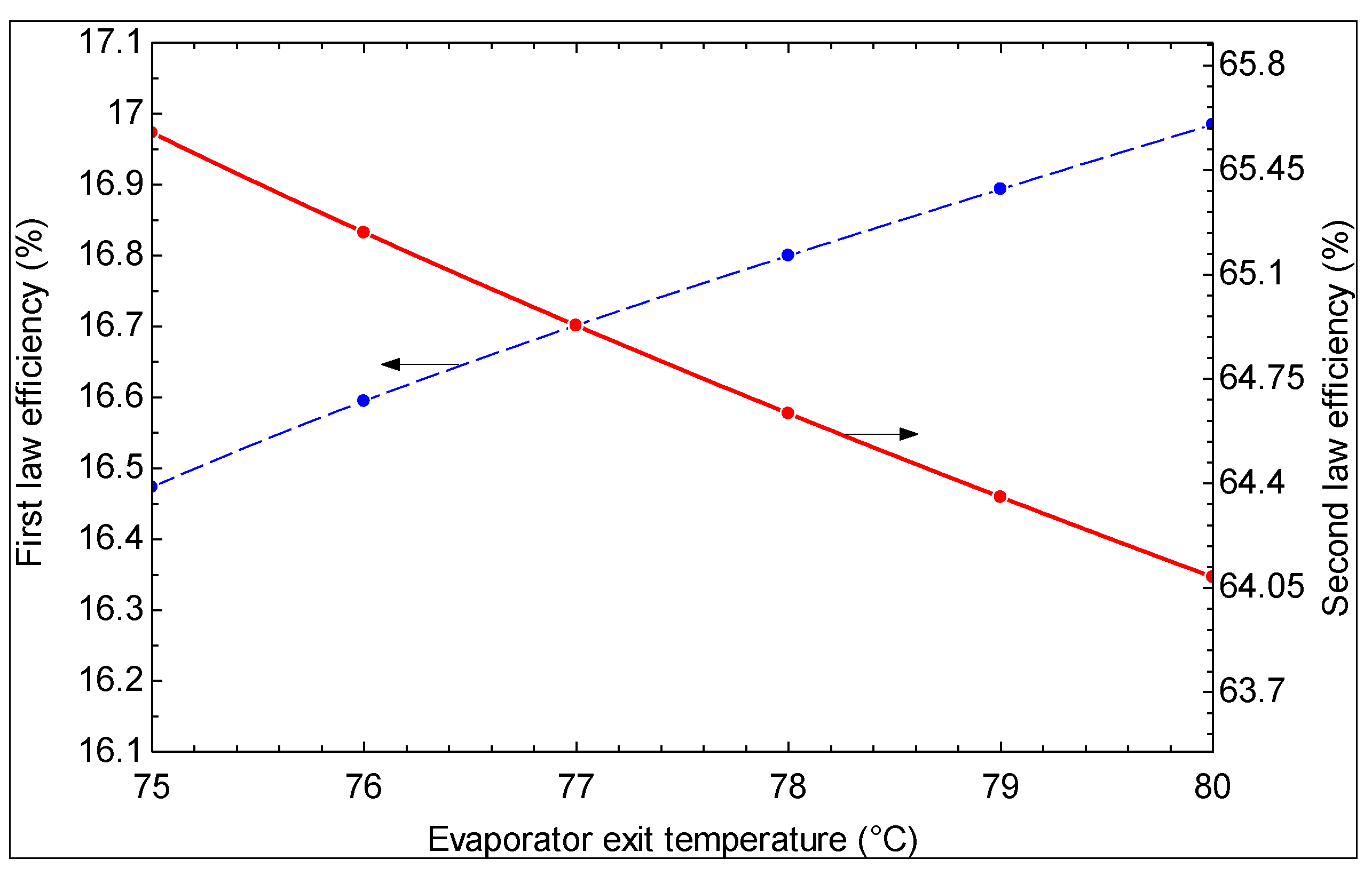
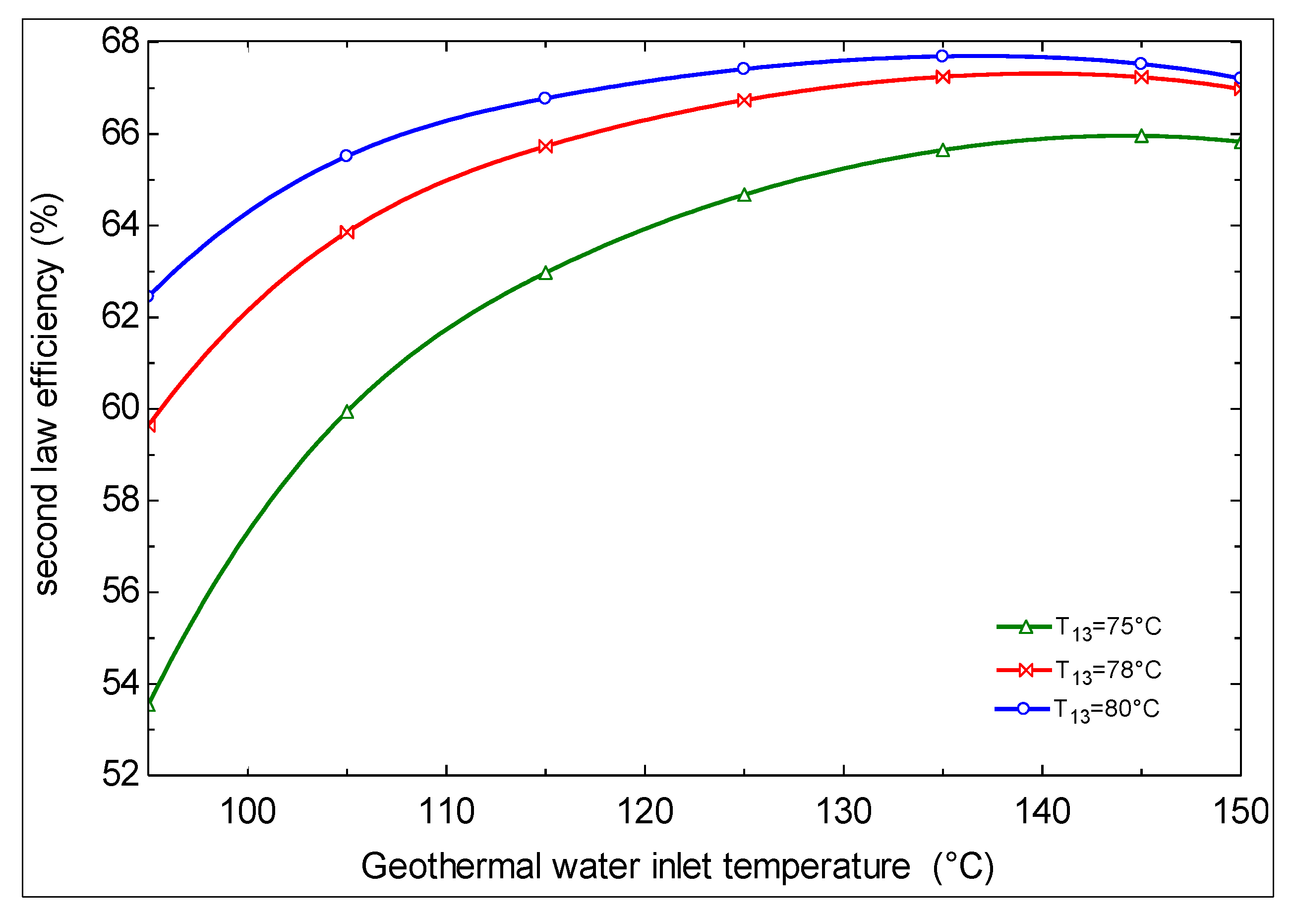
- As the hot water temperature at the outlet of evaporator 1 increases, the first law efficiency increases and the second law efficiency decreases. However, a higher temperature is suggested for the hot water exiting evaporator 1 based on the second law efficiency, which is a more meaningful criterion.
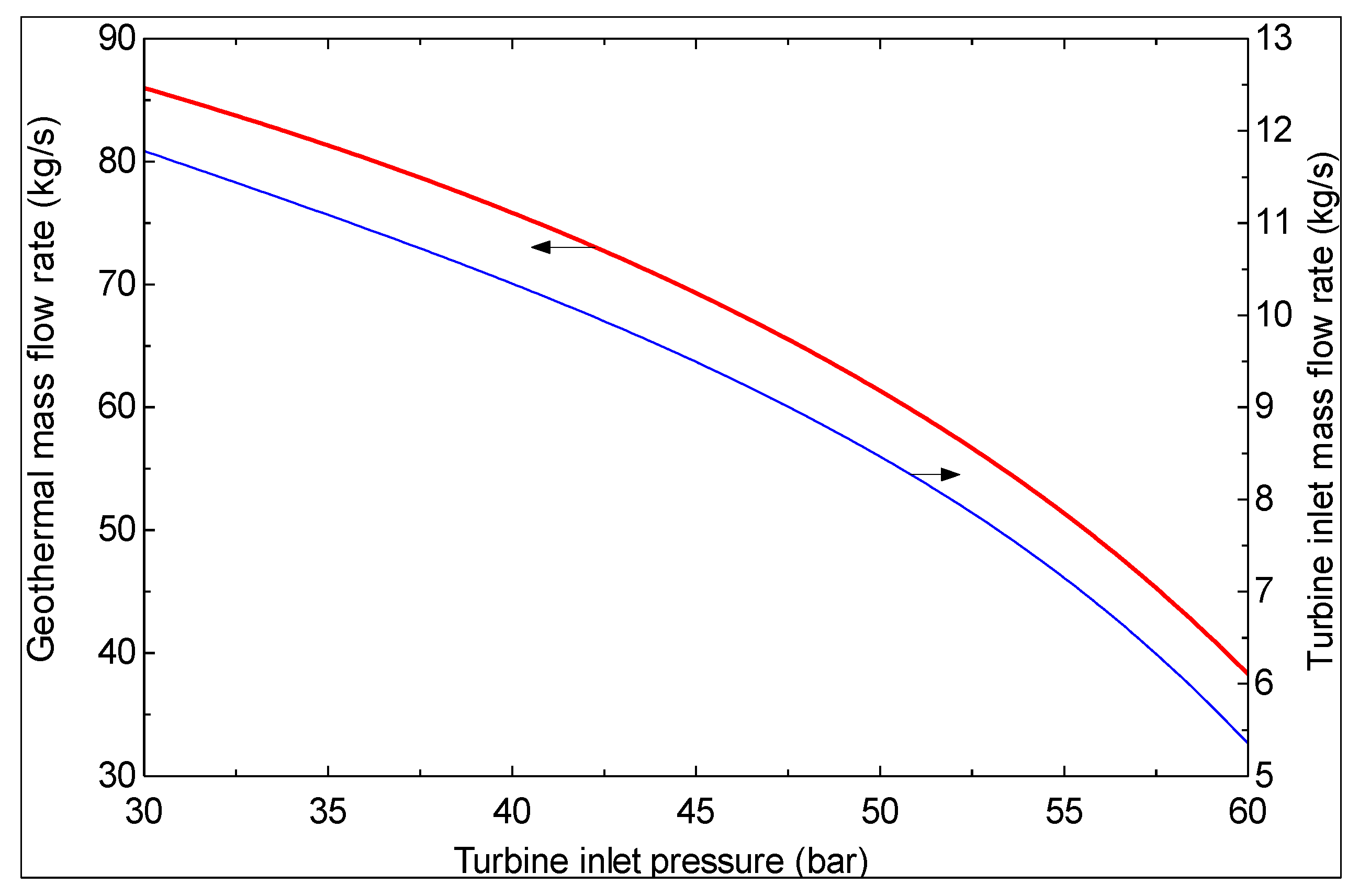
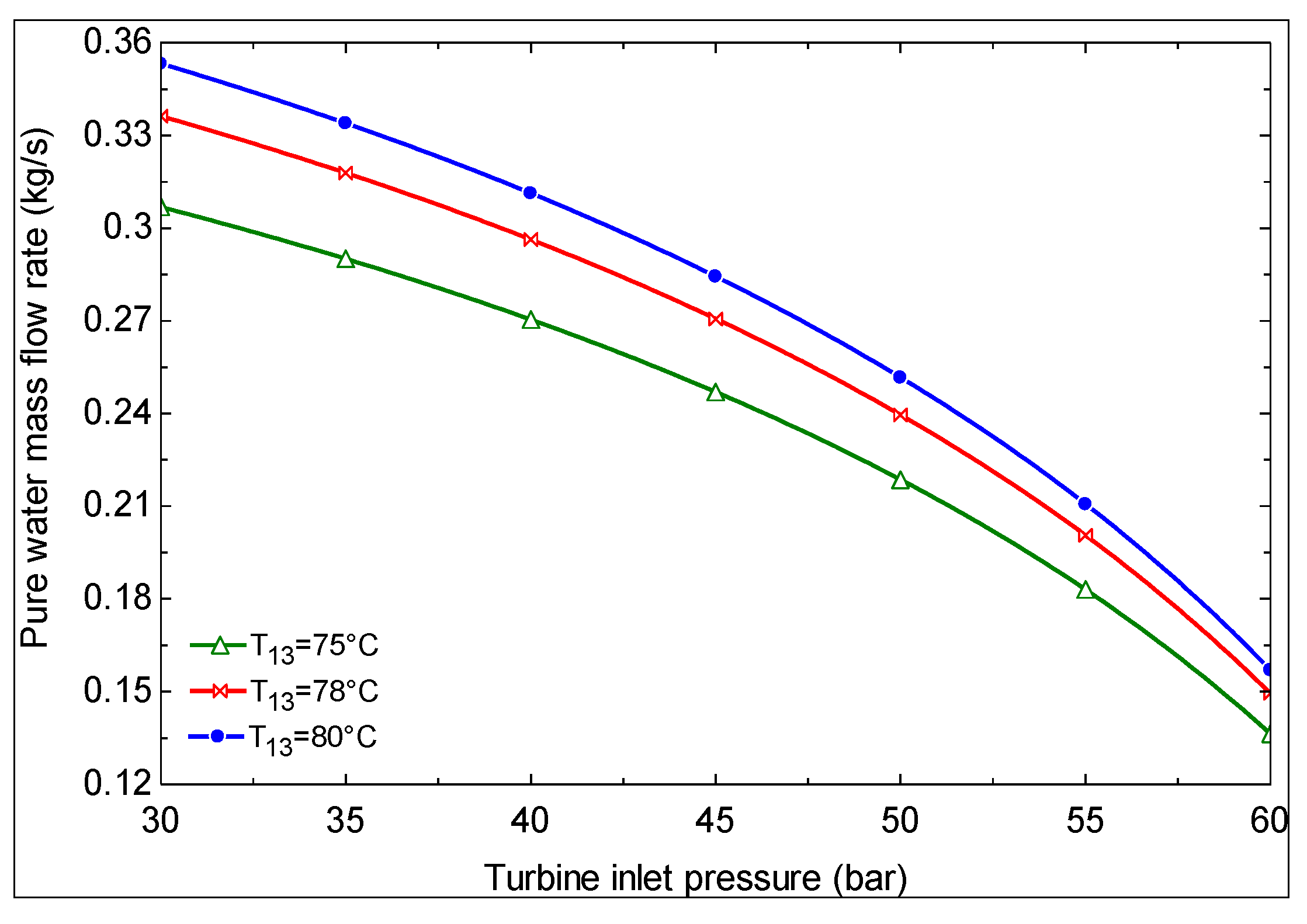
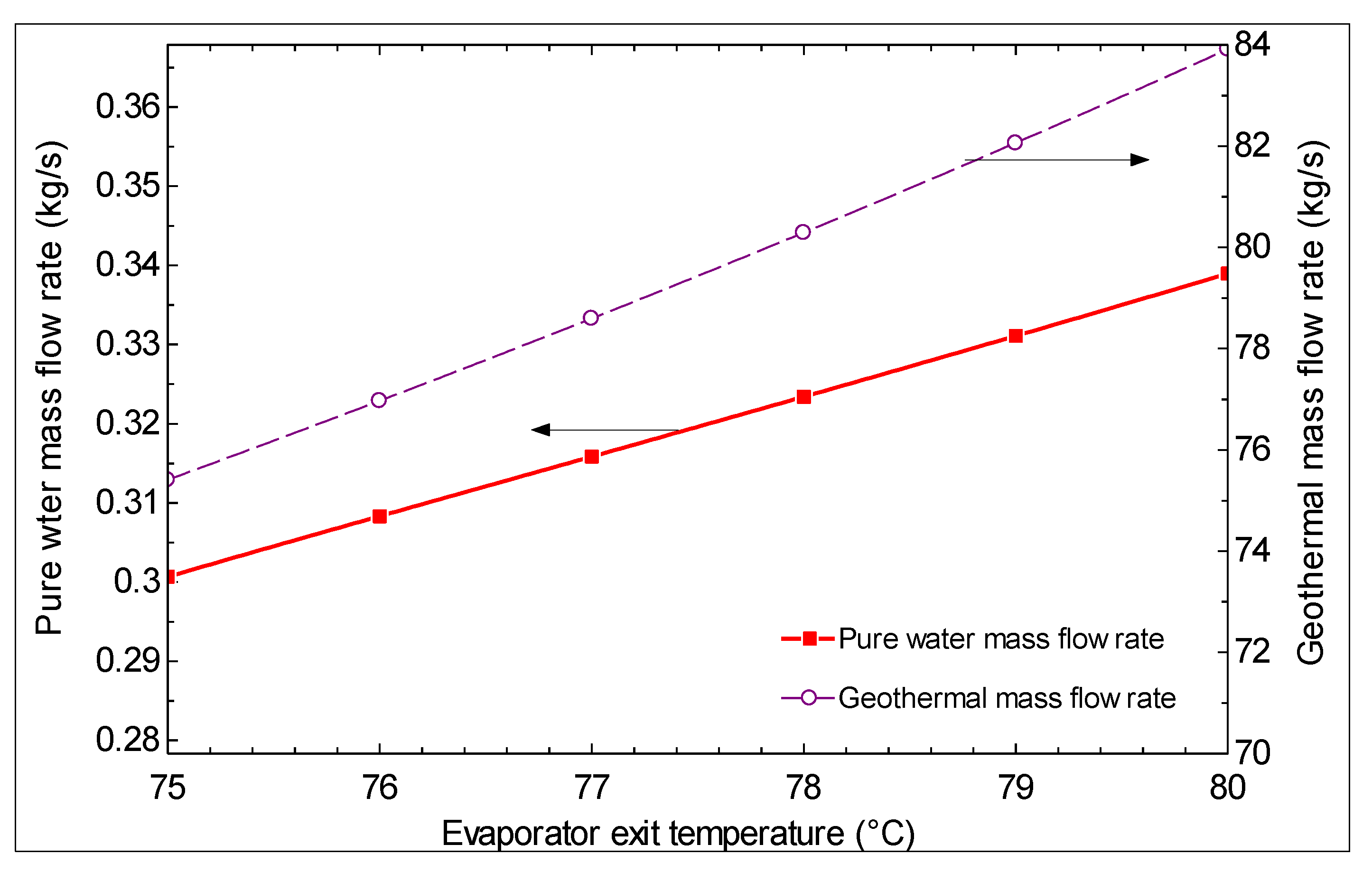
- As the turbine inlet pressure increases and/or the hot water temperature at the exit of evaporator 1 decreases, the produced mass flow rate of pure water decreases.
- Evaporator 1 makes the highest contribution to the cycle exergy destruction, suggesting that more attention may be merited in the design of this component.
- Geothermal water temperatures of less than 124 °C are not convenient for power production with the Kalina cycle. At temperatures above this value, depending on the Kalina cycle conditions, there exists a geothermal water temperature at which the second law efficiency is maximized.
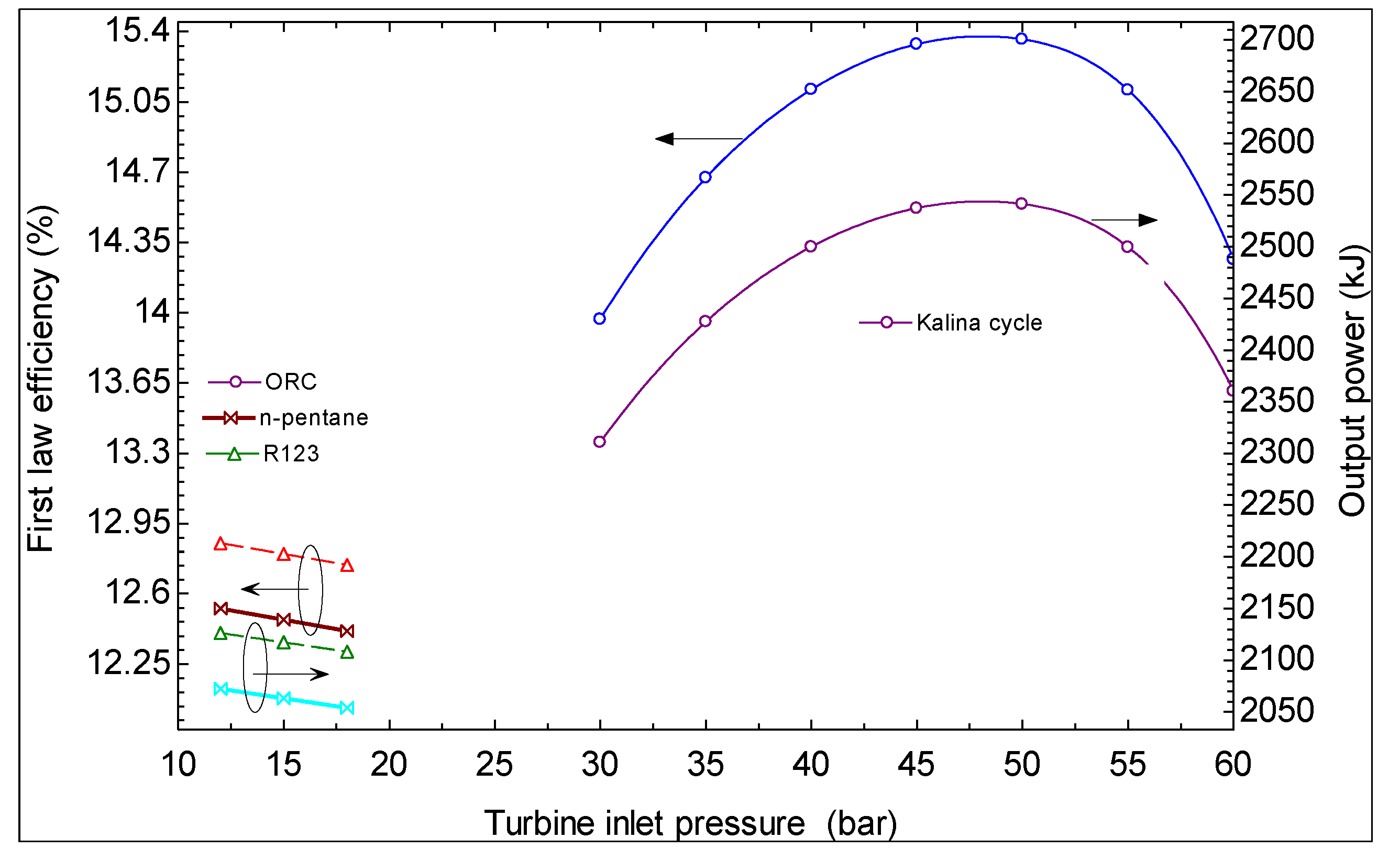
- It is found that using Kalina cycle instead of an ORC to produce power from geothermal energy is advantageous from the viewpoint of thermodynamics.
Nomenclature:
| c | Cost per exergy unit |
| Ċ | Cost rate |
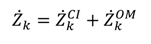
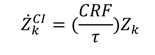
| CI | Capital investment |
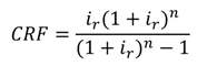
| CRF | Capital recovery factor |
| D | Destruction |
| Ė | Exergy rate |
| e | Specific exergy |
| Ėph | Physical exergy rate |
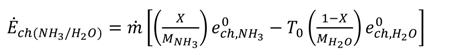
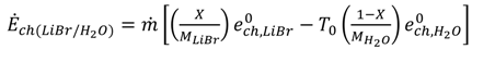
| Ėch | Chemical exergy rate |
 | Dead-state chemical exergy |
| h | Specific enthalpy |
| ir | Interest rate |
| M | Molecular mass |
| | Mass flow rate |
| OM | Operation and maintenance |
| P | Pressure |
 | Heat rate |
| s | Specific entropy |
| | Other operation and maintenance costs |
| T | Temperature |
| T0 | Dead-state temperature |
| v | Specific volume |
| Ẇ | Power output |
| X | Concentration |
| Z | Investment cost of components |
| Ż | Investment cost rate of components |
| τ | Annual plant operation hours |
| γk | Fixed operation and maintenance costs |
| ωk | Variable operation and maintenance costs |
Acknowledgments
Author Contributions
Conflicts of Interest
References
- Shi, X.; Che, D. A combined powesr cycle utilizing low-temperature waste heat and LNG cold energy. Energy Convers. Manag. 2009, 50, 567–575. [Google Scholar] [CrossRef]
- Vidal, A.; Best, R.; Rivero, J.; Cervantes, J. Analysis of a combined power and refrigeration cycle by the exergy method. Energy 2006, 31, 3401–3414. [Google Scholar] [CrossRef]
- Padilla, R.V.; Demirkaya, G.; Goswami, D.Y.; Stefanakos, E.; Rahman, M.M. Analysis of power and cooling cogeneration using ammonia-water mixture. Energy 2010, 35, 4649–4657. [Google Scholar] [CrossRef]
- Wang, J.; Dai, Y.; Zhang, T.; Ma, S. Parametric analysis for a new combined power and ejector-absorption refrigeration cycle. Energy 2009, 34, 1587–1593. [Google Scholar]
- Wang, J.; Dai, Y.; Gao, L. Parametric analysis and optimization for a combined power and refrigeration cycle. Appl. Energy 2008, 113, 135–146. [Google Scholar]
- Tamm, G.; Goswami, D.Y.; Lu, S.; Hasan, A.A. Theoretical and experimental investigation of an ammonia-water power and refrigeration thermodynamic cycle. Solar Energy 2004, 76, 217–228. [Google Scholar] [CrossRef]
- Zamfirescu, C.; Dincer, I. Thermodynamic analysis of a novel ammonia-water trilateral Rankine cycle. Thermochim. Acta 2008, 477, 7–15. [Google Scholar] [CrossRef]
- Maloney, J.D.; Robertson, R.C. Thermodynamic Study of Ammonia-Water Heat Power Cycles; Report CF-53-8-43; Oak Ridge National Laboratory: Oak Ridge, TN, USA, 1953. [Google Scholar]
- Ibrahim, O.M.; Kleins, S.A. Absorption power cycle. Energy 1996, 21, 21–27. [Google Scholar] [CrossRef]
- Kalina, A. Combined Cycle Waste Heat Recovery Power Systems Based on a Novel Thermodynamic Energy Cycle Utilizing Low-Temperature Heat for Power Generation. In Proceeding of the ASME Joint Power Generation Conference, Indianapolis, IN, USA, 25 September 1983; Paper 83-JPGC-GT-3. Available online: http://www.aidic.it/cet/13/35/037.pdf (accessed on 1 January 2014).
- Kalina, A. Combined cycle system with novel bottoming cycle. J. Eng. Gas Turbines Power 1984, 106, 737–742. [Google Scholar] [CrossRef]
- Kalina, A.; Leibowitz, H.M. Application of the Kalina technology to geothermal power generation. Trans. Geoth. Resour. Counc. 1989, 13, 605–611. [Google Scholar]
- El-Sayed, Y.M.; Tribus, M.A. A theoretical comparison of the Rankine and Kalina cycles. Am. Soc. Mech. Eng. 1985, 1, 97–102. Available online: http://www.uran.donetsk.ua/~masters/2006/eltf/bosov/library/kalina.pdf (accessed on 1 January 2014). [Google Scholar]
- Stecco, S.S.; Desideri, U. Thermodynamic Analysis of the Kalina Cycles: Comparisons, Problems, Perspectives. ASME Paper 89-GT-149. In Proceedings of the 34th ASME International Gas Turbine and Aeroengine Congress and Exposition, Toronto, ON, Canada, 4–8 June 1989.
- Martson, C.H. Parametric analysis of the Kalina cycle. J. Eng. Gas Turbine Power 1990, 112, 107–116. [Google Scholar] [CrossRef]
- Desideri, U.; Bidini, G. Study of possible optimization criteria for geothermal power plants. Energy Convers. Manag. 1997, 38, 1681–1691. [Google Scholar] [CrossRef]
- Dejfors, C.; Thorin, E.; Svedberg, G. Ammonia-water power cycles for direct-fired cogeneration applications. Energy Convers. Manag. 1998, 39, 1675–1681. [Google Scholar] [CrossRef]
- Jones, D.A. A Study of the Kalina Cycle System 11 for the Recovery of Industrial Waste Heat with Heat Pump Augmentation. Ph.D. Thesis, Auburn University, Auburn, Alabama, 2011. [Google Scholar]
- Madhawa, H.D.; Golubovic, M.; Worek, W.; Ikegami, Y. The performance of the Kalina cycle system (KSC-11) with low-temperature heat sources. J. Energy Resour. Technol. 2007, 129, 243–247. [Google Scholar] [CrossRef]
- Lolos, P.A.; Rogdakis, E.D. A Kalina power cycle driven by renewable energy sources. Energy 2009, 34, 457–464. [Google Scholar] [CrossRef]
- Bombarda, P.; Invernizzi, C.M.; Pietra, C. Heat recovery from diesel engine: A thermodynamic comparison between Kalina and ORC cycles. Appl. Therm. Eng. 2010, 30, 212–219. [Google Scholar] [CrossRef]
- Arslan, O. Exergoeconomic evaluation of electricity generation by the medium temperature geothermal resources, using a Kalina cycle: Simav case study. Int. J. Therm. Sci. 2010, 49, 1866–1873. [Google Scholar] [CrossRef]
- Ogriseck, S. Integration of Kalina cycle in a combined heat and power plant, a case study. Appl. Therm. Eng. 2009, 29, 2843–2848. [Google Scholar] [CrossRef]
- Sekar, S.; Saravanan, R. Experimental studies on absorption heat transformer coupled distillation system. Desalination 2011, 274, 292–301. [Google Scholar] [CrossRef]
- Rivera, W.; Siqueiros, J.; Martínez, H.; Huicochea, A. Exergy analysis of a heat transformer for water purification increasing heat source temperature. Appl. Therm. Eng. 2010, 30, 2088–2095. [Google Scholar] [CrossRef]
- Rivera, W.; Huicochea, A.; Martínez, H.; Siqueiros, J.; Juárez, D.; Cadenas, E. Exergy analysis of an experimental heat transformer for water purification. Energy 2011, 36, 320–327. [Google Scholar]
- Gomri, R. Energy and exergy analyses of seawater desalination system integrated in a solar heat transformer. Desalination 2009, 249, 188–196. [Google Scholar] [CrossRef]
- Gomri, R. Thermal seawater desalination: Possibilities of using single effect and double effect absorption heat transformer systems. Desalination 2010, 253, 112–118. [Google Scholar] [CrossRef]
- Rivera, W.; Cerezo, J.; Rivero, R.; Cervantes, J.; Best, R. Single stage and double absorption heat transformers used to recover energy in a distillation column of butane and pentane. Int. J. Energy Res. 2003, 27, 1279–1292. [Google Scholar] [CrossRef]
- Klein, S.A.; Alvarda, F.R. Engineering Equation Solver (EES); F-Chart Software: Madison, WI, USA, 2007. [Google Scholar]
- Yari, M. Exergetic analysis of various types of geothermal power plants. Renew. Energy 2010, 35, 112–121. [Google Scholar] [CrossRef]
- Nag, P.K.; Gupta, V.S.K.S. Exergy analysis of the Kalina cycle. Appl. Therm. Eng. 1998, 18, 427–439. [Google Scholar] [CrossRef]
- DiPippo, R. Second Law assessment of binary plants generating power from low-temperature geothermal fluids. Geothermics 2004, 23, 565–586. [Google Scholar] [CrossRef]
- Bejan, A.; Tsatsaronis, G.; Moran, M. Thermal Design and, Optimization; Wiley: New York, NY, USA, 1996. [Google Scholar]
- Misra, R.D.; Sahoo, P.K.; Gupta, A. Thermoeconomic evaluation and optimization of an aqua-ammonia vapour-absorption refrigeration system. Int. J. Refrig. 2006, 29, 47–59. [Google Scholar] [CrossRef]
- Rossa, J.A.; Bazzo, E. Thermodynamic modeling of an ammonia-water absorption system associated with a microturbine. Int. J. Thermodyn. 2009, 12, 38–43. [Google Scholar]
- Dorj, P. Thermoeconomic Analysis of a New Geothermal Utilization CHP Plant in Tsetserleg, Mongoloa. Master Thesis, University of Iceland, Reykjavík, Iceland, 2005. [Google Scholar]
- Misra, R.D.; Sahoo, P.K.; Sahoo, S.; Gupta, A. Thermoeconomic optimization of a single effect water/LiBr vapour absorption refrigeration system. Int. J. Refrig. 2003, 26, 158–169. [Google Scholar] [CrossRef]
- Zare, V.; Mahmoudi, S.M.S.; Yari, M.; Amidpour, M. Thermoeconomic analysis and optimization of an ammonia-water power/cooling cogeneration cycle. Energy 2012, 47, 271–283. [Google Scholar] [CrossRef]
Appendix A

| Component | Reference cost ($) [38] |
|---|---|
| Evaporator | 16,000 |
| Recuperator, heat exchanger | 12,000 |
| Separator | 16,500 |
| Condenser | 8000 |
| Generator | 17,500 |
| Absorber | 16,500 |
| pump | 2100 |
© 2014 by the authors; licensee MDPI, Basel, Switzerland. This article is an open access article distributed under the terms and conditions of the Creative Commons Attribution license (http://creativecommons.org/licenses/by/3.0/).
Share and Cite
Akbari, M.; Mahmoudi, S.M.S.; Yari, M.; Rosen, M.A. Energy and Exergy Analyses of a New Combined Cycle for Producing Electricity and Desalinated Water Using Geothermal Energy. Sustainability 2014, 6, 1796-1820. https://doi.org/10.3390/su6041796
Akbari M, Mahmoudi SMS, Yari M, Rosen MA. Energy and Exergy Analyses of a New Combined Cycle for Producing Electricity and Desalinated Water Using Geothermal Energy. Sustainability. 2014; 6(4):1796-1820. https://doi.org/10.3390/su6041796
Chicago/Turabian StyleAkbari, Mehri, Seyed M. S. Mahmoudi, Mortaza Yari, and Marc A. Rosen. 2014. "Energy and Exergy Analyses of a New Combined Cycle for Producing Electricity and Desalinated Water Using Geothermal Energy" Sustainability 6, no. 4: 1796-1820. https://doi.org/10.3390/su6041796
APA StyleAkbari, M., Mahmoudi, S. M. S., Yari, M., & Rosen, M. A. (2014). Energy and Exergy Analyses of a New Combined Cycle for Producing Electricity and Desalinated Water Using Geothermal Energy. Sustainability, 6(4), 1796-1820. https://doi.org/10.3390/su6041796