1. Introduction
In response to rapid growth and urban sprawl, the main cities of developing regions often have many tall buildings for both residence and commercial functions. However, cities in coastal areas are particularly difficult in terms of planning, due to the constraint of the area along the beach, which is limited and extremely expensive. There has been a great deal of research about urban systems, such as simulations of urban form, the monitoring of urban growth, and explorations of a diverse range of urban phenomena—from traffic simulation and regional-scale urbanization to land-use dynamics, historical urbanization, examinations of how edge cities form, and urban development, including location analysis [
1].
The problem of city management and strategic decision making is due to out-of-date information, both spatial (land use type, site and location of places and network transportations) and non-spatial (economic growth rate, trading, service, developing plan, mental health, etc.). Traditional techniques such as mapping and ground surveying are time consuming. In addition, the information is not updated often enough for urban dynamics under globalization, especially for the commercial city’s tourism industry or for the industrial city, which has rapidly increasing population migrations, automobiles, residences and other building constructions. The increasing development of urban areas demands more information for surveying, storing, analyzing and planning from various sources. A powerful implementation for urban planning is remotely sensed data, a fundamental data collection technique that helps generate the pattern and visualization of an urban model and gives a realistic presentation of the real world. The computer modeling helps to support the planner because the spatial decision support systems (SDSS) estimate the trend of urban growth, as well as the land use change around their local area, such as in a municipality unit. Importantly, the GIS technology and its modeling statistic are useful in estimating the rate or ratio of changes of the rapid process.
Land use and land cover change is a major variable of global change that affects ecological systems [
2]. Land use and land cover change affect waste water, air pollution, local climate change and solid waste, and they may also affect the public health of the next generation of land users.
Since the adaptation of the National Economic and Social Development Plan in 1957, Thailand’s urban areas have rapidly expanded [
3]. Many cities have surpassed the population growth factor and the industrial factor forces, including policy planning. However, Hua Hin city is different because, for 100 years, it was used as a royal recreational location; people therefore trust it to be safe and calm, and have a good atmosphere for tourists. Consequently, Thailand’s first golf course and first five-star hotel appeared in Hua Hin [
3].
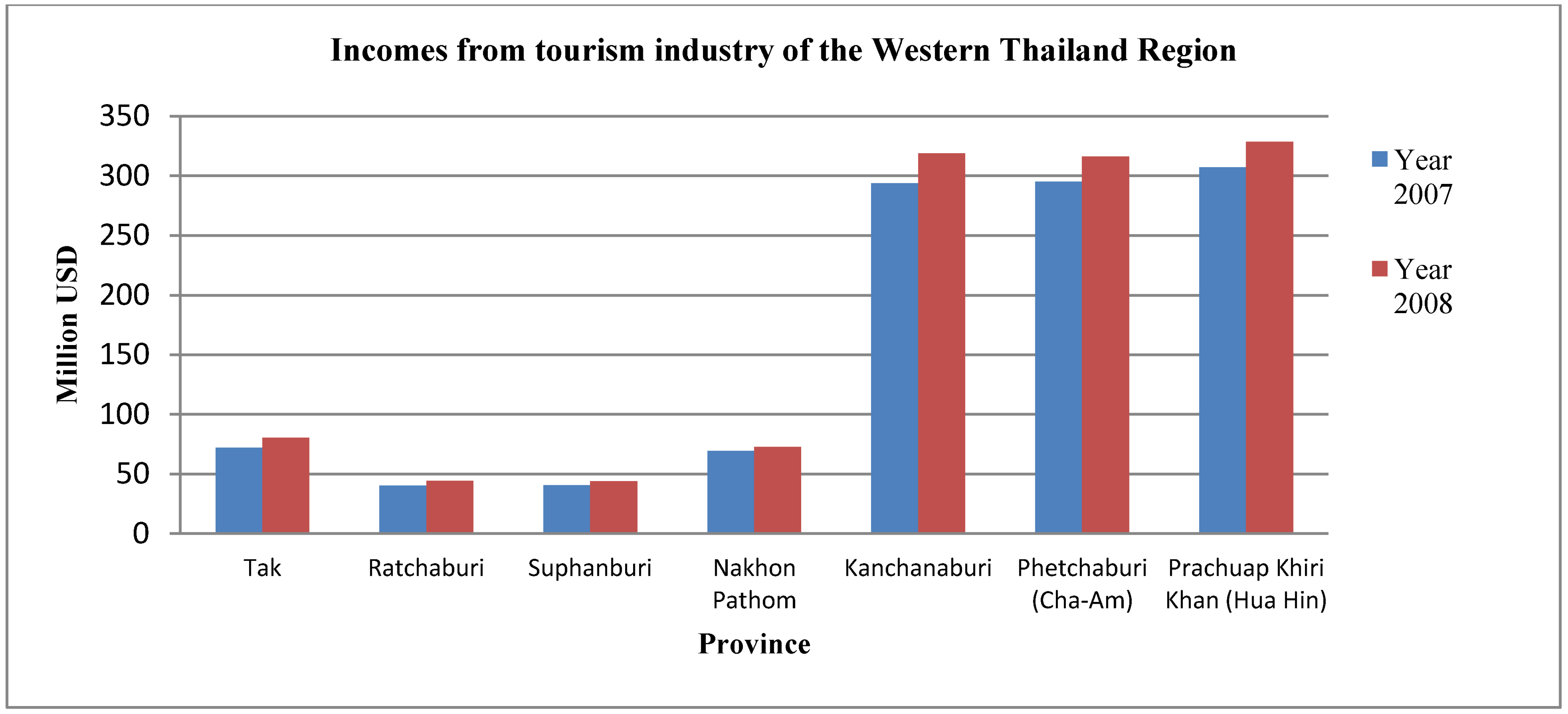
According to tourism statistics from the year 2008, Hua Hin had the highest number of tourist visits on the western side of the Gulf of Thailand. There is an income rate of around 329 US Dollar (
Figure 1). The internal tourism table has shown that the growth rate of the visitors increased by +73.94%. This statistic also indicates that the tourism industry in Hua Hin is booming and powerful enough to force the city’s growth, even though the local population of Hua Hin’s coastal urban region has not changed significantly. However, it also illustrates that the built-up area and many construction areas are expending because of the growth of the tourism industry. In total, 2,439,159 visitors came to Hua Hin in the year 2007, and the average length of stay was approximately 2.35 days per person. Thus, the rapid increase of the amount of accommodation and recreational sites in order to supply the tourists is one explanation for the city’s growth [
3].
Figure 1.
Income from tourism industry of Western Thailand.
Figure 1.
Income from tourism industry of Western Thailand.
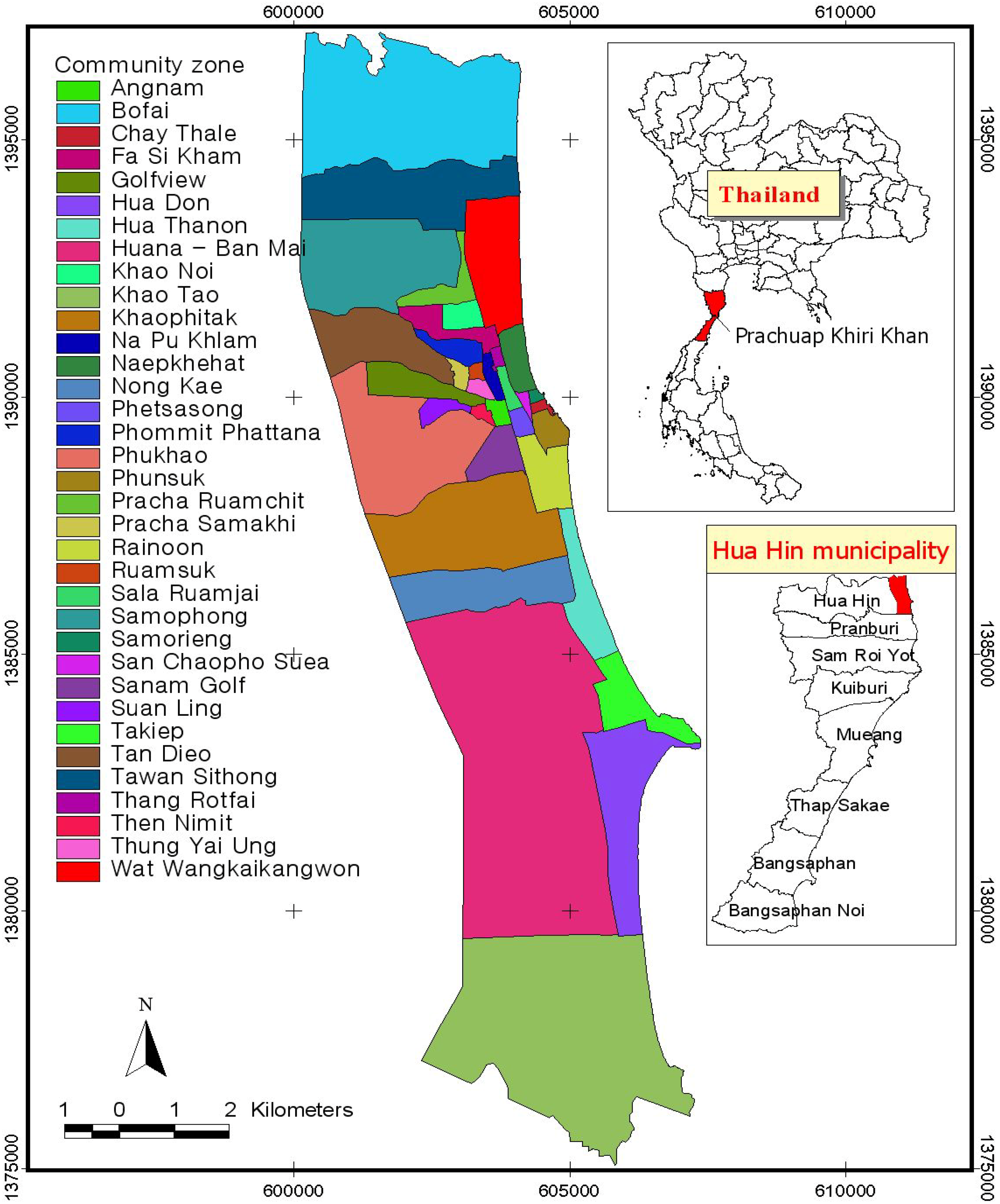
The study area is the seaside city of Hua Hin in the province of Prachuap Khiri Khan. It is located between latitudes 12°26' N and 12°38' N and longitudes 99°54' N and 100°00' N. It has a total area of 6,367.62 km
2 (636,762 hectares). Prachuap Khiri Khan province is famous in Thailand because it is the longest (distance 244 km) and narrowest coastal plain of Thailand and has several resources including the sea, beaches, waterfalls, and mountains. Hua Hin District is 838.96 km
2, while the Hua Hin municipality, where the core study area is, covers an area of 86.36 km
2. There are 35 communities within the Hua Hin municipality (see
Figure 2) [
3].
A report from the Hua Hin municipality office indicates that the increasing population has been caused mainly by immigration due to economic growth and the expansion of educational institutions. If we combine the population figures from the statistics from the Office of Tourism Development to recalculate the density of people per area, it is 46,972.13 people per square kilometers. This is an enormous increase in population for such a limited area and may affect the capacity of the city, such as the network transportation, public services and infrastructure, especially during the holiday season. In addition, Hua Hin has been a popular recreation place in Thailand for 100 years because the King and his family often visit Hua Hin, considering it the best recreational location in the country. Therefore, people visit Hua Hin because of its safety, calm sea, and beautiful beach. Hua Hin is also a pollution control area according to the National Environmental Board No. 13 (1996), and an area that is covered by environmental protection measures by the Ministry of Natural Resources and Environment Act 2000 [
3,
4].
Figure 2.
Study area: Hua Hin municipality and its communities.
Figure 2.
Study area: Hua Hin municipality and its communities.
Sustainable land use is of critical importance as we consider how to balance the needs of a growing population with the desire to protect our natural resources and environment [
5]. This paper presents an analysis of urban growth trends. Sustainable land use planners will be able to use the model to display the growth direction trend, as well as to discover how much the dynamic of land use change affects the place and its people. Land use planning is the systematic assessment of physical, social, and economic factors in such a way as to encourage and assist land users in selection options that increase their productivity, are sustainable, and meet the needs of society [
6].
The cellular automata model is a powerful tool to explain the direction of horizontal urban growth by using a lattice structure, state-space, neighborhoods, times and transition rules of pixels [
7]. This study tackles a challenging topic because it focuses on the direction of urban growth within a limited space; the area itself is a narrow coastal city. The northern side of the study area is the restricted area and includes the palace. The eastern side of the area is the sea, where the built-up area cannot be extended. The western part of the study area is a hill and the chief part of the southern area comprises a military zone.
2. Methods
2.1. Land Use and Land Cover Analysis
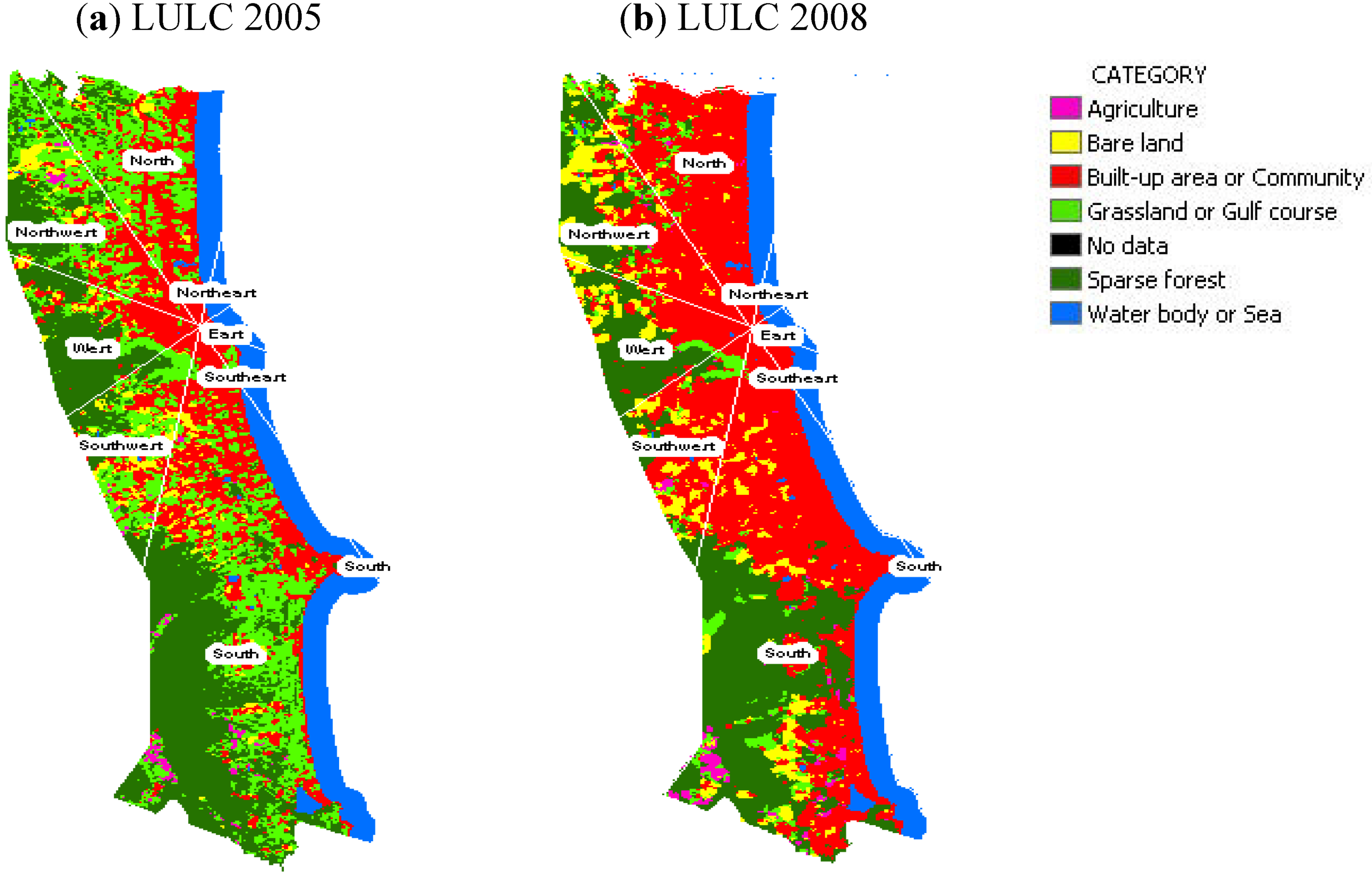
Land use and land cover patterns for 1999, 2002, 2005 and 2008 were mapped by the use of LANDSAT Thematic Mapper data (row/path: 51/139 for LANDSAT 4 MSS and row/path: 51/129 from LANDSAT 5 TM and LANDSAT 7 ETM+), which have a 30-m ground resolution (except for the thermal IR band (band 6), which has a 120-m resolution) and seven spectral bands. A modified version of the Anderson scheme of land use/cover classification was adopted the categories include: (1) water body or sea (2) urban or built-up area (3) agriculture (4) grassland or scrubland (5) bare land and (6) sparse forest.
The sensor is different from satellite data because it must process the geometric correction in order to correct the geometric distortions, both internal and external distortions. Internal distortions are caused by the sensor, such as lens distortion, disarrangement of detectors, variation of sampling rate, etc. External distortions are caused by external parameters other than the sensor, including variation of attitude and position of platform, earth curvature, topographic relief, etc. Geometric correction is undertaken to avoid geometric distortions from a distorted image, and is achieved by establishing the relationship between the image coordinate system and the geographic coordinate system using calibration data of the sensor, measured data of position and attitude, ground control points, atmospheric condition, etc. LANDSAT images were enhanced using linear contrast stretching and histogram equalization to improve the image to help identify ground control points in rectification. Images were rectified to a common UTM coordinate system based on 1:50,000 scale topographic maps. These data were resampled using the Nearest Neighbor algorithm, so that the original brightness values of pixels were kept unchanged.
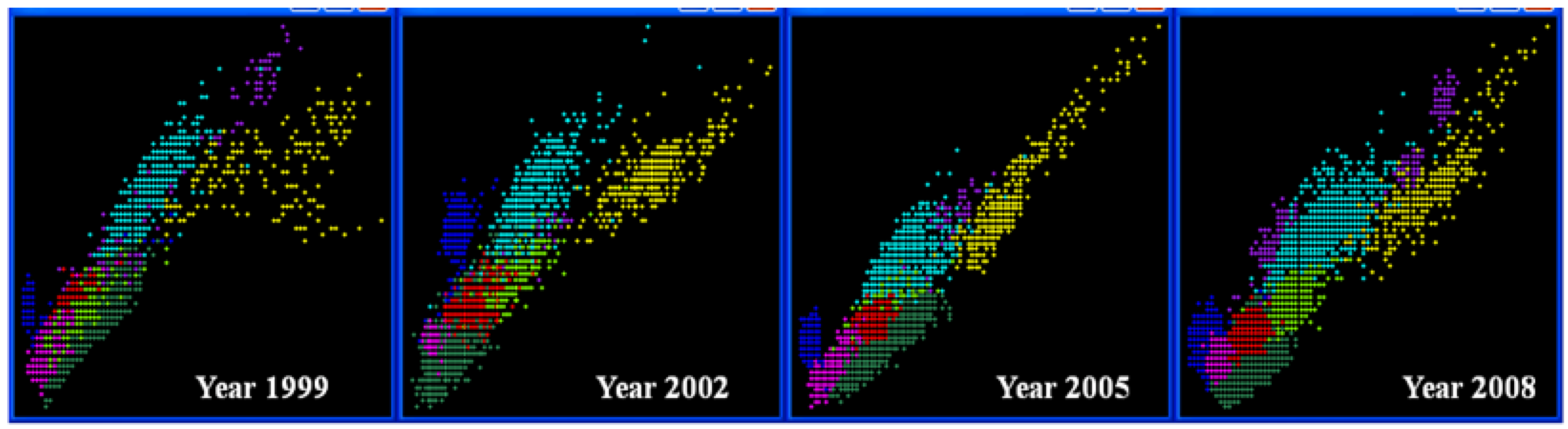
Supervised classification by the Maximum Likelihood technique was applied to classify the LANDSAT images. The 30 training areas were designed and drawn to scale at the same position in the raw image to reserve the pixel spectral of each land use class. In addition, the separability of each training area (
Figure 3) as a good representative of land use class was considered to calibrate the input data with the ground truth checks. The supervised classification image is well fitted with the representative pixel and can distinguish the land use class efficiently. The overall accuracy assessment from Maximum Likelihood technique (
Table 1) is 92.61 (year 1999), 91.93 (Year 2002), 95.88 (year 2005) and 98.59 (year 2008), respectively.
Figure 3.
The separability of the representative pixel of each training area (land use type).
Figure 3.
The separability of the representative pixel of each training area (land use type).
Table 1.
Accuracy assessment of Maximum Likelihood image classification.
Table 1.
Accuracy assessment of Maximum Likelihood image classification.
| Year | Overall Accuracy | Kappa Coefficient |
|---|
| 1999 | 92.61 | 0.9121 |
| 2002 | 92.93 | 0.9157 |
| 2005 | 95.88 | 0.9480 |
| 2008 | 98.59 | 0.9825 |
2.2. CA-Markov-Based Model
A raster data model is used in GIS to represent continuous data over space. The model divides the area into grid cells or pixels. Each grid cell is filled with the measured attribute values in a matrix and cell values are written in rows and columns. CA-Markov models represent an urban area with a lattice of cells, each of which exists in one of a finite set of states. The progression of time is modeled as a series of discrete steps with future patterns determined by transition rules which specify the behavior of cells over time [
7]. For example, a cell switches from undeveloped urban area (other land use type) to developed urban area, as a function of conditions at each cell and its neighboring cells at each time step. The pixel value of the raster data model in classified images and the simulated images from CA-Markov represents each land use type. The cell size determines the smallest unit or object that can be identified. The study assigned the cell size 25 sq.m. as the smallest unit of the built-up objects in the study area.
Using land use and cover change data derived from satellite images, this study also establishes the validity of the Markov process for describing and projecting land use and cover changes in the delta, by examining statistical independence, Markovian compatibility, and the states of the data. The Markov chain has
n states. The state vector is a column vector whose
ith component represents the probability that the system is in the
ith state at that time. Note that the sum of the entries of a state vector is 1. For example, vectors
X0 and
X1 in the above example are state vectors. If
pij is the probability of movement (transition) from one state j to state i, then the matrix
T = [pij] is called the transition matrix of the Markov chain [
7,
8,
9].
Theory gives the relation between two consecutive state vectors:
If Xn+1 and Xn are two consecutive state vectors of a Markov chain with transition matrix T, then Xn+1 = TXn.
If T is a regular transition matrix, then as n approaches infinity, Tn → S where S is a matrix of the form [v, v,…,v] with v being a constant vector.
If T is a regular transition matrix of a Markov chain process, and if X is any state vector, then as n approaches infinity, Tn X → p, where p is a fixed probability vector (the sum of its entries is 1), all of whose entries are positive.
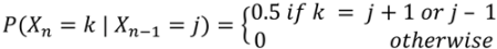
Consider a Markov chain with a regular transition matrix Markov process. An important class is Markov processes for which
For these processes, knowledge of the state of the system at time
tk provides all possible information about the state at any future time; information about the state at times before
tk is irrelevant. A deterministic analog is
- -
Future evolution of cell stateij = f(x) for x ≠ RN fully specified if full state x = x0 known at t = t0; state at earlier times is irrelevant.
- -
If only some subspace of x is known at t = t0, information about state at earlier times would be needed to specify trajectory.
Motion with position X
n on a lattice such that each time there is a 50% chance of moving one step either right or left.
where mean(x
n) = 0 (by symmetry), std(x
n) =
![Sustainability 05 01480 i005]()
variability of x
n grows without bound; size of fluctuations grows as square root of time.
The trend is a statistical approach to aid interpretation of data analysis. This study applies the trend value as a representative of the changing values from the probability of transition class and its transition area of each pair of the year’s output from the CA-Markov analysis. The trend values show that the probability of each land use type can possibly change to another land use type over the changing time period. The minus or plus values are the probability of the changing trend from each land use type to become another type during the time changes.
The IDRISI Sleva from Clark Lab (Clark University) is the software for simulating the land use change and the CA-Markov analysis. The CA-Markov analysis was run to test a pair of land cover images and outputs a transition probability matrix and a transition areas matrix. The transition probability matrix would explain the probability that each land cover category will change to every other category. The transition areas matrix is the number of pixels that are expected to change from each land cover type to every other land cover type over the specified number of time units.
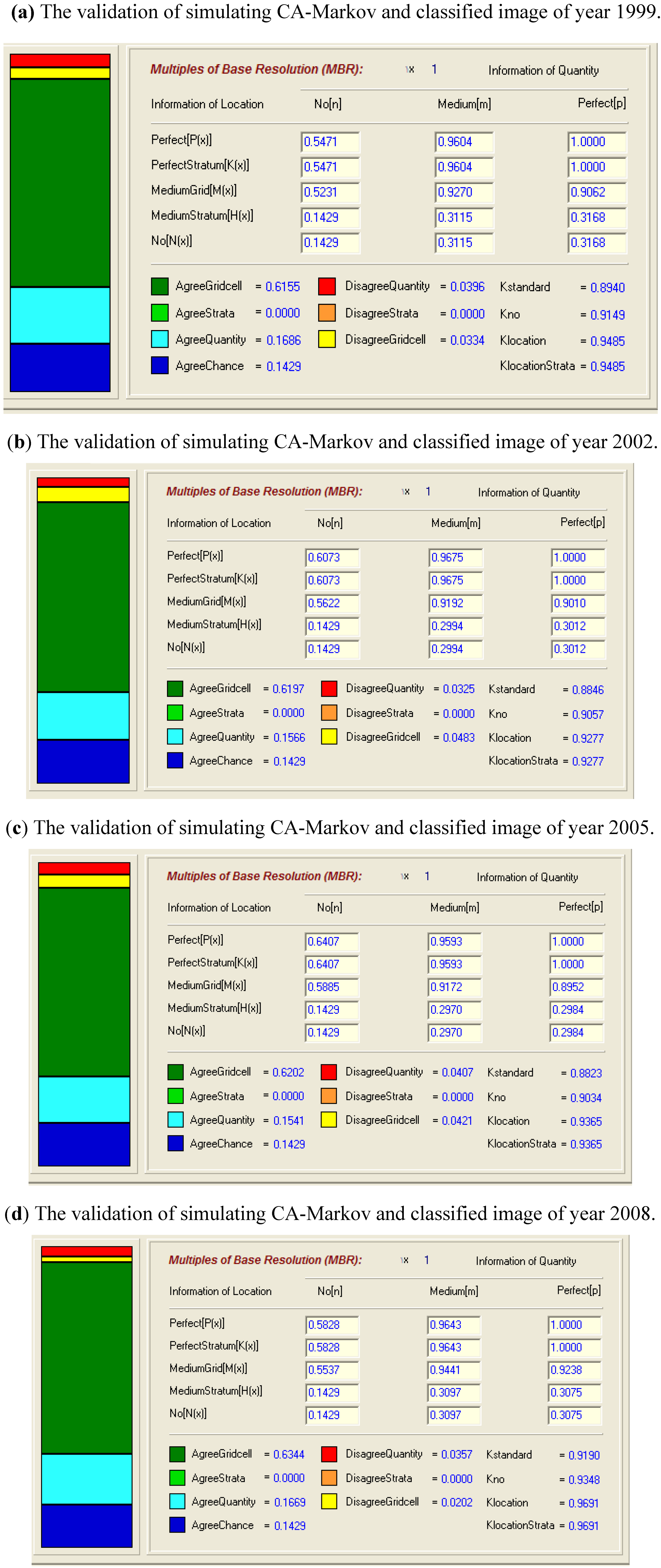
2.3. The Validation of Model Outputs
The purpose of validation of the output model is to monitor how well the actual data fit the model output. The validation offers one comprehensive statistical analysis that answers simultaneously two important questions: (1) How well do a pair of maps agree in terms of the quantity of cells in each category?; and (2) How well do a pair of map datasets agree in terms of the location of cells in each category? The model was validated using historical and reference land use datasets which were compiled [
10]. The validation procedure operates in two steps. Firstly, overall dynamics, system-wide features, and land use patterns are verified. Next, fine-tuning is carried out to get as many spatial details and pattern similarities as possible at the cellular level [
11].
The validation output (
Figure 4) is the components of agreement and disagreement based on the pair of images between the actual land use image from the classified image and the CA-Markov-simulated land use image.
Figure 4 displays the similarities and differences of each pair of images and indicates how they agree and disagree based on how they attribute each land use type in terms of both the quantity and location of the items. The accuracy of the model is the average value of the agreement and disagreement of the validated results based on both the percentage of correct results and the standard Kappa Index of Agreement mix disagreement of quantity with disagreement of location. The percent of accuracy from the simulated pixel and the actual pixel state (
Table 2) is 92.70 (year 1999), 91.92 (Year 2002), 91.72 (year 2005) and 94.41 (year 2008), respectively.
Table 2.
Percent of accuracy from simulated model.
Table 2.
Percent of accuracy from simulated model.
| Year | Percent of correct from CA-Markov | Kappa no. |
|---|
| 1999 | 92.70% | 0.9149 |
| 2002 | 91.92% | 0.9057 |
| 2005 | 91.72% | 0.9034 |
| 2008 | 94.41% | 0.9348 |
Figure 4.
Validation of model outputs.
Figure 4.
Validation of model outputs.
3. Results and Discussion
3.1. Urban Horizontal Expansion
This result describes the model testing for CA-Markov and data analysis for the creation of the model and its development. Spatially explicit models of land use change the focus to (Markov Chain Model) the rate of change between two or more classes, the location of change to one or more classes, and the rate and location of change between two or more classes. Models are usually calibrated using past time periods and/or hypotheses of the driving factors of change. The output may be the likelihood of each cell converting to a given class or predicted land use at one or more specified dates.
The pair of land use images has been selected to test into the Markov Chain Model (
Figure 6). In this case, land use of each year (1999 to 2002, 2002 to 2005 and 2005 to 2008) is selected to test the model. It is very simple, only needing land use at two time periods. However it does not consider drivers of change; it cannot be used over long time periods because of stationary transition values and it does not sufficiently differentiate between suitable locations. Thus, it is simply the primary testing of land use change between two time periods.
From the CA-Markov output (
Table 2,
Table 3,
Table 4,
Table 5,
Table 6) we have shown that the transition rule and probability of the land use class in an earlier year may change to another land use class in a later year. It shows urban horizontal expansion by using the probability of neighbor land use class which adjoins the existing urban or built-up area class and the dynamic direction of urban mobility by using the probability of neighboring land use type.
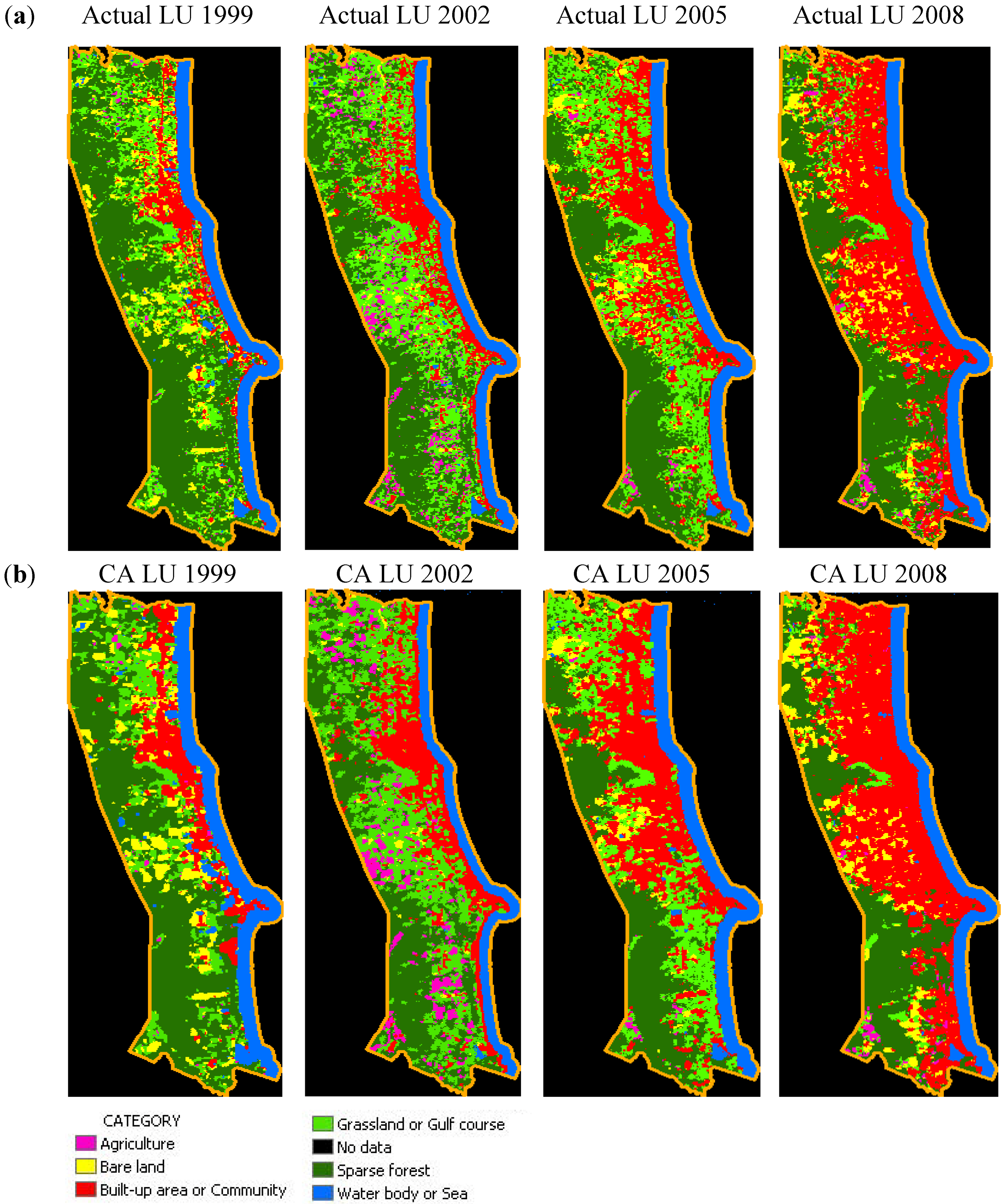
Figure 6.
Land use and land cover (LULC) change in different periods. (a) Actual LULC change from satellite image classification and field verification. (b) Simulated LULC change from CA-Markov modeling (CA LU).
Figure 6.
Land use and land cover (LULC) change in different periods. (a) Actual LULC change from satellite image classification and field verification. (b) Simulated LULC change from CA-Markov modeling (CA LU).
Comparing the simulated results from the CA-Markov analysis to the actual land use from image classification and field verification shows that they are rather similar. The validation result from the comparison between actual land use and the CA-Markov model outputs appear to show that it is acceptable and reliable. The validated outputs showed that the CA-Markov output and actual land use image match together in both the location of the cell state and its quantity.
Urban built-up areas show the extent of urban spaces. The built-up areas could characterize the spatial autocorrelation property, which may uncover the urban spatial pattern. Accordingly, spatial autocorrelation measures, including Moran I [
11], which indicates the probability of similar elements being located closely to each other, could be used to quantitatively measure urban sprawl patterns of urban cluster. The Moran’s Index was applied in order to test the propensity for data values to be similar to surrounding data values (cells).The measure used is Moran’s I, which ranges from −1 when adjacent cells are very dissimilar, to +1 when they are very much alike. The Moran I is positive when the observed value of locations within a certain distance or their contiguous locations tend to be similar, negative when they tend to be dissimilar, and approximately zero when the observed values are arranged randomly and independently over space.
The tested outputs indicate that the center cells state are similar to their adjacent cells. The spatial autocorrelation of the CA LU in each year is 0.9715 (year 1999), 0.9558 (year 2002), 0.9731 (year 2005), and 0.9665 (year 2008), respectively.
3.2. Directions and Trends of the City Growth Model
Direction relation is an important spatial relation. The descriptions and representations for direction relations have different levels of detail because of the varying dimensions of spatial objects [
12]. To identify the spatial direction of city growth from the CA model and the actual primary year of land use, the study area was divided into eight areas with the Central Business District (CBD) of Hua Hin downtown as the center point from which one can measure the direction of urban mobility.
Figure 6 (a) is the actual land use (LU) from the primary year while
Figure 6 (b) is the CA-Markov land use (CA LU) from simulation between actual land use of the primary year and the actual land use of the last year.
The matrix result shows how many possibilities there are by which class I (from column) in the previous land use image can change to be each class in the next period (time
t + n). The result shows that it is the possibility of a pixel in the year 1999 to be unchanged after a specific time period (three years). It shows how many pixels of land use in the year 1999 can change to be the state of another land use type in the year 2002, and so on. The percentage of escalating urban pixel of the CA LU in each year is 79.87% (years 1999 to 2002) (
Table 3), 75.73% (years 2002 to 2005) (
Table 5), and 86.48% (years 2005 to 2008) (
Table 7), respectively. This could be an accurate way of displaying the escalating image of urban growth of the Hua Hin municipality.
Table 3.
Probability of transition class of LULC 1999 to 2002.
Table 3.
Probability of transition class of LULC 1999 to 2002.
| 1999\2002 | Agriculture | Bare land | Built-up area | Grassland | Sparse forest | Water body | Percent |
|---|
| Agriculture | 23.02 | 0.71 | 6.03 | 43.81 | 25.95 | 0.48 | 100 |
| Bare land | 7.05 | 10.55 | 27.83 | 48.67 | 5.58 | 0.33 | 100 |
| Built-up area | 0.41 | 0.89 | 79.87 | 16.43 | 1.62 | 0.78 | 100 |
| Grassland | 13.17 | 1.77 | 10.21 | 48.13 | 26.61 | 0.12 | 100 |
| Sparse forest | 6 | 1.13 | 2.62 | 31.64 | 58.53 | 0.08 | 100 |
| Water body | 0.17 | 0.13 | 9.63 | 3.5 | 0.91 | 85.66 | 100 |
Table 4.
Transition area of each class of LULC 1999 to 2002.
Table 4.
Transition area of each class of LULC 1999 to 2002.
| 1999\2002 | Agriculture | Bare land | Built-up area | Grassland | Sparse forest | Water body | Total cell |
|---|
| Agriculture | 2018 | 63 | 529 | 3841 | 2275 | 42 | 8768 |
| Bare land | 187 | 279 | 737 | 1288 | 148 | 9 | 2648 |
| Built-up area | 81 | 179 | 15937 | 3278 | 324 | 155 | 19954 |
| Grassland | 5734 | 770 | 4445 | 20955 | 11587 | 51 | 43542 |
| Sparse forest | 2950 | 554 | 1289 | 15547 | 28763 | 38 | 49141 |
| Water body | 30 | 23 | 1697 | 617 | 160 | 15089 | 17616 |
| Total cell | 11000 | 1868 | 24634 | 45526 | 43257 | 15384 | 141669 |
| Changing Trend | 2232 | −780 | +4680 | +1984 | −5884 | −2232 | |
Table 5.
Probability of transition class of LULC 2002 to 2005.
Table 5.
Probability of transition class of LULC 2002 to 2005.
| 2002\2005 | Agriculture | Bare land | Built-up area | Grassland | Sparse forest | Water body | Percent |
|---|
| Agriculture | 5.87 | 6.91 | 15.38 | 49.55 | 22.11 | 0.18 | 100 |
| Bare land | 0.08 | 21.68 | 50.06 | 20.14 | 7.93 | 0.11 | 100 |
| Built-up area | 0.28 | 0.82 | 75.73 | 11.07 | 3.35 | 8.76 | 100 |
| Grassland | 0.79 | 8.55 | 27.47 | 40.8 | 22.02 | 0.37 | 100 |
| Sparse forest | 0.45 | 2.4 | 5.76 | 26.38 | 64.91 | 0.09 | 100 |
| Water body | 0 | 0.02 | 1.19 | 0.53 | 0.61 | 97.66 | 100 |
Table 6.
Transition area of each class of LULC 2002 to 2005.
Table 6.
Transition area of each class of LULC 2002 to 2005.
| 2002\2005 | Agriculture | Bare land | Built-up area | Grassland | Sparse forest | Water body | Total cell |
|---|
| Agriculture | 67 | 79 | 175 | 563 | 251 | 2 | 1137 |
| Bare land | 5 | 1356 | 3129 | 1259 | 496 | 7 | 6252 |
| Built-up area | 92 | 269 | 24829 | 3628 | 1098 | 2871 | 32787 |
| Grassland | 299 | 3241 | 10415 | 15465 | 8348 | 139 | 37907 |
| Sparse forest | 200 | 1067 | 2559 | 11718 | 28829 | 40 | 44413 |
| Water body | 0 | 3 | 227 | 101 | 118 | 18722 | 19171 |
| Total cell | 663 | 6015 | 41334 | 32734 | 39140 | 21781 | 141667 |
| Changing Trend | −474 | −273 | +8547 | −5173 | −5273 | +2610 | |
Table 7.
Probability of transition class of LULC 2005 to 2008.
Table 7.
Probability of transition class of LULC 2005 to 2008.
| 2005\2008 | Agriculture | Bare land | Built-up area | Grassland | Sparse forest | Water body | Percent |
|---|
| Agriculture | 29.82 | 17.85 | 15.66 | 23.39 | 13.28 | 0 | 100 |
| Bare land | 0.29 | 35.69 | 54.63 | 5.3 | 4.08 | 0.02 | 100 |
| Built-up area | 0.25 | 7.45 | 86.48 | 2.3 | 2.43 | 1.09 | 100 |
| Grassland | 3.31 | 8.52 | 45.67 | 16.29 | 26.14 | 0.07 | 100 |
| Sparse forest | 1.26 | 5.69 | 10.32 | 5.79 | 76.87 | 0.07 | 100 |
| Water body | 0.02 | 0.03 | 1.51 | 0.02 | 0.08 | 98.35 | 100 |
Table 8.
Transition area of each class of LULC 2005 to 2008.
Table 8.
Transition area of each class of LULC 2005 to 2008.
| 2005\2008 | Agriculture | Bare land | Built-up area | Grassland | Sparse forest | Water body | Total cell |
|---|
| Agriculture | 672 | 402 | 353 | 527 | 299 | 0 | 2253 |
| Bare land | 31 | 3797 | 5813 | 563 | 434 | 2 | 10640 |
| Built-up area | 135 | 4034 | 46812 | 1245 | 1318 | 589 | 54133 |
| Grassland | 334 | 861 | 4614 | 1646 | 2641 | 7 | 10103 |
| Sparse forest | 569 | 2577 | 4671 | 2621 | 34794 | 34 | 45266 |
| Water body | 3 | 5 | 292 | 4 | 15 | 18953 | 19272 |
| Total cell | 1744 | 11676 | 62555 | 6606 | 39501 | 19585 | 141667 |
| Changing Trend | −509 | +1036 | +8422 | −3497 | −5765 | +313 | |
However, the simulated model still has few errors because of the seasonal changes of the acquisition of the satellite imagery data. There are some differentiations of the land cover, such as changes in sea level or the water level in the reservoir, the abandonment of some community area, or a built-up area having some shrub cover. These factors affect the image classification to distinguish the land use types and the land use change through the time changes. When the actual land use types were compared to the simulated land use, they are deemed a disagreement of the cells’ state, in either quantity or location. This occurs, for example, when the water body changes to bare land as a result of sea level reduction over time, or when a built-up area or community abandons construction, and the area eventually turns to grassland and sparse forest. However, the output from the simulated land use model can strongly foresee the trend and a change in direction mobility so that the land use planning can still support the rapid growth of the tourism industry.
3.3. Direction from Trending of the Narrowest Coastal Urban Growth
A direction relation is an important spatial relation in GIS [
12] for land use planning. Since the analysis is based on the raster model in GIS, the direction of the cell space or the land use state must be defined clearly. The rectangle cell can be a partition. The extended lines of the boundary lines of the rectangle, which use X and Y axes as the width and height, respectively, are the axes of the partition. Therefore, the object or the cell center of each cell state (land use type) is divided into nine sub-regions to define inner, boundary, and ring direction relations. The direction of the study can be applied by placing the center at the original downtown area of Hua Hin, which is the center of the urban expansion.
From CA-Markov analysis, it can be seen that city growth has many growth directions. We found that the built-up area is growing and that its direction and the spatial direction are both positive compared to the actual land use in the year 1978.
At the beginning of actual land use analysis in the primary year, 1999, it seemed the growth direction would spread to the western side of the study area. However, the simulated model from CA shows that the land use of the years 2002 (
Figure 7), 2005 (
Figure 8), and 2008 (
Figure 9) spread to many of the western and southern areas.
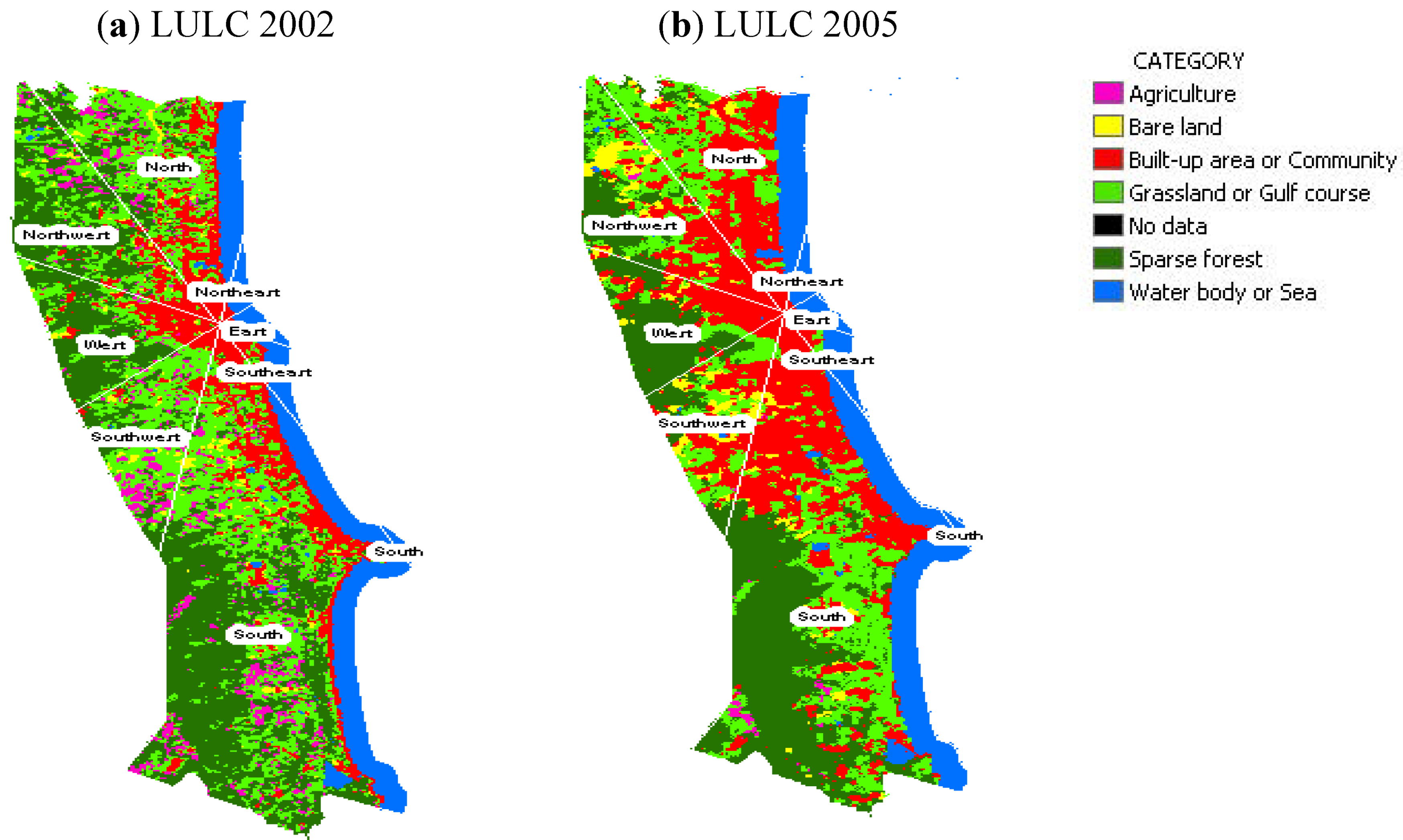
The political policy from Hua Hin municipality has encouraged changes in the direction of city growth. Comparing the actual land use from the primary years 2002, 2005 and 2008 with their CA-Markov models that were simulated from CA-Markov analysis, we found that the city growth direction spread less into the golf course in the western part of study area than the southern part, as it is a military area.
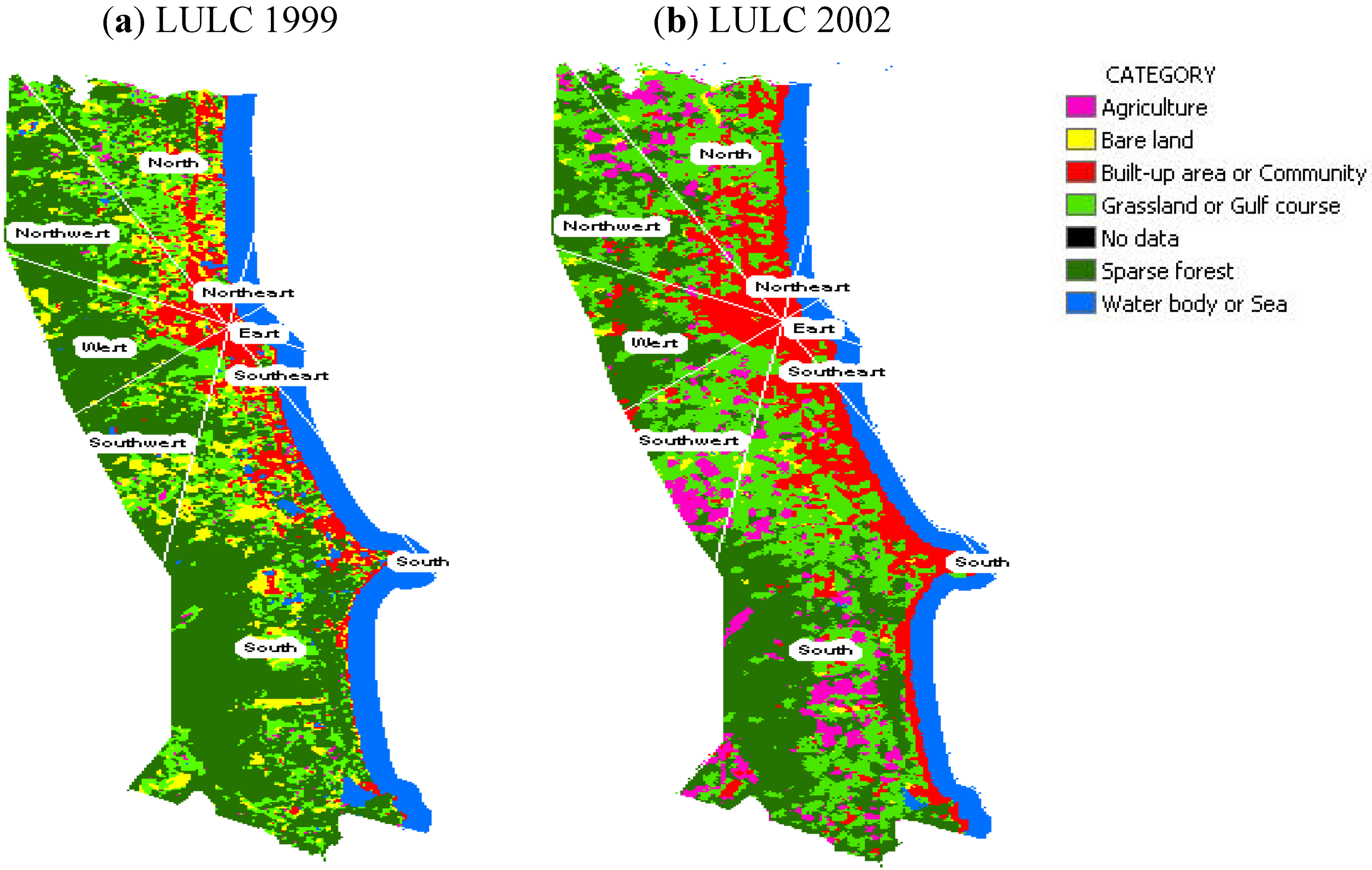
Figure 7.
Simulated land use and land cover change between the years 1999 to 2002.
Figure 7.
Simulated land use and land cover change between the years 1999 to 2002.
Figure 8.
Simulated land use and land cover change between the years 2002 to 2005.
Figure 8.
Simulated land use and land cover change between the years 2002 to 2005.
Figure 9.
Simulated land use and land cover change between the years 2005 to 2008.
Figure 9.
Simulated land use and land cover change between the years 2005 to 2008.
3.4. Spatial Decision Support from Mobility of Land Use Change and Its Trend for Sustainable Planning
From the CA-Markov analysis, the local planner can foresee the rapidity and the direction of urban expansion in order to plan for the capability resources to support people who live and visit this narrow seaside city. The tourism industry is particularly demanding, with huge usage being supported by limited resources.
It is accepted that computer modeling helps support the urban planner. Spatial decision support systems (SDSS) estimate the trend of urban growth, as well as the land use change around their local area, such as a municipality unit. GIS technology and its modeling statistics are especially useful in estimating the rate or ratio of changes [
13,
14,
15,
16,
17,
18,
19].
CA-Markov analysis output has shown that the transition rule and probability of the land use class in the earlier year may change to another land use class in a later year. It shows urban horizontal expansion by using the probability of neighbor land use class which adjoin the existing urban or built-up area class and the dynamic direction of urban mobility by using the probability of neighboring land use type.
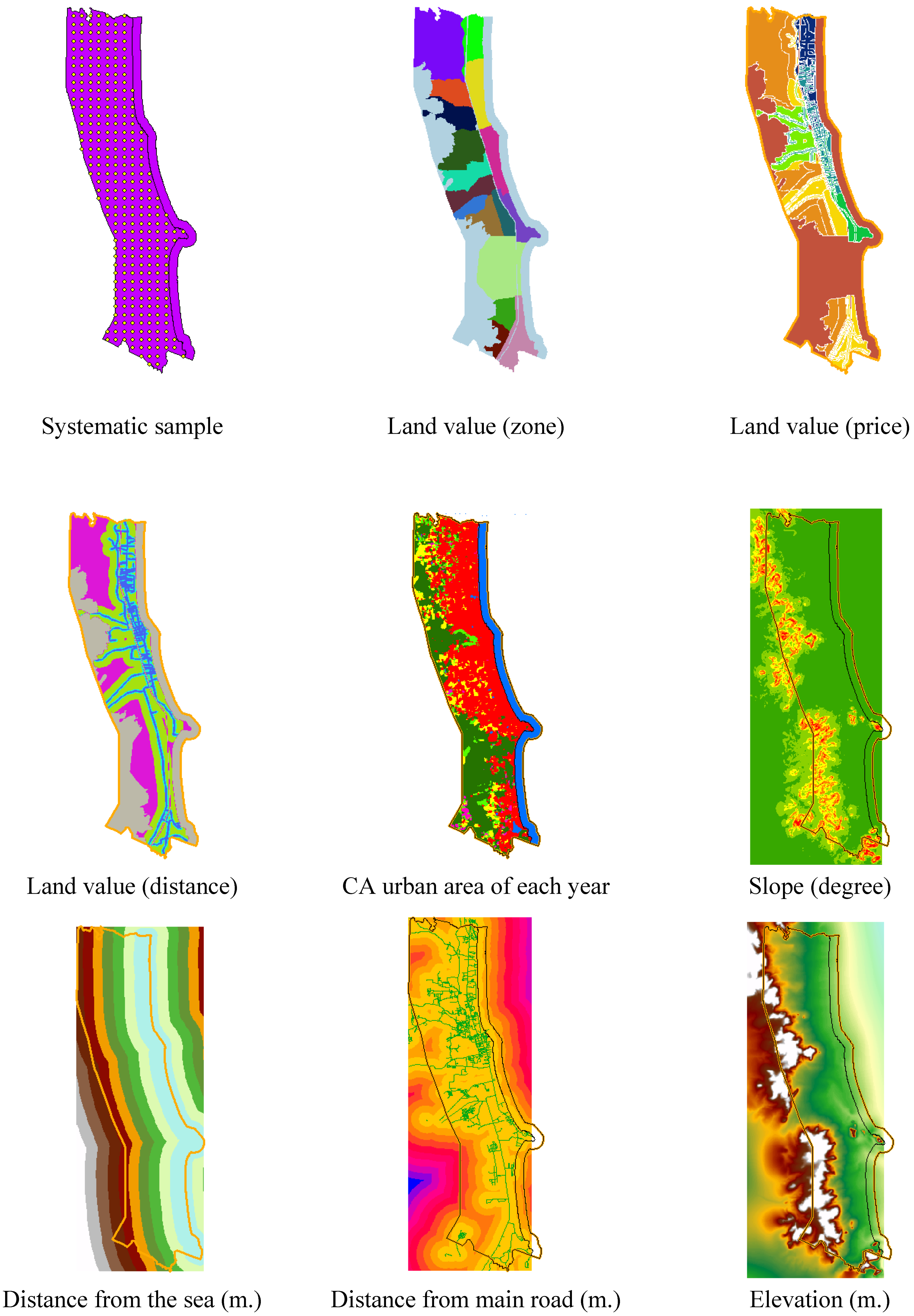
The variables (
Figure 5) that are used for the multiple regression analysis consist of the sample points of land value (zone), land value (price), land value (distance), CA-Markov urban area of each year, slope (degree), distance from the sea (m), distance from main road (m), and elevation (m). The backward elimination is applied for the selection of variables. The study found that six variables are not significant for urban horizontal expansion; namely, the land value by zone, land value by distance, distance from the sea, and the elevation of space.
In the meantime, there are only three variables, namely, the slope of the space, the land price, and the road distance, which are significant for the urban horizontal expansion of Hua Hin. The multiple regression analysis shows the regression model for horizontal expansion, as below (
Table 9).
Table 9.
Multiple regression analysis.
Table 9.
Multiple regression analysis.
| | Unstandardized Coefficients | | Standardized Coefficients | t | Sig. |
|---|
| Model | | B | Std. Error | Beta | | |
|---|
| 1 | (Constant) | 158.027 | 71.928 | | 2.197 | 0.011 |
| Slope | -115.44 | 21.438 | -0.179 | -5.385 | 0 |
| Land_Price | 4.527 | 0.084 | 0.216 | 6.311 | 0 |
| Road_Distance | 11.331 | 1.459 | 0.268 | 7.765 | 0 |
The equation can explain the local modeling of the urban growth expansion, especially the narrow coastal area along the sea, by using the model parameters for the physical factors to force expansion and settlement. More horizontal expansion will occur due to the low slope, higher land value, and farther road distance. The road distance is the most influential factor in forcing urban expansion and its growth because accessibility is very important for the long, narrow area. Meanwhile, the areas along the beach that are also connected to the main road are the expensive areas. However, the urban area still expands along either the main road or sub-main road. Because of its accessibility, the urban area is attractive for further business opportunity, and therefore the land use type will remain as an urban or built-up area, though the service function will be changed from a residential area to a commercial or business zone.
The price of the land is also an important factor in driving the direction of urban expansion, as well as influencing the rapidity of urban growth. The highest prices for land belong to the area along the beach. From the empirical study, the urban or the built-up area will be expanded to the cheaper land price and its function will be for residents. In contrast, the expensive price area near the beach will be changed from a residential area to a commercial, recreational or touristic area because of its accessibility. Many hotels, resorts, guesthouses and entertainment establishments are located in this area because tourists wish to relax near the beach with a nice atmosphere, where it is a calm and convenient to get to.
The low slope is another factor that affects the horizontal expansion, as the residential area could not be constructed on the steep slope and the legislation did not allow people to construct residences on the hill or mountain.
This study is only a part of the decision support system for modeling the land use situation. To plan local legislation, we need alternative modeling land use systems and an identification of problems or constraints, in order to determine the ranking of alternatives and make a final decision. In particular, we need to plan for the transportation network, energy and resource usage, pollution, and environmental concerns for the local inhabitants, as well as the rapid tourism development in the area of Hua Hin.
4. Conclusions
The CA-Markov model is used for studying urban growth in many contexts; one of the studies explores the narrowest coastal urban growth in Hua Hin city, Thailand. The results for the CA-Markov model output and the actual land use types are similar. The CA-Markov analysis shows a high interclass mobility, i.e., a high persistence of urban municipalities to stay in their own class from one decade to another. This means that CA-Markov can be applied to a study of many urban forms, even for constrained areas such as the narrow coastal area in the Hua Hin model.
This is, however, only a preliminary study of the urban expansion process of Hua Hin city; the city growth model is a complex phenomenon. Regardless, the study can provide a changing image of actual land use and simulated land use from CA-Markov that is useful for town planners and policy makers who can then decide on the direction of urban mobility, as well as the trend of urban growth.
Urban growth is a complex phenomenon and many factors influence it. Urban planning laws and regulations have influence on land development, especially in terms of urban expansion and protection of natural areas [
19]. The decision support system can be used for evaluating different planning options by using the performance indicators, which can be defined on the basis of the relevant planning agenda. CA-Markov and GIS technology are challenging tools to aid sustainable planning and development because they can illustrate the foreseeable phenomena [
19]. In addition, the study can predict the future growth of the narrow coastal areas in order to plan for the land use change under rapid tourism development. It is useful for planning the carrying capacity of the infrastructure service, waste management and transportation, as well as the construction of high buildings or tourist hotels in the future.


 variability of xn grows without bound; size of fluctuations grows as square root of time.