Measuring Carbon Emissions Performance in 123 Countries: Application of Minimum Distance to the Strong Efficiency Frontier Analysis

Abstract
:1. Introduction
2. Methodology
2.1. Strong Efficient Unit
2.2. Carbon Emissions Production Technology
 ,
,  ,
,  represent input, desirable output, and undesirable output variables, respectively. Assume
  as the unit under assessment and Fs(P) to be the strong efficient frontier of P. The minimum distance to the strong efficiency frontier problem may then be modeled as follows:

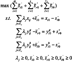
 represent the slack variables, M is a sufficiently large real number. The above problem is a linear bilevel programming problem (LBP), called (mSBM) to emphasize that it follows the idea of the SBM model [20], but minimizing instead of maximizing the L1-distance at the objective. Thus, it can offer the corresponding closest targets according to this distance. If the objective in the second program of Equation (2) is replaced as follows:
 ,
,  ,
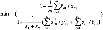
,  are, the better. Moreover, the denominators of these three values are constant. As long as the slack variables
  grow in size, the objective of Equation (3) will decrease. Therefore, the SBM represents the maximum distance to the strong efficiency frontier model.
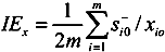
2.3. Carbon Emissions Performance Indexes
 are the inefficiency contribution ratios of the input, desirable output, and undesirable output respectively.
  ,
,  ,
,  are the percentages of improvement.

| DMU | x1 | x2 | x3 | y | b | θ | |
| 1 | original values | 28.1 | 4.6 | 31 | 12.6 | 6.3 | |
| SBM | 19.2 (32%) | 2.5 (46%) | 29.5 (5%) | 12.6 (0%) | 3.7 (40%) | 0.604 | |
| mSBM | 25.6 (9%) | 4.2 (10%) | 31 (0%) | 13.7 (9%) | 6.3 (0%) | 0.897 | |
| 4 | original values | 15 | 11.1 | 36.5 | 10.5 | 5.1 | |
| SBM | 15 (0%) | 3.9 (65%) | 26.8 (26%) | 10.5 (0%) | 2.7 (47%) | 0.564 | |
| mSBM | 15 (0%) | 8.8 (20%) | 36.5 (0%) | 12 (15%) | 2.2 (56%) | 0.687 | |
| 8 | original values | 19.8 | 4 | 23 | 9 | 5.1 | |
| SBM | 13.7 (31%) | 1.8 (55%) | 21 (8%) | 9 (0%) | 2.7 (47%) | 0.553 | |
| mSBM | 19.8 (0%) | 3.4 (16%) | 22.3 (3%) | 10 (12%) | 5.1 (0%) | 0.885 |
3. Empirical Analysis
3.1. Data and Its Descriptive Statistics Analysis
| Variable | Data compilation |
|---|---|
| Capital stock (K) | At current purchasing power parities (PPPs) (in millions at 2005 prices) |
| Labor force (L) | Number of persons engaged (in millions) |
| Energy consumption (E) | Refers to use of primary energy before transformation to other end-use fuels, which is equal to indigenous production plus imports and stock changes, minus exports and fuels supplied to ships and aircraft engaged in international transport. |
| Desirable output (Y) | Uses expenditure-side real GDP at chained PPPs (in millions at 2005 prices) |
| Undesirable output (b) | Uses Carbon dioxide emissions which are those stemming from the burning of fossil fuels and the manufacture of cement. They include carbon dioxide produced during consumption of solid, liquid, and gas fuels and gas flaring. |
| Variable | Unit | Mean | SD | Min | Max |
|---|---|---|---|---|---|
| K | $1 million | 1,851,566.30 | 5,381,598.77 | 9,693.44 | 41,251,352.00 |
| L | 106 workers | 23.06 | 83.02 | 0.17 | 777.38 |
| E | 103 tons | 92,995.80 | 293,928.85 | 799.60 | 2,257,100.88 |
| Y | $1 million | 524,979.04 | 1,535,226.62 | 5,136.00 | 12,839,243.00 |
| b | 103 tons | 239,703.89 | 866,647.14 | 1,485.14 | 7,687,113.77 |
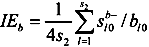
3.2. Carbon Emissions Comprehensive Performance
| No. | C.C. | θ | No. | C.C. | θ | No. | C.C. | θ |
|---|---|---|---|---|---|---|---|---|
| 1 | USA | 0.887 (26) | 42 | KAZ | 0.591 (114) | 83 | SVN | 0.837 (38) |
| 2 | CHN | 0.651 (102) | 43 | CHL | 0.859 (32) | 84 | CRI | 0.992 (3) |
| 3 | IND | 0.701 (83) | 44 | PER | 0.733 (74) | 85 | PAN | 0.96 (9) |
| 4 | JPN | 0.856 (34) | 45 | NOR | 0.905 (20) | 86 | URY | 0.898 (22) |
| 5 | DEU | 0.892 (25) | 46 | CZE | 0.757 (68) | 87 | BOL | 0.718 (76) |
| 6 | RUS | 0.62 (109) | 47 | PRT | 0.858 (33) | 88 | LUX | 0.979 (4) |
| 7 | FRA | 0.907 (18) | 48 | BGD | 0.761 (64) | 89 | CMR | 0.924 (11) |
| 8 | GBR | 0.96 (8) | 49 | QAT | 0.765 (62) | 90 | NPL | 0.871 (31) |
| 9 | BRA | 0.808 (47) | 50 | DNK | 0.894 (23) | 91 | LVA | 0.787 (53) |
| 10 | ITA | 0.907 (17) | 51 | ISR | 0.88 (28) | 92 | JOR | 0.606 (112) |
| 11 | MEX | 0.853 (35) | 52 | HUN | 0.826 (39) | 93 | PRY | 0.815 (43) |
| 12 | ESP | 0.893 (24) | 53 | FIN | 0.773 (57) | 94 | BIH | 0.682 (92) |
| 13 | KOR | 0.811 (45) | 54 | KWT | 0.756 (69) | 95 | ZMB | 0.67 (95) |
| 14 | CAN | 0.815 (44) | 55 | UZB | 0.622 (108) | 96 | CIV | 0.808 (48) |
| 15 | TUR | 0.924 (12) | 56 | IRL | 0.964 (7) | 97 | BRN | 0.915 (14) |
| 16 | IDN | 0.761 (65) | 57 | BLR | 0.667 (97) | 98 | BHR | 0.614 (110) |
| 17 | IRN | 0.686 (90) | 58 | IRQ | 0.638 (105) | 99 | TTO | 0.736 (73) |
| 18 | AUS | 0.811 (46) | 59 | NZL | 0.872 (30) | 100 | EST | 0.684 (91) |
| 19 | SAU | 0.682 (93) | 60 | MAR | 0.666 (98) | 101 | GEO | 0.695 (86) |
| 20 | POL | 0.743 (71) | 61 | SVK | 0.774 (56) | 102 | BWA | 0.845 (37) |
| 21 | NLD | 0.906 (19) | 62 | ECU | 0.703 (82) | 103 | ALB | 0.748 (70) |
| 22 | ARG | 0.759 (67) | 63 | LKA | 0.92 (13) | 104 | CYP | 0.801 (51) |
| 23 | THA | 0.673 (94) | 64 | BGR | 0.699 (84) | 105 | HND | 0.769 (59) |
| 24 | PAK | 0.761 (63) | 65 | OMN | 0.771 (58) | 106 | COD | 0.433 (123) |
| 25 | ZAF | 0.668 (96) | 66 | DOM | 0.796 (52) | 107 | MOZ | 0.512 (121) |
| 26 | EGY | 0.823 (41) | 67 | AZE | 0.602 (113) | 108 | GAB | 0.848 (36) |
| 27 | COL | 0.804 (50) | 68 | SDN | 0.975 (6) | 109 | SEN | 0.634 (106) |
| 28 | MYS | 0.71 (78) | 69 | AGO | 0.644 (103) | 110 | MKD | 0.651 (101) |
| 29 | BEL | 0.876 (29) | 70 | SYR | 0.565 (116) | 111 | TJK | 0.691 (87) |
| 30 | NGA | 0.467 (122) | 71 | HRV | 0.825 (40) | 112 | ARM | 0.713 (77) |
| 31 | UKR | 0.52 (120) | 72 | TUN | 0.766 (61) | 113 | MNG | 0.529 (119) |
| 32 | CHE | 0.977 (5) | 73 | ETH | 0.632 (107) | 114 | JAM | 0.706 (81) |
| 33 | SWE | 0.934 (10) | 74 | TKM | 0.573 (115) | 115 | MDA | 0.56 (117) |
| 34 | PHL | 0.767 (60) | 75 | GHA | 0.759 (66) | 116 | NAM | 0.805 (49) |
| 35 | AUT | 0.915 (15) | 76 | GTM | 0.91 (16) | 117 | KGZ | 0.698 (85) |
| 36 | VNM | 0.709 (79) | 77 | TZA | 0.688 (88) | 118 | BEN | 0.709 (80) |
| 37 | VEN | 0.652 (100) | 78 | LTU | 0.775 (55) | 119 | ISL | 0.737 (72) |
| 38 | ROU | 0.686 (89) | 79 | LBN | 0.64 (104) | 120 | COG | 0.719 (75) |
| 39 | HKG | 1 (1) | 80 | ZWE | 0.999 (2) | 121 | MLT | 0.881 (27) |
| 40 | GRC | 0.819 (42) | 81 | KEN | 0.785 (54) | 122 | SLV | 0.557 (118) |
| 41 | SGP | 0.898 (21) | 82 | YEM | 0.664 (99) | 123 | TGO | 0.609 (111) |

3.3. Carbon Emissions Inefficiency Analysis
| 1992 | 2009 | |||||||||
|---|---|---|---|---|---|---|---|---|---|---|
| E | L | K | Y | B | E | L | K | Y | b | |
| USA | 10.7% | 0% | 16.2% | 0% | 0% | 0.5% | 0% | 5.2% | 13.1% | 0% |
| (39.9%) | (0%) | (60.2%) | (0%) | (0%) | (2.5%) | (0%) | (27.8%) | (69.7%) | (0%) | |
| CHN | 0% | 89% | 0% | 0% | 0.5% | 27.4% | 0% | 0% | 8.9% | 87% |
| (0%) | (99.5%) | (0%) | (0%) | (0.52%) | (22.2%) | (0%) | (0%) | (7.2%) | (70.6%) | |
| IND | 0% | 2.8% | 0% | 0% | 90.4% | 0% | 81.8% | 0% | 0% | 9.9% |
| (0%) | (3%) | (0%) | (0%) | (97%) | (0%) | (89.2%) | (0%) | (0%) | (10.8%) | |
| JPN | 0% | 1.9% | 0% | 19.5% | 0% | 0% | 0% | 47.4% | 0% | 0% |
| (0%) | (8.8%) | (0%) | (91.2%) | (0%) | (0%) | (0%) | (100%) | (0%) | (0%) | |
| DEU | 0% | 0% | 31.8% | 0% | 0.4% | 0% | 0% | 30% | 0% | 0% |
| (0%) | (0%) | (98.7%) | (0%) | (1.3%) | (0%) | (0%) | (100%) | (0%) | (0%) | |
| RUS | 9.5% | 0% | 51.7% | 0% | 0% | 17.8% | 0% | 43.2% | 0% | 0% |
| (15.5%) | (0%) | (84.5%) | (0%) | (0%) | (29.1%) | (0%) | (70.9%) | (0%) | (0%) | |
| FRA | 20.2% | 10.8% | 0% | 0.2% | 0% | 0% | 0% | 24.7% | 3.75% | 0% |
| (64.8%) | (34.6%) | (0%) | (0.52%) | (0%) | (0%) | (0%) | (86.8%) | (13.2%) | (0%) | |
| GBR | 0% | 0% | 16.84% | 0% | 4.3% | 0% | 0% | 0% | 0% | 0% |
| (0%) | (0%) | (79.7%) | (0%) | (20.3%) | (0%) | (0%) | (0%) | (0%) | (0%) | |
| BRA | 0% | 0% | 60.1% | 0% | 0% | 0% | 0% | 0% | 37.4% | 12.7% |
| (0%) | (0%) | (100%) | (0%) | (0%) | (0%) | (0%) | (0%) | (74.6%) | (25.4%) | |
| ITA | 0.1% | 0% | 37% | 0% | 0% | 0% | 0% | 37.8% | 0% | 0% |
| (0.2%) | (0%) | (99.8%) | (0%) | (0%) | (0%) | (0%) | (100%) | (0%) | (0%) | |
| mean | 8.7% | 5.3% | 18.6% | 18% | 11.3% | 3.2% | 12.7% | 14.6% | 12.4% | 11.5% |
| (11.3%) | (7%) | (29.9%) | (30.2%) | (12.7%) | (4.3%) | (14.3%) | (27.7%) | (23.7%) | (16.2%) | |
3.4. Cluster Analysis
| Clustering by efficiency | Countries | Clustering by intensity | Countries |
|---|---|---|---|
| Carbon emissions high-efficiency zone | USA, JPN, DEU, FRA, GBR, ITA, MEX, ESP, TUR, NLD, EGY, BEL, CHE, SWE, AUT, HKG, SGP, CHL, NOR, PRT, DNK, ISR, HUN, IRL, NZL, LKA, SDN, HRV, GTM, ZWE, SVN, CRI, PAN, URY, LUX, CMR, NPL, BRN, BWA, GAB, MLT. | Carbon emissions low-intensity zone | USA, IND, JPN, DEU, FRA, GBR, BRA, ITA, MEX, ESP, KOR, CAN, TUR, IDN, AUS, NLD, ARG, THA, PAK, EGY, COL, MYS, BEL, CHE, SWE, PHL, AUT, VNM, HKG, GRC, SGP, CHL, PER, NOR, PRT, BGD, DNK, ISR, HUN, FIN, IRL, NZL, MAR, SVK, ECU, LKA, DOM, SDN, AGO, HRV, TUN, ETH, GHA, GTM, TZA, LTU, ZWE, KEN, SVN, CRI, PAN, URY, BOL, LUX, CMR, NPL, LVA, PRY, ZMB, CIV, BRN, GEO, BWA, ALB, CYP, HND, COD, MOZ, GAB, SEN, TJK, ARM, NAM, KGZ, BEN, ISL, COG, MLT, TGO. |
| Carbon emissions medium-efficiency zone | IND, BRA, KOR, CAN, IDN, IRN, AUS, SAU, POL, ARG, THA, PAK, ZAF, COL, MYS, PHL, VNM, ROU, GRC, PER, CZE, BGD, QAT, FIN, KWT, BLR, MAR, SVK, ECU, BGR, OMN, DOM, TUN, GHA, TZA, LTU, KEN, BOL, LVA, PRY, BIH, ZMB, CIV, TTO, EST, GEO, ALB, CYP, HND, TJK, ARM, JAM, NAM, KGZ, BEN, ISL, COG. | Carbon emissions medium-intensity zone | CHN, RUS, IRN, SAU, POL, NGA, VEN, ROU, CZE, KWT, BLR, BGR, OMN, LBN, YEM, JOR, BIH, EST, MKD, JAM, MDA, SLV. |
| Carbon emissions low-efficiency zone | CHN, RUS, NGA, UKR, VEN, KAZ, UZB, IRQ, AZE, AGO, SYR, ETH, TKM, LBN, YEM, JOR, BHR, COD, MOZ, SEN, MKD, MNG, MDA, SLV, TGO. | Carbon emissions high-intensity zone | ZAF, UKR, KAZ, QAT, UZB, IRQ, AZE, SYR, TKM, BHR, TTO, MNG. |
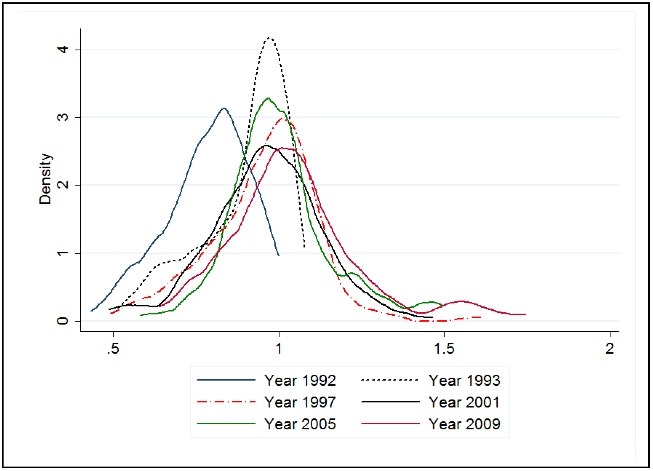
3.5. Convergence Analysis of ACECPI
4. Conclusions
Conflicts of Interest
References and Notes
- IPCC 2007. Available online: http://www.docin.com/p-731679800.html (accessed on 12 November 2013).
- Grossman, G.M.; Krueger, A.B. Economic growth and the environment. Q. J. Econ. 1995, 2, 353–377. [Google Scholar] [CrossRef]
- Tevie, J.; Grimsrud, K.M.; Berrens, R.P. Testing the Environmental Kuznets Curve Hypothesis for Biodiversity Risk in the US: A Spatial Econometric Approach. Sustainability 2011, 11, 2182–2199. [Google Scholar]
- Casler, S.D.; Rose, A. Carbon dioxide emissions in the US economy: a structural decomposition analysis. Environ. Resource. Econ. 1998, 11, 349–363. [Google Scholar] [CrossRef]
- Reinhard, S.; Lovell, C.A.K.; Thijssen, G.J. Environmental efficiency with multiple environmentally detrimental variables; estimated with SFA and DEA. Eur. J. Oper. Res. 2000, 2, 287–303. [Google Scholar] [CrossRef]
- Zhou, P.; Ang, B.W.; Poh, K.L. Slacks-based efficiency measures for modeling environmental performance. Ecol. Econ. 2006, 1, 111–118. [Google Scholar] [CrossRef]
- Guo, X.; Zhu, L.; Fan, Y.; Xie, B. Evaluation of potential reductions in carbon emissions in Chinese provinces based on environmental DEA. Energ. Pol. 2011, 5, 2352–2360. [Google Scholar]
- Zhang, Z.X. Macroeconomic effects of CO2 emission limits: A computable general equilibrium analysis for China. J. Pol. Model. 1998, 20, 213–250. [Google Scholar] [CrossRef]
- Kaya, Y.; Yokobori, K. Environment, Energy and Economy: Strategies for Sustainability; United Nations University Press: Tokyo, Japan, 1997. [Google Scholar]
- Mandal, S.K.; Madheswaran, S. Energy use efficiency of Indian cement companies: a data envelopment analysis. Energ. Effic. 2011, 1, 57–73. [Google Scholar] [CrossRef]
- Halog, A.; Manik, Y. Advancing Integrated Systems Modelling Framework for Life Cycle Sustainability Assessment. Sustainability 2011, 2, 469–499. [Google Scholar] [CrossRef]
- Jahanshahloo, G.R.; Vakili, J.; Zarepisheh, M. A linear bilevel programming problem for obtaining the closest targets and minimum distance of a unit from the strong efficient frontier. APJOR 2012, 2, 1–19. [Google Scholar]
- Zaim, O.; Taskin, F. Environmental efficiency in carbon dioxide emissions in the OECD: A non-parametric approach. J. Environ. Manag. 2000, 2, 95–107. [Google Scholar] [CrossRef]
- Ramanathan, R. A multi-factor efficiency perspective to the relationships among world GDP, energy consumption and carbon dioxide emissions. Technol. Forecast. Soc. Chang. 2006, 5, 483–494. [Google Scholar] [CrossRef]
- Zhou, P.; Ang, B.W.; Han, J.Y. Total factor carbon emission performance: A Malmquist index analysis. Energ. Econ. 2010, 1, 194–201. [Google Scholar] [CrossRef]
- Zhang, N.; Zhou, P.; Choi, Y. Energy Efficiency CO2 emission performance and technology gaps in fossil fuel electricity generation in Korea: A meta-frontier non-radial directional distance function analysis. Energ. Pol. 2013, 56, 653–662. [Google Scholar] [CrossRef]
- Lu, C.; Chiu, Y.; Shyu, M.; Lee, J. Measuring CO2 emission efficiency in OECD countries: Application of the Hybrid Efficiency model. Econ. Model. 2013, 32, 130–135. [Google Scholar] [CrossRef]
- Wang, K.; Yu, S.; Zhang, W. China’s regional energy and environmental efficiency: A DEA window analysis based dynamic evaluation. Math. Comput. Model. 2013, 58, 1117–1127. [Google Scholar] [CrossRef]
- Aparicio, J.; Ruiz, J.L.; Sirvent, I. Closest targets and minimum distance to the Pareto-efficient frontier in DEA. J. Prod. Anal. 2007, 3, 209–218. [Google Scholar] [CrossRef]
- Tone, K. A slacks-based measure of efficiency in data envelopment analysis. Eur. J. Oper. Res. 2001, 3, 498–509. [Google Scholar] [CrossRef]
- Cooper, W.W.; Ruiz, J.L.; Sirvent, I. Choosing weights from alternative optimal solutions of dual multiplier models in DEA. Eur. J. Oper. Res. 2007, 1, 443–458. [Google Scholar] [CrossRef]
- SPSS, version 17.0, SPSS Inc.: Chicago, IL, USA, 2009.
- Silverman, B.W. Density estimation for statistics and data analysis. CRC Press: Florida, FL, USA, 1986. [Google Scholar]
Appendix
© 2013 by the authors; licensee MDPI, Basel, Switzerland. This article is an open access article distributed under the terms and conditions of the Creative Commons Attribution license (http://creativecommons.org/licenses/by/3.0/).
Share and Cite
Wang, L.; Chen, Z.; Ma, D.; Zhao, P. Measuring Carbon Emissions Performance in 123 Countries: Application of Minimum Distance to the Strong Efficiency Frontier Analysis. Sustainability 2013, 5, 5319-5332. https://doi.org/10.3390/su5125319
Wang L, Chen Z, Ma D, Zhao P. Measuring Carbon Emissions Performance in 123 Countries: Application of Minimum Distance to the Strong Efficiency Frontier Analysis. Sustainability. 2013; 5(12):5319-5332. https://doi.org/10.3390/su5125319
Chicago/Turabian StyleWang, Ling, Zhongchang Chen, Dalai Ma, and Pei Zhao. 2013. "Measuring Carbon Emissions Performance in 123 Countries: Application of Minimum Distance to the Strong Efficiency Frontier Analysis" Sustainability 5, no. 12: 5319-5332. https://doi.org/10.3390/su5125319