Article

Land Change in the Mission-Aransas Coastal Region, Texas: Implications for Coastal Vulnerability and Protected Areas

Department of Geography, Texas A&M University, R 810 Eller O&M Building, College Station, TX 77843, USA
*
Author to whom correspondence should be addressed.
Sustainability 2013, 5(10), 4247-4267; https://doi.org/10.3390/su5104247
Submission received: 13 August 2013 / Revised: 17 September 2013 / Accepted: 18 September 2013 / Published: 26 September 2013

Abstract

:
The Mission-Aransas coastal region (MACR) in Texas is home to settlements vulnerable to coastal hazards. The region also contains significant biodiversity including several endangered species. The habitats in the bays and estuaries of MACR are especially sensitive to changes in land use/land cover (LULC) within the drainage basins upstream. We examine LULC change in the MACR from 1990 to 2010 and its implications for coastal vulnerability of the built environment and for the biodiversity in the region. Our findings show that, from 1990 to 2010, about a quarter of the MACR experienced LULC change. Developed land increased 71% (from 118 km2 in 1990 to 203 km2 in 2010), by far the greatest proportional change among all land cover classes. The rate of increase of developed land was slightly higher along the coast, 75% (from 65 km2 in 1990 to 114 km2 in 2010). Almost 90% of all developed land was within 50 km of the protected areas in both years. Overall, our findings point to increased exposure of the people and infrastructure to coastal hazards. Given the high social vulnerability in the study area, our study can inform formulation of sustainable management options that minimize both the coastal vulnerability of people and infrastructure and the pressure on the protected areas that are critical for conservation of biodiversity in the region.

1. Introduction

The change in land-use and land-cover (LULC), or more succinctly land change, is an integral component of global environmental change; hence, it is also a significant phenomenon to consider in moving towards global sustainability [1,2]. The transformation of land by human activities can disrupt biogeochemical cycles [3,4,5] and influence the vulnerability of people and infrastructure to various natural hazards [6,7,8]. LULC changes can alter the quantity and quality of freshwater resources [9,10,11], increase the potential for soil erosion [12,13], and lead to habitat loss and degradation [14,15].
In Texas, bays and estuaries are vital resources because these areas provide habitat for several fish and bird species of commercial and recreational value. A quarter of the state’s population resides in and a third of the state’s GDP comes from its estuary regions [16]. The state comes in fifth place in 24 coastal U.S. states in terms of participation rate in marine recreation [17]. However, the land changes in drainage basins upstream from these coastal areas can adversely affect these habitats due primarily to changes in water, sediment, and nutrient flows [18,19]. For example, the majority of nutrient loading to Texas estuaries arrive through freshwater inflows [20]. Moreover, as in other states along the Gulf of Mexico, Texas lost over half of its original wetland area by the 1980s (estimated to be 64,700 km2 circa 1780s) [21]. Increasing development, as well as tropical storms and changes in the geometry of coastlines due to sea-level rise and subsidence contribute to the loss and degradation of the state’s coastal wetlands [22,23]. In particular, urbanization along the coasts takes place mostly at the expense of agricultural lands and rangelands but it also puts under stress the already-diminished natural areas, some of which harbor remarkable biodiversity [24].
The combined impacts of sea-level rise, more-extreme precipitation, and tropical storm events due to anticipated climate change may lead to increased flooding along the Texas coastal region in the near future [25]. In addition, with the ongoing coastal development, the exposure and vulnerability of the people and infrastructure in the region to such hazards would increase. Exposure refers to the presence of people, infrastructure or other assets in an area where hazard events may occur [26]. Vulnerability is defined as the predisposition of people, infrastructure or other assets that are exposed to a certain hazard to be adversely affected by that hazard should it come to pass [26].
The Mission-Aransas coastal region (MACR) on the Coastal Bend of Texas is an area with a complex mix of different land uses including wetlands, woodlands, agricultural fields, and urban land [27]. The bays and estuaries in the Mission-Aransas region are especially sensitive to changes in land use/land cover (LULC) within the drainage basins upstream; these LULC changes can disrupt inputs of freshwater and material that are vital in maintaining salinity gradients, sedimentation rates, and nutrient cycles within the system [28]. These coastal areas are also sensitive to population increase, development, and change in agricultural activities within the watershed upstream. For these reasons, one of the National Estuarine Research Reserve (NERR) sites across the U.S., Mission-Aransas NERR, is established in this region [27,29]. The NERR System, supported through the National Oceanic and Atmospheric Administration (NOAA), is a network of 28 protected estuarine sites in the US and Puerto Rico [30]. One of the guiding principles of the NERR System is integrating “science, education and stewardship on relevant topics to maximize the benefits to coastal management” [31]. In addition, “understanding the long term effects of climate-change related processes on the estuary, including global warming, sea level rise, increased frequencies of tropical storms…” and “understanding the impact of future population increases and urbanization of the watershed and estuary” are two of the stated priority research issues within the Mission-Aransas NERR [29].
In this study, in line with the priorities of the Mission-Aransas NERR, we analyze the land changes in the MACR between 1990–2010 and the implications of these changes for the coastal vulnerability and the protected areas in the region. Specifically, we ask three questions:
(1).
What are the most prominent land changes that took place in the MACR?
(2).
How did the exposure of the built environment along the coast in the MACR to coastal hazards change?
(3).
Has there been an increase in the amount of urban land around the protected areas?

2. Study Area

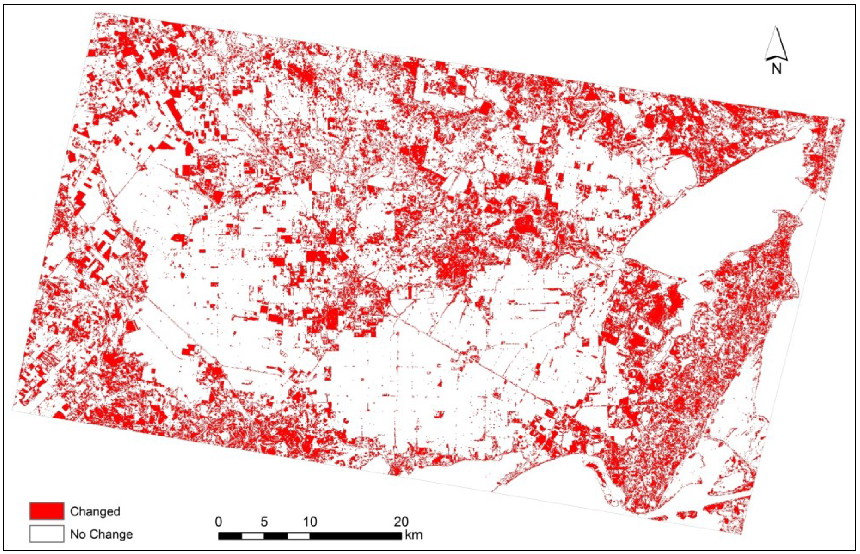
The Mission-Aransas coastal region (MACR) has an area of 3744 km2 (Figure 1). This area is approximately 30 miles north from the major urban center of Corpus Christi. Elevation in the region ranges from zero to 74 meters above sea level with most relief occurring in the northwestern portions. The MACR has a semi-arid climate with mean annual precipitation of 864 mm and a mean temperature of 21.8 °C. However, the distribution of annual precipitation is skewed by seasonal tropical storms that occasionally bring large amounts of rainfall [32]. Most of the MACR falls within the Aransas Watershed, but it also includes portions of the Mission and Nueces watersheds. The eastern portions of the MACR are characterized by coastal/near-shore environments that include all of Copano and Mission bays, as well as portions of Aransas, Nueces, Corpus Christi, and Red Fish bays (Figure 1). Central portions are mostly dominated by cultivated land with rangeland and woodland occupying much of the northern portions of the region [33].
Figure 1. Location map of the Mission-Aransas coastal region (MACR).
Sustainability 05 04247 g001
The MACR is predominantly rural with no large urban centers [33] (Table 1). Cities and towns are generally situated near the coast or streams; Portland, Ingleside, Rockport, and Aransas Pass are the largest urban areas (Table 1). The main industries consist of oil and gas activities, recreational and commercial fishing, ground and surface water withdrawal, tourism, and shipping [34]. The region is mostly at low elevation and its coastal areas face increasing risks from coastal hazards due to sea-level rise [35]. The mean sea level rise was recorded as 5.16 mm/yr from 1948 to 2006 at Rockport [36]. The current rate of sea level rise at Rockport is 5.50 mm/yr [37].
There are a number of protected areas in and around the study area. These areas are set aside for biodiversity conservation and they are especially concentrated near the coastline. The most important protected area in the region is the Mission-Aransas NERR, which is home to several endangered species including the iconic whooping crane (Grus americana) [38]. Since its establishment over four decades ago, the NERR System has collected a large amount of data on the socioeconomic and biophysical characteristics of their respective estuarine and coastal environments, valuable in addressing several resource-management issues [39]. Lately, the most significant issue facing NERR sites are impacts of land use and population growth [31]. Land change within NERR sites affect not only the hydrology but also the water quality within these sites [39].
Table 1. Settlements that fall within the Mission-Aransas Coastal Region (MACR) along with their population in 2010.
NameCountyDesignationPopulation in 2010
PortlandSan PatricioCity15,099
InglesideSan PatricioCity9387
RockportAransasCity8766
Aransas PassNueces/AransasCity8204
SintonSan PatricioCity5665
MathisSan PatricioCity4942
TaftSan PatricioCity3048
OdemSan PatricioCity2389
GregorySan PatricioCity1907
WoodsboroRefugioTown1512
FultonAransasTown1358
Ingleside on the BaySan PatricioCity615
San PatricioSan PatricioCity395
BaysideRefugioTown325
Total Urban Population63,612

3. Materials and Methodology

3.1. Data

We conduct image classification using Landsat Thematic Mapper (LTM) images for 1990 and 2010 as the primary input (Table 2). We use aerial photography for 1990, aerial photography/remote-sensor images from the early 1990s available through Google Earth™, National Land Cover Dataset (NLCD) maps for 1992, and Coastal Change Analysis Program (C-CAP) land-cover maps [40] for 1996 as reference data in the designation of training areas for the classification algorithm and independently in the accuracy assessment of the 1990 LULC image/map (Table 2). We spatially reference the aerial photos that we obtained from the United States Geological Survey (USGS) via Earth Explorer [41] by arranging each image such that the fiducial marks coincide with the coordinates specified in the respective metadata of each image. In addition, we use aerial photography for 2010 obtained from the Texas Natural Resources Information System (TNRIS) [42] and C-CAP LULC maps for 2006 as reference data in order to delineate training areas for the supervised classification algorithm, and in generating independent samples for the accuracy assessment of the 2010 LULC classified image. We also use a USGS National Elevation Dataset (NED) digital elevation model (DEM) of the study area at 10-m horizontal resolution to analyze the change in the amount of developed land that is exposed to coastal hazards. Finally, to quantify the change in developed land in the vicinity of the protected areas, we utilize the 2010 World Protected Area Database and include both the terrestrial and marine protected areas with International Union for Conservation of Nature (IUCN) status [43].

3.2. LULC Classification

The land-cover maps for the study site are available for years 1996 and 2006 from NOAA C-CAP [40]; however, since we aim to capture the land-change trends over a two-decade period, from 1990 to 2010, we carry out our own land-change analysis. We classify the northwestern portion of 1990 and 2010 LTM images independently using a modified Anderson Level I type of LULC scheme [44]. Specifically, we use seven LULC classes (Developed Land, Cultivated Land, Rangeland, Woodland, Open Water, Wetland, and Barren Land) in this analysis with slight differences in the naming scheme compared with Anderson Level I. The most apparent differences are in how the pasture and forest/woodland classes are treated. Anderson et al. (1976) [44] place pasture in the agriculture class, whereas we group pasture as part of the rangeland class. Hydrological properties of pasture are more similar to rangeland than cultivated crops in terms of the Soil Conservation Service runoff curve numbers (CNs) [45]. Thus, merging pasture class with rangeland class allows the LULC data generated in this analysis to be used as input data to a hydrological model [46]; In addition, the Anderson Level I scheme utilizes a forested land class, whereas in this analysis we utilize a woodland class instead because the MACR has a mix of trees and other woody vegetation. Due to the difficulty in separating large trees from other woody vegetation given the 30-m resolution of the LTM images, we aggregate these two classes into a single woodland class. We also use developed land label instead of urban or built-up land label of the Anderson system.
Image-preprocessing steps include co-registration, radiometric calibration, and atmospheric correction using the Fast Line-of-sight Atmospheric Analysis of Spectral Hypercubes (FLAASH) model in the Atmospheric Correction Module of ENVI [47]. FLAASH is a first-principles atmospheric correction tool that corrects wavelengths in the visible through shortwave infrared regions. By specifying the sensor type, FLAASH automatically incorporates some of the necessary parameters, but other parameters need to be specified that are dependent on the image and scene (Table 3). We utilize the U.S. Standard atmospheric and maritime aerosol models because the images were acquired in early spring (the other atmospheric models are specific to only the summer or winter) and because of the proximity of the MACR to the Gulf of Mexico.
Table 2. Data properties used in the image classification and accuracy assessment.
Name/ParameterDescriptionFormatSpatial ResolutionSource
LTM Image6 spectral bandsRaster30 mUSGS
for 17 March 1990
LTM Image6 spectral bandsRaster30 mUSGS
for 25 March 2010
Aerial PhotographyPanchromatic and color infraredRaster1 and 3 mUSGS
for 1989
Aerial PhotographyColor infraredRaster1 mTNRIS
for 2010
Google Earth ImageryPanchromatic and true colorRastervariousGoogle Earth
for 1990 and 1995
Land CoverAggregated to 7 classesRaster30 mNLCD
for 1992
Land CoverAggregated to 7 classesRaster30 mCCAP
for 1996
Land CoverAggregated to 7 classesRaster30 mCCAP
for 2006
National Elevation DatasetDigital Elevation Model (DEM)Raster10 mUSGS
LTM: Landsat Thematic Mapper scene (Row: 26, Path: 41); USGS Earth Explorer [41]; TNRIS: Texas Natural Resources Information System [42]; Google Earth; NLCD: National Land Cover Dataset; CCAP: Coastal Change Analysis Program.
After preproccessing, we classify the LTM images using the supervised Maximum Likelihood (ML) classifier [48]. The ML classification algorithm utilizes a probability-based decision rule; thus, for each pixel, the probability that that pixel belongs to each of a set of classes is determined and then the pixel is assigned to the class for which it has the highest probability of belonging. The ML procedure typically entails training areas for each class being specified within the respective image that is being classified (Table 4). The algorithm accrues probability information from remote-sensing training data via calculation of probability density functions [48]. To guide the selection of training areas, we use reference maps and images (Table 2), along with images of normalized difference vegetation index (NDVI) [49] and normalized difference water index (NDWI) [50]. In general, vegetation indices indicate green vegetation relative abundance; in particular, NDVI enhances features with higher reflectance in near-infrared (NIR) wavelength and lower reflectance in the red wavelength, such as terrestrial vegetation, whereas features with low red reflectance and very low NIR reflectance, such as water, are suppressed. In contrast, NDWI enhances water features while minimizing the effects of soil and terrestrial vegetation by exploiting reflected NIR radiation and visible green light [50]. Due to variations in wetland environments that cover a substantial amount of land within the MACR, NDVI and NDWI are integral in separating wetland vegetation from other forms of vegetation. We apply a 3-by-3 majority filter to the final output from the ML classification, where a pixel’s categorical (LULC) output value is defined by the category that appears most often amongst adjacent pixels (8 surrounding pixels), in order to minimize spuriously-classified pixels within the images. As a final step, we manually edit the pixels using the Spatial Pixel Editor in ENVI to change the classification of pixels that we know for certain are misclassified. The rationale for this classification post-processing is to generate maximally-accurate classification maps that can ultimately be used as input to hydrological models [46].
Table 3. Parameter specification for Fast Line-of-sight Atmospheric Analysis of Spectral Hypercubes (FLAASH) processing.
Parameter1990 Image2010 Image
Atmospheric ModelU.S. StandardU.S. Standard
Aerosol ModelMaritimeMaritime
Latitude for Scene Center27.434027.4340
Longitude for Scene Center−97.0670−97.0670
Average Ground Elevation for Scene (km)0.01700.0170
Initial Visibility (km)4040
Flight Date18 March 199025 Mar 2010
Flight Time in GMT16.300816.8089
Table 4. Count of pixels used as training areas for each land use/land cover (LULC) class for the image classification using the Maximum Likelihood classification procedure.
LULC ClassNumber of Training Pixels
1990 Image2010 Image
Developed Land44952099
Cultivated Land30,136115,240
Rangeland39083968
Woodland1491663
Open Water242,071149,832
Wetland43432477
Barren Land11712182

3.3. Accuracy Assessment and LULC Change

We assess the accuracy of the LULC images for 1990 and 2010 using reference images and maps obtained for the same year or from a year as close as possible to the year in which the assessed image was acquired (Table 2). Pre-processing is required for some of the reference images and maps before they can be used in the accuracy assessment: the aerial photography for 1989 has to be spatially referenced; 1992 NLCD maps and 1996 and 2006 C-CAP maps are aggregated to seven LULC classes similar to those used in this analysis (Table 5).
We utilize a stratified random sampling design with 50 samples per LULC class (total of 350 samples per image) in the accuracy assessment [51]. In order to quantitatively determine the accuracy of the 1990 and 2010 LULC maps, we compute error/confusion matrices. Using the error matrices, we compute three types of accuracy: producer’s, user’s, and overall accuracies, along with a standard Kappa index, commonly used in remote-sensing classification accuracy assessment [51]. However, Pontius and Millones (2011) have reported several issues regarding the use of Kappa indices, and they recommend using a method that quantifies both quantity disagreement and allocation disagreement [52]. Therefore, we also compute these two types of disagreement between reference data and classified images using the samples of pixels from the total number of pixels (population) to estimate the disagreement for the entire image. Inclusion of such measures in studies involving remote-sensing classification is important because more often than not the location of change is as important as the total amount of change across the land.
Table 5. Aggregated National Land Cover Data (NLCD) and Coastal Change Analysis Program (CCAP) land use/land cover (LULC) classes.
Aggregated LULC ClassOriginal NLCD LULC ClassOriginal CCAP LULC Class
1. Developed Land21. Low Intensity Residential2. Developed, High Intensity
22. High Intensity Residential3. Developed, Medium Intensity
23. Commercial/Industrial/Transportation4. Developed, Low Intensity
85. Urban/Recreational Grasses5. Developed, Open Space
2. Cultivated Land82. Row Crops6. Cultivated Crops
83. Small Grains
3. Rangeland51. Shrubland7. Pasture/Hay
71. Grassland/Herbaceous8. Grassland/Herbaceous
81. Pasture/Hay12. Scrub/Shrub
4. Forest Land/Woodland41. Deciduous Forest9. Deciduous Forest
42. Evergreen Forest10. Evergreen Forest
43. Mixed Forest11. Mixed Forest
5. Water11. Open Water21. Open Water
22. Palustrine Aquatic Bed
23. Estuarine Aquatic Bed
6. Wetland91. Woody Wetlands
92. Emergent Herbaceous Wetlands
13. Palustrine Forest Wetland
14. Palustrine Scrub/Shrub Wetland
15. Palustrine Emergent Wetland (Persistent)
16. Estuarine Forested Wetland
17. Estuarine Scrub/Shrub Wetland
18. Estuarine Emergent Wetland
7. Barren Land31. Bare Rock/Sand/Clay19. Unconsolidated Shore
32. Quarries/Strip Mines/Gravel Pits20. Barren Land
The LULC change from 1990 to 2010 is characterized for the MACR on a pixel-by-pixel basis. Using the change matrix, we compute the percent difference (PD) from 1990 to 2010 for each LULC class:
Sustainability 05 04247 i001
where A2010 is the areal coverage for a respective LULC class in 2010, and A1990 is the areal coverage for the same LULC class in 1990.

3.4. Low-Elevation Coastal Zone (LECZ) and Protected Area Analysis

In order to evaluate the expansion of the developed land along the coast during the study period, we create a low-elevation coastal zone (LECZ) map using a DEM of the study area at 10 m horizontal resolution. The low-elevation coastal zone (LECZ) is defined as “the contiguous area along the coast that is less than 10 m above sea level” [53]. The concentration of world population is the highest within the LECZ [54] and urban land expansion is occurring faster in this zone than in other areas around the world [6]. However, settlements in such lowlands are especially exposed, and the low-income groups in those settlements can be particularly vulnerable, to coastal hazards [53], the frequency and intensity of which may increase with climate change.
For the protected area (PA) analysis, we first identify the PAs with IUCN designation whose boundaries are within 50 km of the boundaries of the study area. Although these PAs have clearly defined boundaries and have formal management and protection measures in place [55], land changes including the expansion of developed land near PAs can significantly and negatively affect the ecosystem processes within them [56]. Therefore, we use 50 km as a first-order approximation for the width of the buffer zone within which land changes can have an influence on the ecological interactions within a PA and its surroundings [57]. Thus, we create buffer zones 50 km-wide around these protected areas. We then determine the developed land in the study area that falls within the buffer zones around the identified PAs.

4. Results

4.1. Accuracy Assessment of LULC

We use a sample of 50 reference sites per LULC class (350 total sites per image) to construct an error matrix for each LULC image generated in the classification procedure (Table 6). For 1990, the open water and cultivated land classes have the most agreement between the classified image and reference data. On the other hand, the woodland and wetland classes have the least amount of agreement between the classified image and reference data. This is mainly because the spatial resolution of LTM images makes it difficult to separate these classes from each other and other similar classes (e.g., woodland can be similar to rangeland, wetland can be similar to shallow water or vegetated areas with high soil moisture). For 2010, results are similar to 1990 with open water and cultivated land being the classes with the most agreement between the classified image and reference data. Also, woodland is the class with the least amount of agreement, as rangeland is commonly misclassified as woodland; this is not unexpected, as these two classes encompass some vegetation that can be relatively similar in terms of their spectra, and some areas are comprised of complex mosaics of the two classes. Furthermore, barren land has the second lowest amount of agreement because open water and wetlands are commonly misclassified as barren land. Barren land is commonly found at the interface of land and water (e.g., beaches and exposed soil near water bodies such as river banks). Thus, the disagreement could be influenced by variations in water elevations (e.g., tidal and river-flow fluctuations).
Table 6. Error matrix for (a) 1990 and (b) 2010 classified land use/land cover (LULC) image using 350 sample points.
(a)
(a)
Classified ImageryReference Imagery
DevelopedCultivatedRangelandWoodlandWaterWetlandBarrenRow Total
Developed4411001350
Cultivated0500000050
Rangeland2245100050
Woodland2143805050
Water0000500050
Wetland0206240050
Barren1130224150
Column Total49575345544844350
(b)
(b)
Classified ImageryReference Imagery
DevelopedCultivatedRangelandWoodlandWaterWetlandBarrenRow Total
Developed4314010150
Cultivated0491000050
Rangeland1443200050
Woodland00183205050
Water0000500050
Wetland1005341050
Barren3100453750
Column Total48556639584638350
We also use the error matrices to estimate the overall accuracy and parameters for the standard Kappa analysis. The 1990 image has an overall accuracy of 88.0%, whereas the 2010 image has an overall accuracy of 84.3% (Table 7a). The standard Kappa analysis involves computing an estimate of Kappa (KHAT), the variance of KHAT, and the standard normal Z-statistic for KHAT. A KHAT value greater than 0.80 is considered strong agreement between a classified image and reference data [51], and both the 1990 and 2010 LULC images have KHAT values greater than 0.80 (Table 7a). With the Z-statistic, it can be determined if the classified image is significantly better than one generated at random. The Z-statistics for the 1990 and 2010 image are 42.5 and 36.1 (Table 7a), respectively; hence, we conclude that the classified images are better than images generated at random even at a 99% confidence-level (Z-statistic = 2.58).
To further verify the accuracy of the 1990 and 2010 LULC images, we compute quantity and allocation disagreement using the 350 reference samples to estimate the overall agreement and quantity and allocation disagreement for the entire image (Table 7b). The disagreement between the classified image and reference data is again greater for the 2010 LULC image. The overall agreement for the 1990 and 2010 classifications is 93% and 89%, respectively (Table 7b). Furthermore, both types of disagreement are less than 10% for the 1990 and 2010 classified images.
Table 7. (a) Overall accuracy and estimates of Kappa parameters (variance and standard normal Z-statistic) for 1990 and 2010 land use/land cover (LULC) images. (b) Quantity and allocation disagreement statistics for 1990 and 2010 land use/land cover (LULC) images.
(a)
(a)
ImageOverall AccuracyKHATVar(KHAT)Z(KHAT)
1990 LULC88.0%0.860.0004142.5
2010 LULC84.3%0.820.0005136.1
(b)
(b)
ImageSamplePopulation
OverallQuantityAllocationOverallQuantityAllocation
AgreementDisagreementDisagreementAgreementDisagreementDisagreement
(%)(%)(%)(%)(%)(%)
1990 LULC88489334
2010 LULC84878947

4.2. LULC Change

Within the entire MACR, 25.5% of the total area experienced some form of LULC change. Areas that experienced change are spread throughout the MACR, but clusters of areas with the most change tend to be near water bodies (streams/rivers, estuaries, and bays) and urban centers. Among the land classes, rangeland is the class that experienced the greatest degree of LULC change, with much of the land being transformed to developed land. The most noticeable differences between the 1990 and 2010 LULC maps are significant expansions of woodland and developed land in the 2010 image (Figure 2). These have generally been at the expense of rangeland and cultivated land.
Developed land encompassed a relatively small proportion of the MACR area (3.2% and 5.4% for 1990 and 2010, respectively); it, nevertheless, increased 71%, the greatest proportional change among all classes (Table 8). Areas that changed to developed land are mostly found along the coast and outside urban areas such as Sinton and Portland. Clusters of areas that did not experience LULC change are those associated with large patches of cultivated land and water bodies (Figure 2 and Figure 3, Table 8).
Developed land increased by 84.3 km2 from 1990 to 2010, with most gains attributed to rangeland (54.7 km2) and woodland (41.8 km2), although it is surprising to note that a fair amount of developed land was lost to rangeland (21.9 km2) (Table 9). It is generally assumed that development does not transition back to vegetated land surface, but this disagreement could be due to abandonment and mapping/classification error. Cultivated land decreased by 101.0 km2, with most losses going to rangeland (123.2 km2), but it also gained some land from rangeland (41.8 km2) for a net loss of 81.4 km2 to rangeland. The large transitions between rangeland and woodland may be due to an overall greening of the MACR in the 2010 LTM image, relative to the 1990 LTM image and map error associated with the difficulty in separating these similar LULC classes using images at 30-m spatial resolution. Wetland increased by 30.7 km2, with most net gains coming from rangeland (22.3 km2) and woodland (16.3 km2), and a general net loss to other classes.
Figure 2. Map of land use/land cover (LULC) for Mission-Aransas coastal region (MACR) for (a) 1990, (b) 2010.
Sustainability 05 04247 g002
Table 8. Aerial coverage, percentage of total area that each land use/land cover (LULC) encompasses, and LULC change for the Mission-Aransas Coastal Region (MACR) in 1990 and 2010.
LULC Class19902010LULC Change
Area (km2)% of Total AreaArea (km2)% of Total AreaArea (km2)a% Changeb
Developed Land118.43.2%202.65.4%84.371.2%
Cultivated Land1375.636.7%1274.634.0%−101.0−7.3%
Rangeland1083.228.9%1029.027.5%−54.2−5.0%
Woodland370.99.9%396.010.6%25.16.8%
Open Water451.612.1%458.012.2%6.51.4%
Wetland287.37.7%318.08.5%30.710.7%
Barren Land57.51.5%66.11.8%8.715.1%
Total3744.4100.0%3744.4100.0%0.00.0%
a The net LULC change experienced by each class; b The percent change experienced by each LULC class.
Figure 3. Map of land use/land cover (LULC) change from 1990 to 2010 within the Mission-Aransas coastal region (MACR).
Sustainability 05 04247 g003
Table 9. Change matrix of land use/land cover (LULC) change from 1990 to 2010 for the Mission-Aransas Coastal Region (MACR).
2010 LULC (km2)
DevelopedCultivatedRangelandWoodlandWaterWetlandBarrenTotal
1990 LULC (km2)Developed67.56.921.99.10.78.14.2118.4
Cultivated20.71204.4123.26.20.513.86.71375.6
Rangeland54.741.8729.5195.30.956.84.31083.2
Woodland41.812.3111.3151.00.749.64.2370.9
Water0.40.00.00.0437.85.87.5451.6
Wetland7.85.234.533.312.3176.417.8287.3
Barren9.83.98.71.15.17.421.457.5
Total202.61274.61029.0396.0458.0318.066.13744.4

4.3. LECZ and PA Analyses

About 40% (or 1550 km2) of the total land area in the MACR lies within the LECZ. In 1990, about 65 km2 of developed land was within the LECZ, more than half of the total developed land in the MACR (Table 10). This proportion remained approximately the same by 2010, and the amount of developed land within LECZ increased to 114 km2, a 75% increase over the 20-year period. In contrast, the developed land outside the LECZ increased 67%. On the other hand, cultivated lands slightly decreased within the LECZ as in the rest of the study area (Table 10). Consequently, the percentage of cultivated lands that is in the LECZ remained virtually the same, at about 20%.
Due to the existence of, primarily, the Mission-Aransas NERR but also of other PAs, almost 90% of the MACR is within 50 km of the protected areas in the region. In MACR, developed land within 50 km of IUCN-designated PAs increased from 104 km2 in 1990 to 177 km2 in 2010. These findings do not change when we consider only those PAs with IUCN category I through IV, which are more critical for conservation of biodiversity [55]. As is the case for the whole study area, almost 90% of its developed land was within 50 km of the protected areas both in 1990 and 2010.
Table 10. Change in developed and cultivated land in the low-elevation coastal zone (LECZ) of MACR from 1990 to 2010.
Land use in MACRArea (km2) in …Change in area (%)
between 1990–2010
Percent in LECZ in …
1990201019902010
Developed53.288.767%55%56%
Developed in LECZ65.2113.975%
Cultivated1103.51011.2−8%20%21%
Cultivated in LECZ272.1263.2−3%

5. Discussion

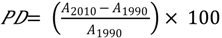
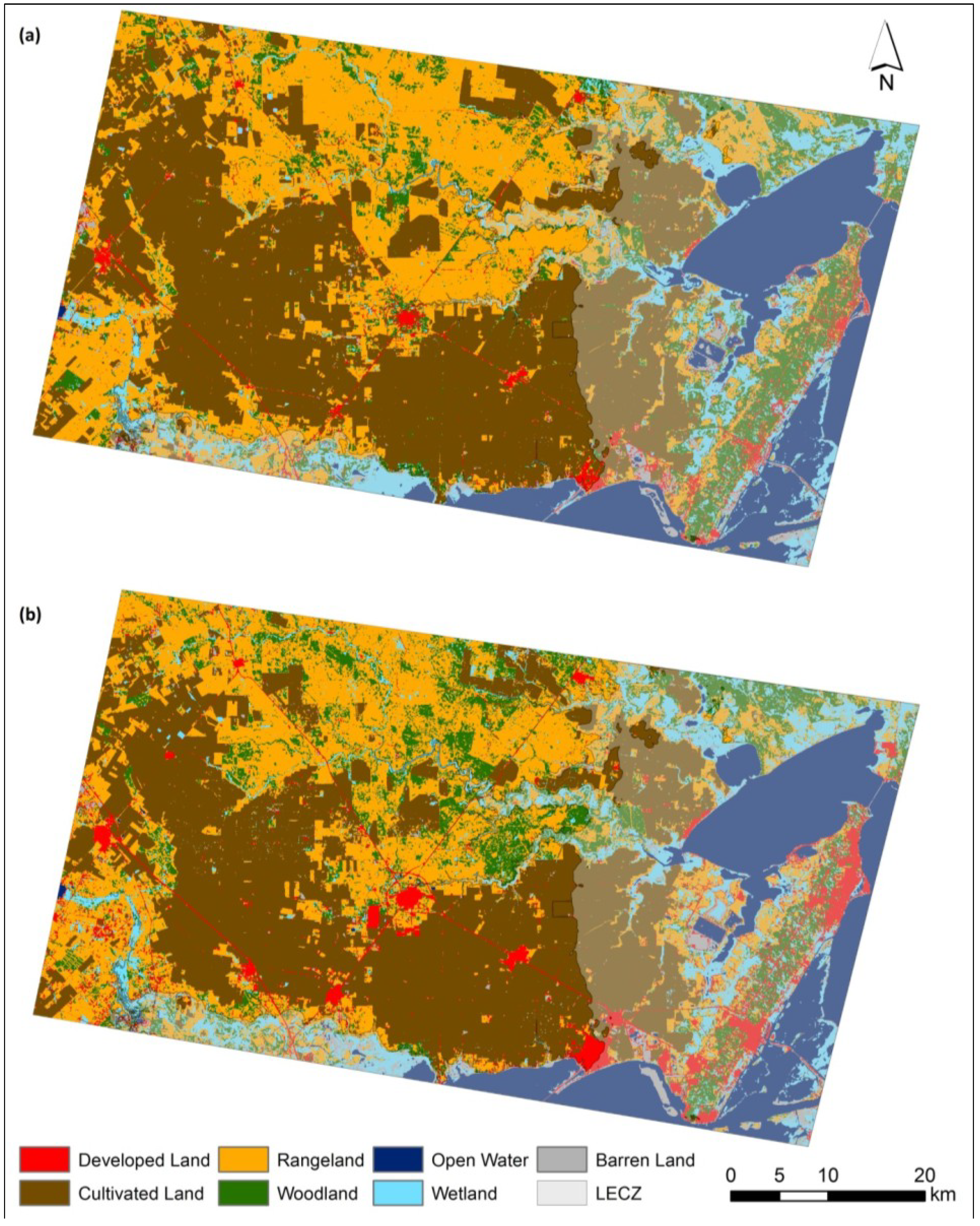
The MACR has no large urban centers, and it has a relatively sparse population. Nevertheless, anthropogenic activity has greatly influenced the biophysical characteristics of the landscape. A quarter of the study area underwent land change over the two-decade period. In particular, although it represents a modest proportion of the total area within MACR, the developed land nevertheless increased significantly. From 1990 to 2010, the developed land increased 71%, from 118 km2 to 203 km2 (Table 9). Over the same period, however, the population in the study area increased 14.5% [58].
The flat and low-lying Texas coastal plain has one of the highest rates of subsidence in the world [59] due to a combination of tectonics and anthropogenic activities [60]. Moreover, the potential increase in the frequency of storm surges elevates the risk of coastal flooding in the state [35] with detrimental effects on settlements, infrastructure, and habitats. While the frequency of tropical storms has remained fairly constant over time, their potential destructiveness has increased over the recent past and may continue to do so [61].
Our findings suggest a slightly higher rate of urban expansion in those lands that are deemed to be the most exposed to coastal hazards compared to more inland portions of the MACR. Much of this growth occurred in Rockport-Fulton and Aransas Pass on the Live Oak Peninsula (Figure 1 and Figure 2), which are already highly urbanized and have the highest population densities across the MACR. The low-elevation coastal zone (LECZ) defines, in approximate terms, the regions that are particularly exposed to the direct effects of sea level rise and storm surges as well as their potential indirect effects such as saline intrusion into groundwater aquifers [8,53]. The increasing concentration of infrastructure and people in these coastal areas oftentimes means potentially large losses of life as well as monetary losses in the case of a storm surge or coastal flooding. This is especially evident in mega-deltas of Asia such as the Mekong Delta [62] and Ganges-Brahmaputra [63]. Cultivated lands can also be adversely affected from storm surges and sea level rise both directly and indirectly through saline water intrusion [8,64]. We find that about one-fifth of all cultivated lands in the MACR remain within the LECZ and are hence exposed to coastal hazards.
Sediment flow, important in sustaining deltas and wetlands, has been altered by human activities across the world [65]. The decrease in its supply by rivers is also significantly impacting Texas coasts [66]. Indeed, in the MACR, this is one of the major factors that is thought to affect the habitat quality within the Mission-Aransas NERR protected area [28]. Continuing urbanization in the upper basins may initially lead to an increase in sediment supply but eventually lead to a sediment flow that is lower than that prior to urbanization [67]. Our findings reveal that the increase in the developed land in the upper basin has been marked and suggest that this trend may continue into the future with potentially adverse impacts on the biodiversity within the protected area. The decrease in sediment flow also increases the risk of coastal erosion, which can lead to the loss of the coastal and estuarine habitats as well as the increased exposure of the urban areas to coastal hazards.
A recent global study reported that the most urban land in the year 2000 near protected areas was in North America [68]. The MACR fits this pattern; almost all urban land in the region is within 50 km of the protected areas of the region, which were mostly established for conserving the regional biodiversity. The regulations that are in place minimize anthropogenic activities within the protected areas, such as the Aransas National Wildlife Refuge (ANWR), which is partly included within the Mission-Aransas NERR site. Nevertheless, those that occur near protected areas can still negatively impact these areas [56]. The ANWR is one of the areas in the region that harbor critical habitats of the endangered whooping cranes (Grus americana) [27].
In many parts of the world, socio-economic changes, in particular urbanization, appear to play a larger role in increasing exposure and vulnerability than anticipated increases in frequency and magnitude of extreme events due to climate change [69,70,71]. In Texas, the problems facing estuaries along the Gulf coast such as pollution and decrease in freshwater inflow due to population and development pressure extends back to at least the 1970s [72]. Likewise, the combined effects of socio-economic and biophysical changes increase the vulnerability of this region to coastal hazards in the MACR. A recent study identified populations in the MACR and its surrounding region as having high social vulnerability [73], which means these communities may bear disproportionate costs of adaptation to coastal hazards.
The increasing extent of impervious surfaces that typically characterize urban land may lower infiltration capacity of the land and thus decrease groundwater recharge. Therefore, the major concern with the development in the study area is its disruption of the hydrologic cycle via decreased infiltration and alteration of seasonal river flow patterns. In addition, urban and agricultural areas are often major sources of elevated nutrient levels in streams that reach coastal and estuarine habitats [74,75] with adverse effects on the biodiversity [75,76]. Elevated nutrient concentrations can have adverse effects on the biodiversity in these habitats. Moreover, the shoreline in the region is already experiencing shoreline retreat due mainly to insufficient supply of sediment to counter the erosion caused by storms, sea-level rise, and development [77]. Into the future, these issues are likely to be intensified as the effects of climate change become more apparent along the Texas coast in the form of sea-level rise [25]. However, the adaptation planning remains inadequate in the state where sea-level rise is rarely considered in decisions about coastal development [78]. One rare exception is the statewide Coastal Texas 2020 initiative, which aims to unite local, state, and federal efforts to promote the economic and environmental health of the Texas Coast [79]. Another is the research and community outreach efforts in and around the Mission-Aransas NERR site [29,80]. Nevertheless, the existing regulatory environment in the state risks large losses of life, property, and infrastructure in the face of anticipated increases in sea level [81].
A critical gap in our understanding is the interaction of land change with climate change and how this interaction impacts the sediment, nutrient, and freshwater flows in regions that are exposed to coastal hazards [64]. Closing this gap is important to ensure suitable habitat quality for the biodiversity in these regions, but is also important to improve the socio-economic conditions. Our findings provide important insights into the growing exposure and vulnerability of the urban areas in the MACR and of the Mission-Aransas NERR to coastal flooding due to land change and sea level rise. Quantifying and mapping LULC change in the region is the first step to accurately model the interaction of land cover and hydrological, sediment, and nutrient flows into the fragile ecosystems of the Mission-Aransas NERR site. Specifically, the LULC data outputs generated in this analysis can inform hydrological modeling of the MACR region to more accurately evaluate flooding risk as well as analyze changes in water quality due to the LULC change. Analyses of land changes such as this one can also inform land and other resource management decisions within the greater Mission-Aransas and Nueces region [82].

6. Conclusions

In this study, we examine the land-use/land-cover changes within the Mission-Aransas coastal region (MACR) on the Coastal Bend of Texas over the period of 1990–2010. Specifically, we determine the prominent land-change patterns and the implications of these patterns on the vulnerability of the urban residents and infrastructure to coastal hazards, and conservation of biodiversity in the MACR.
Our findings show that the MACR experienced a significant amount of LULC change over the last two decades. The MACR has been undergoing high rates of expansion of developed land. This growth may have increased the vulnerability of the urban residents and infrastructure to coastal hazards in the region. It has also meant more development in the vicinity of the protected areas such as the Aransas National Wildlife Refuge.
These trends are in line with global trends in urbanization, and each has significant implications for climate-change adaptation and biodiversity conservation in the region. The findings from this study also provide valuable input in determining the response of fluvial and coastal geomorphic systems to land change. Such analyses can help stakeholders develop more informed strategies for sustainable management of the Mission-Aransas NERR and its surroundings.

Conflicts of Interest

The authors declare no conflict of interest.

References and Notes

  1. Turner, B.L., II; Lambin, E.F.; Reenberg, A. Land change science special feature: The emergence of land change science for global environmental change and sustainability. Proc. Natl. Acad. Sci. USA 2007, 104, 20666–20671. [Google Scholar] [CrossRef]
  2. Foley, J.A.; DeFries, R.; Asner, G.P.; Barford, C.; Bonan, G.; Carpenter, S.R.; Chapin, F.S.; Coe, M.T.; Daily, G.C.; Gibbs, H.K.; et al. Global consequences of land use. Science 2005, 309, 570–574. [Google Scholar] [CrossRef]
  3. Webster, I.T.; Harris, G.P. Anthropogenic impacts on the ecosystems of coastal lagoons: Modelling fundamental biogeochemical processes and management implications. Mar. Freshwater Res. 2004, 55, 67–78. [Google Scholar] [CrossRef]
  4. Parfitt, R.L.; Scott, N.A.; Ross, D.J.; Salt, G.J.; Tate, K.R. Land-use change effects on soil C and N transformations in soils of high N status: Comparisons under indigenous forest, pasture and pine plantation. Biogeochemistry 2003, 66, 203–221. [Google Scholar] [CrossRef]
  5. Verchot, L.V.; Davidson, E.A.; Cattânio, J.H.; Ackerman, I.L.; Erickson, H.E.; Keller, M. Land use change and biogeochemical controls of nitrogen oxide emissions from soils in eastern Amazonia. Global Biogeochem. Cy. 1999, 13, 31–46. [Google Scholar] [CrossRef]
  6. Seto, K.C.; Fragkias, M.; Güneralp, B.; Reilly, M.K. A meta-analysis of global urban land expansion. PLoS ONE 2011, 6, e23777. [Google Scholar]
  7. Plate, E.J. Flood risk and flood management. J. Hydrol. 2002, 267, 2–11. [Google Scholar] [CrossRef]
  8. Qi, S.Z.; Qiu, Q.L. Environmental hazard from saltwater intrusion in the Laizhou Gulf, Shandong Province of China. Nat. Hazards 2011, 56, 563–566. [Google Scholar] [CrossRef]
  9. Kaushal, S.S.; Groffman, P.M.; Band, L.E.; Shields, C.A.; Morgan, R.P.; Palmer, M.A.; Belt, K.T.; Swan, C.M.; Findlay, S.E.G.; Fisher, G.T. Interaction between urbanization and climate variability amplifies watershed nitrate export in Maryland. Environ. Sci. Technol. 2008, 42, 5872–5878. [Google Scholar] [CrossRef]
  10. Wang, Z.; Zhang, B.; Zhang, S.; Li, X.; Liu, D.; Song, K.; Li, J.; Li, F.; Duan, H. Changes of land use and of ecosystem service values in Sanjiang Plain, Northeast China. Environ. Monit. Assess. 2006, 112, 69–91. [Google Scholar] [CrossRef]
  11. Zilberbrand, M.; Rosenthal, E.; Shachnai, E. Impact of urbanization on hydrochemical evolution of groundwater and on unsaturated-zone gas composition in the coastal city of Tel Aviv, Israel. J. Contam. Hydrol. 2001, 50, 175–208. [Google Scholar] [CrossRef]
  12. Yang, D.W.; Kanae, S.; Oki, T.; Koike, T.; Musiake, K. Global potential soil erosion with reference to land use and climate changes. Hydrol. Process. 2003, 17, 2913–2928. [Google Scholar] [CrossRef]
  13. Ward, P.J.; van Balen, R.T.; Verstraeten, G.; Renssen, H.; Vandenberghe, J. The impact of land use and climate change on late Holocene and future suspended sediment yield of the Meuse catchment. Geomorphology 2009, 103, 389–400. [Google Scholar] [CrossRef]
  14. Etter, A.; McAlpine, C.A.; Seabrook, L.; Wilson, K.A. Incorporating temporality and biophysical vulnerability to quantify the human spatial footprint on ecosystems. Biol. Conserv. 2011, 144, 1585–1594. [Google Scholar] [CrossRef]
  15. Harding, J.S.; Benfield, E.F.; Bolstad, P.V.; Helfman, G.S.; Jones Iii, E.B.D. Stream biodiversity: The ghost of land use past. Proc. Natl. Acad. Sci. USA 1998, 95, 14843–14847. [Google Scholar] [CrossRef]
  16. Colgan, C.S. The Value of Estuary Regions in the U.S. Economy. In The Economic and Market Value of Coasts and Estuaries: What’s At Stake? Pendleton, L.H., Ed.; Restore America’s Estuaries: Arlington, VA, USA, 2009; pp. 37–64. [Google Scholar]
  17. Leeworthy, V.R.; Wiley, P.C. Current Participation Patterns in Marine Recreation; US Department of Commerce, National Oceanic and Atmospheric Administration, National Ocean Service: Silver Spring, MD, USA, 2001; p. 47. [Google Scholar]
  18. Ji, J.H.; Chang, N.B. Risk assessment for optimal freshwater inflow in response to sustainability indicators in semi-arid coastal bay. Stoch. Env. Res. Risk A. 2005, 19, 111–124. [Google Scholar] [CrossRef]
  19. Merem, E.C.; Yerramilli, S.; Twumasi, Y.A.; Wesley, J.M.; Robinson, B.; Richardson, C. The applications of GIS in the analysis of the impacts of human activities on South Texas Watersheds. Int. J. Env. Res. Public Health 2011, 8, 2418–2446. [Google Scholar] [CrossRef]
  20. Yáñez-Arancibia, A.; Day, J.W. Environmental sub-regions in the Gulf of Mexico coastal zone: the ecosystem approach as an integrated management tool. Ocean Coast. Manage. 2004, 47, 727–757. [Google Scholar] [CrossRef]
  21. Dahl, T.E. Wetlands losses in the United States 1780’s to 1980’s; U.S. Department of the Interior, Fish and Wildlife Service: Washington, DC, USA, 1990; p. 13. [Google Scholar]
  22. Yáñez-Arancibia, A.; Day, J.W.; Reyes, E. Understanding the Coastal Ecosystem-Based Management Approach in the Gulf of Mexico. J. Coast. Res. 2013, Special Issue 63, 244–262. [Google Scholar] [CrossRef]
  23. Tietje, W.D.; Teer, J.G. Winter Feeding Ecology of Northern Shovelers on Freshwater and Saline Wetlands in South Texas. J. Wildl. Manage. 1996, 60, 843–855. [Google Scholar] [CrossRef]
  24. Buzan, D. Biodiversity in Texas’ Waters: Many Diverse Aquatic Ecosystems Support a Vibrant Fishery. Tex. Water Resour. 1997, 23, 1–12. [Google Scholar]
  25. Montagna, P.A.; Brenner, J.; Gibeaut, J.; Morehead, S. Coastal Impacts. In The Impact of Global Warming on Texas, 2nd ed.; Schmandt, J., North, G.R., Clarkson, J., Eds.; University of Texas Press: Austin, TX, USA, 2011; pp. 96–123. [Google Scholar]
  26. IPCC, Managing the Risks of Extreme Events and Disasters to Advance Climate Change Adaptation; A Special Report of Working Groups I and II of the Intergovernmental Panel on Climate Change; Cambridge University Press: Cambridge, UK; New York, NY, USA, 2012; p. 582.
  27. Evans, A.; Madden, K.; Palmer, S.M. The Ecology and Sociology of the Mission-Aransas Estuary: An Estuarine and Watershed Profile; University of Texas Marine Science Institute: Port Aransas, TX, USA, 2012; p. 183. [Google Scholar]
  28. Evans, A. Water Quality. In The Ecology and Sociology of the Mission-Aransas Estuary: An Estuarine and Watershed Profile; Evans, A., Madden, K., Palmer, S.M., Eds.; University of Texas Marine Science Institute: Port Aransas, TX, USA, 2012; pp. 33–45. [Google Scholar]
  29. NERRS. Mission-Aransas, TX. Available online: http://www.nerrs.noaa.gov/Reserve.aspx?ResID=MAR (accessed on 7 July 2013).
  30. NERRS. National Estuarine Research Reserve System: Overview. Available online: http://www.nerrs.noaa.gov/BGDefault.aspx?ID=61 (accessed on 14 July 2013).
  31. NERRS, National Estuarine Research Reserve System: Strategic Plan 2005–2010; NOAA, National Oceanographic and Atmospheric Administration: Silver Spring, MD, USA, 2006; p. 13.
  32. Schoenbaechler, C.; Guthrie, C.G. Coastal Hydrology for the Mission-Aransas Estuary. Available online: http://www.twdb.texas.gov/surfacewater/bays/major_estuaries/mission_aransas/doc/TWDB_Hydrology_MissionAransas_20110222.pdf (accessed on 16 July 2013).
  33. Morehead, S.; Beyer, T.G.; Dunton, K. Community Characterization of the Mission-Aransas National Estuarine Research Reserve and Surrounding Areas; University of Texas at Austin - Marine Science Institute: Port Aransas, TX, USA, 2007. [Google Scholar]
  34. Palmer, S.M.; Rose, C. Human Dimension. In The Ecology and Sociology of the Mission-Aransas Estuary: An Estuarine and Watershed Profile; Evans, A., Madden, K., Palmer, S.M., Eds.; University of Texas Marine Science Institute: Port Aransas, TX, USA, 2012; pp. 151–169. [Google Scholar]
  35. Atkinson, J.; McKee Smith, J.; Bender, C. Sea-Level Rise Effects on Storm Surge and Nearshore Waves on the Texas Coast: Influence of Landscape and Storm Characteristics. J. Waterway, Port, Costal, Ocean Eng. 2013, 139, 98–117. [Google Scholar] [CrossRef]
  36. Zervas, C. Sea Level Variations of the United States 1854–2006; NOAA, National Oceanographic and Atmospheric Administration: Silver Spring, MD, USA, 2009; p. 66. [Google Scholar]
  37. NOAA. Current Rates of Sea-Level Rise. Available online: http://tidesandcurrents.noaa.gov/sltrends/sltrends.shtml (accessed on 17 June 2013).
  38. Cook, C.; Palmer, S.M. Endangered Species. In The Ecology and Sociology of the Mission-Aransas Estuary: An Estuarine and Watershed Profile; Evans, A., Madden, K., Palmer, S.M., Eds.; University of Texas Marine Science Institute: Port Aransas, TX, USA, 2012; pp. 141–150. [Google Scholar]
  39. Mills, K.; Kennish, M.J.; Moore, K.A. Research and Monitoring Components of the National Estuarine Research Reserve System. J. Coast. Res. 2008, Special Issue 55, 1–8. [Google Scholar] [CrossRef]
  40. Digital Coast. Coastal Change Analysis Program Regional Land Cover. Available online: http://www.csc.noaa.gov/digitalcoast/data/ccapregional/ (accessed on 27 May 2013).
  41. USGS. Earth Explorer. Available online: http://earthexplorer.usgs.gov/ (accessed on 23 September 2012).
  42. TNRIS. Maps & Data. Available online: http://www.tnris.org/get-data (accessed on 1 October 2012).
  43. WDPA Annual Release. Available online: http://www.wdpa.org/ (accessed on 21 October 2012).
  44. Anderson, J.R.; Hardy, E.E.; Roach, J.T.; Witmer, R.E. A Land Use and Land Cover Classification System for Use with Remote Sensor Data; United States Government Printing Office: Washington, DC, USA, 1976; p. 41. [Google Scholar]
  45. Neitsch, S.L.; Arnold, J.G.; Kiniry, J.R.; Williams, J.R. Soil and Water Assessment Tool, Theoretical Documentation, Version 2009; Grassland, Soil and Water Research Laboratory - Agricultural Research Service, Blackland Research Center - Texas AgriLife Research: Temple, TX, USA, 2011; p. 618. [Google Scholar]
  46. Castillo, C.R. Modeling Impacts of Land-Use/Land-Cover Change and Variable Precipitation on Hydrology and Water Quality of a Coastal Watershed in Texas; Texas A&M University: College Station, TX, USA, 2013. [Google Scholar]
  47. ITT Visual Information Solutions. In Atmospheric Correction Module: QUAC and FLAASH User’s Guide; ITT: Boulder, CO, USA, 2009; p. 44.
  48. Jensen, J.R. Introductory Digital Image Processing: A Remote Sensing Perspective; Pearson Prentice Hall: Upper Saddle River, NJ, USA, 2005; p. 526. [Google Scholar]
  49. Rouse, J.W.; Haas, R.H.; Schell, J.A.; Deering, D.W. Monitoring Vegetation Systems in the Great Plains with ERTS. In Proceedings of the Third ERTS-1 Symposium NASA SP-351, Greenbelt, USA, 10–14 December 1973; Freden, S.C., Mercanti, E.P., Becker, M.A., Eds.; NASA: Greenbelt, MD, USA, 1974; pp. 309–317. [Google Scholar]
  50. McFeeters, S.K. The use of the Normalized Difference Water Index (NDWI) in the delineation of open water features. Int. J. Remote Sens. 1996, 17, 1425–1432. [Google Scholar] [CrossRef]
  51. Congalton, R.G.; Green, K. Assessing the Accuracy of Remotely Sensed Data: Principles and Practices; CRC Press: Boca Raton, FL, USA, 2009. [Google Scholar]
  52. Pontius, R.G., Jr.; Millones, M. Death to Kappa: Birth of quantity disagreement and allocation disagreement for accuracy assessment. Int. J. Remote Sens. 2011, 32, 4407–4429. [Google Scholar] [CrossRef]
  53. McGranahan, G.; Balk, D.; Anderson, B. The rising tide: assessing the risks of climate change and human settlements in low elevation coastal zones. Environ. Urban. 2007, 19, 17–37. [Google Scholar] [CrossRef]
  54. Small, C.; Nicholls, R. A global analysis of human settlement in coastal zones. J. Coast. Res. 2003, 19, 584–599. [Google Scholar]
  55. Dudley, N. Guidelines for Applying Protected Areas Management Categories; International Union for Conservation of Nature (IUCN): Gland, Switzerland, 2008; p. 86. [Google Scholar]
  56. Hansen, A.J.; DeFries, R. Ecological mechanisms linking protected areas to surrounding lands. Ecol. Appl. 2007, 17, 974–988. [Google Scholar] [CrossRef]
  57. DeFries, R.; Hansen, A.; Turner, B.L.; Reid, R.; Liu, J. Land use change around protected areas: Management to balance human needs and ecological function. Ecol. Appl. 2007, 17, 1031–1038. [Google Scholar] [CrossRef]
  58. USCB. American Fact Finder. Available online: http://factfinder2.census.gov/faces/nav/jsf/pages/index.xhtml (accessed on 7 April 2013).
  59. Anderson, J.B. Formation and Future of the Upper Texas Coast; Texas A&M Press: College Station, TX, USA, 2007; p. 163. [Google Scholar]
  60. Williams, S.J. Sea-Level Rise Implications for Coastal Regions. J. Coast. Res. 2013, 184–196. [Google Scholar] [CrossRef]
  61. Emanuel, K. Increasing destructiveness of tropical cyclones over the past 30 years. Nature 2005, 436, 686–688. [Google Scholar] [CrossRef]
  62. Smith, T.; Thomsen, D.; Gould, S.; Schmitt, K.; Schlegel, B. Cumulative Pressures on Sustainable Livelihoods: Coastal Adaptation in the Mekong Delta. Sustainability 2013, 5, 228–241. [Google Scholar] [CrossRef]
  63. Akanda, A.S.; Hossain, F. The climate-water-health nexus in emerging megacities. Eos Trans. AGU 2012, 93, 353–354. [Google Scholar] [CrossRef]
  64. Nicholls, R.J. Planning for the impacts of sea level rise. Oceanography 2011, 24, 144–157. [Google Scholar] [CrossRef]
  65. Syvitski, J.P.M.; Kettner, A.J.; Overeem, I.; Hutton, E.W.H.; Hannon, M.T.; Brakenridge, G.R.; Day, J.; Vorosmarty, C.; Saito, Y.; Giosan, L.; et al. Sinking deltas due to human activities. Nat. Geosci. 2009, 2, 681–686. [Google Scholar] [CrossRef]
  66. Ravens, T.M.; Thomas, R.C.; Roberts, K.A.; Santschi, P.H. Causes of salt marsh erosion in Galveston Bay, Texas. J. Coast. Res. 2009, 25, 265–272. [Google Scholar]
  67. Chin, A. Urban transformation of river landscapes in a global context. Geomorphology 2006, 79, 460–487. [Google Scholar] [CrossRef]
  68. Güneralp, B.; Seto, K.C. Futures of global urban expansion: uncertainties and implications for biodiversity conservation. Environ. Res. Lett. 2013, 8, 014025. [Google Scholar] [CrossRef]
  69. Dawson, R.J.; Ball, T.; Werritty, J.; Werritty, A.; Hall, J.W.; Roche, N. Assessing the effectiveness of non-structural flood management measures in the Thames Estuary under conditions of socio-economic and environmental change. Global Environ. Change 2011, 21, 628–646. [Google Scholar] [CrossRef]
  70. Storch, H.; Downes, N.K. A scenario-based approach to assess Ho Chi Minh City’s urban development strategies against the impact of climate change. Cities 2011, 28, 517–526. [Google Scholar] [CrossRef]
  71. De Moel, H.; Aerts, J.C.J.H.; Koomen, E. Development of flood exposure in the Netherlands during the 20th and 21st century. Global Environ. Change 2011, 21, 620–627. [Google Scholar] [CrossRef]
  72. Carter, L.J. Galveston Bay: test case of an estuary in crisis. Science 1970, 167, 1102–1108. [Google Scholar]
  73. Martinich, J.; Neumann, J.; Ludwig, L.; Jantarasami, L. Risks of sea level rise to disadvantaged communities in the United States. Mitig. Adapt. Strat. Gl. 2013, 18, 169–185. [Google Scholar] [CrossRef]
  74. Alexander, R.B.; Smith, R.A.; Schwarz, G.E.; Boyer, E.W.; Nolan, J.V.; Brakebill, J.W. Differences in phosphorus and nitrogen delivery to the Gulf of Mexico from the Mississippi River Basin. Environ. Sci. Technol. 2008, 42, 822–830. [Google Scholar]
  75. Carpenter, S.R.; Caraco, N.F.; Correll, D.L.; Howarth, R.W.; Sharpley, A.N.; Smith, V.H. Nonpoint pollution of surface waters with phosphorus and nitrogen. Ecol. Appl. 1998, 8, 559–568. [Google Scholar] [CrossRef]
  76. Meyer, J.L.; Paul, M.J.; Taulbee, W.K. Stream ecosystem function in urbanizing landscapes. J. N. Am. Benthol. Soc. 2005, 24, 602–612. [Google Scholar]
  77. McKenna, K.K. Texas Coastwide Erosion Response Plan: 2009 Update; Texas General Land Office: Austin, TX, USA, 2009; p. 86. [Google Scholar]
  78. Dolan, G.; Wallace, D.J. Policy and management hazards along the Upper Texas coast. Ocean Coast. Manage. 2012, 59, 77–82. [Google Scholar] [CrossRef]
  79. TGLO, Coastal Texas 2020: Executive Summary; Texas General Land Office: Austin, TX, USA, 2005; p. 17.
  80. Madden, K.; Morehead, S. Mission-Aransas NERR Ecosystem Based Management Tool Demonstration Project: An Integrated Approach to Land Use Planning in Aransas County; University of Texas Marine Science Institute: Port Aransas, TX, USA, 2011; p. 37. [Google Scholar]
  81. McLaughlin, R.J. Rolling easements as a response to sea level rise in coastal Texas: Current status of the law after Severance v. Patterson. J. Land Use Envtl. L. 2011, 26, 365–394. [Google Scholar]
  82. Crist, P.; Madden, K.; Varley, I.; Eslinger, D.; Walker, D.; Anderson, A.; Morehead, S.; Dunton, K. Integrated Land-Sea Planning: Technical Guide to the Integrated Land-Sea Planning Toolkit. Available online: www.ebmtools.org (accessed on 12 August 2013).

